Submitted:
03 January 2026
Posted:
05 January 2026
You are already at the latest version
Abstract
Snowpack plays a vital role in Earth’s water cycle, especially in mountain regions where it serves as a major source of freshwater. Accurate estimation of snowpack microwave backscatter is critical for retrieving key physical properties of snow, such as snow depth (SD) and snow water equivalent (SWE), typically modeled using radiative transfer models (RTMs). Among the various sources of uncertainty in RTM simulations, snow-ground reflectivity—used as a boundary condition—plays a critical role in influencing the ac-curacy of simulated backscatter. This study leverages high-resolution X- and Ku-band SAR backscatter aircraft measurements using SWESARR and SnowSAR from NASA’s SnowEx campaigns, co-located with in-situ snow pit observations in Grand Mesa, Colorado, to estimate the parameters governing the estimation of the snow-ground reflectivity and quantify the uncertainties associated with them. Focusing on the snow-ground interface, we compare multiple soil reflectivity models to assess the sensitivity of backscatter to key ground parameters such as surface roughness, moisture content, and specular to total reflectivity ratio (STRR). At X-band, increasing ground surface roughness reduced the simulated backscatter by ~1.5 dB across the tested range, and increasing the specular to total reflectivity ratio (STRR) produced an additional ~1.0 dB decrease. A Bayesian MCMC parameter optimization was used to estimate each parameter, and the posterior distributions were then analyzed to quantify the uncertainties. The retrieval sensitivity to the specular to total reflectivity ratio (STRR) is minimized in the 0.6-0.7 range and it can be fixed at 0.65 without having discernible impact. The Bayesian inversion reveals that extreme parameter values act as diagnostic indicators of unmodeled complexity rather than retrieval failures, with representativeness error often dominating over instrument noise. The study highlights the importance of the snow-ground backscatter boundary condition in forward modeling of snowpack backscatter and provides robust guidance on parameter ranges to reduce uncertainty in RTMs, ultimately aiding SWE and SD retrieval from active microwave observations. While this study relied on Grand Mesa, the framework developed here, along with the model uncertainty, is broadly applicable to other snow-dominated mountain regions where active microwave observations can be used for snowpack monitoring.
Keywords:
synthetic aperture radar (SAR)
; Bayesian MCMC optimization
; radiative transfer model (RTM)
; snow-ground reflectivity
; snow-ground backscatter
1. Introduction
Seasonal snowpack is a vital component of the Earth’s climate system as it provides freshwater supply to almost one-sixth of the population [1,2] and significantly influences soil moisture, surface runoff, and hence the hydrologic cycle [3,4,5]. Because the snowpack has high albedo, it reflects much of the incoming solar radiation and strongly affects the Earth’s energy balance [6,7]. Thus, it is critical to accurately map the snowpack and have precise estimates of snow mass properties such as snow water equivalent (SWE) and snow depth (SD). Since the availability of in situ data is limited and even unavailable over vast regions of the planet, mapping snow mass properties using remotely sensed information is of great importance. Many studies have used remotely sensed satellite data to map and predict SWE, SD, and other snowpack physical properties [8]. Brightness temperature from passive microwave data has been previously used for these retrievals [9,10,11]. The increasing availability of multifrequency Synthetic Aperture Radar (SAR)—including X, Ku, C, S, and L-band—enables snow mapping at very high spatial resolutions (10s of meters), which is critical for capturing its inherent spatial variability. When integrated with physical models via data assimilation, these detailed observations can effectively constrain simulations of multiscale snowpack dynamics, which is essential for predicting snowmelt and snow water resources.
Radiative transfer models (RTMs) like the microwave emission model of layered snowpacks (MEMLS) [12,13], the dense media radiative transfer (DMRT) [14], and the snow microwave radiative transfer (SMRT) [15] are used to calculate the total backscatter from snow surfaces using the physical estimates of snow depth, density, grain size, temperature and dielectric properties of the ground as the boundary condition. Typically, the physical properties of snow are simulated using physics-based models (PBM) like the multilayer snow hydrology model (MSHM)[16,17], SNOWPACK [18], and CROCUS [19]. The estimation of backscatter from coupled PBM-RTM models (i.e., forward modeling) is impacted by various sources of uncertainty. These include errors in input weather forcing data, uncertainty in model parameters, and structural errors in the models themselves due to missing processes (e.g., wind redistribution) and empirical parameterizations (e.g., microphysics). The total snowpack backscatter consists of three major components: backscatter at the snow-air interface that is negligible for dry snow conditions, volume backscatter, and backscatter at the snow-ground interface. Singh et al. (2024) [32] modified Pan et al. (2024) [37] Bayesian snow retrieval algorithm by introducing a PBM to derive snowpack priors and by splitting the retrieval into two steps (snow-ground backscatter first, and volume backscatter second) to better constrain the retrieval by improving the snowpack bottom boundary condition and by reducing the number of physical parameters being estimated at each step. However, the intermediate estimates of snow-ground backscatter and ground parameters were not independently evaluated.
In this work, the focus is on the characterization of parameter uncertainty and RTM sensitivity to the physical parameterizations and parameters used to describe snow-ground backscatter interactions. For this purpose, data from NASA SnowEx field campaigns, and in particular snow pit data consisting of SWE, snow depth, grain size, and other snow microstructure properties and their stratigraphy are imported to the RTM to directly estimate backscatter from the snowpack, thus reducing uncertainties through the forcing data and the PBM. These direct forward estimates of snowpack backscatter are subsequently confronted against NASA’s SnowEx airborne X- and Ku-band SAR measurements using SWESARR and SnowSAR over regions of Colorado, USA toward improving the estimates of RTM parameters, thus reducing the uncertainty in the total backscatter calculation.
The total snowpack backscatter that reaches back to the satellite depends upon many factors including the physical properties of the snowpack (e.g., snow grain size, snow liquid water content, snow density, and snow depth), ground boundary conditions (e.g., snow-ground reflectivity which in turn depends on the dielectric constant, soil temperature, volumetric moisture content of soil, surface roughness) as well as sensor properties (e.g., frequency, polarization, and viewing geometry) [20,21]. By using the SnowEx pit data to describe the snowpack, the main source of uncertainty is the boundary condition at the bottom of the snowpack proper, i.e., the calculation of snow-ground reflectivity.
To calculate the ground-reflectivity, Wang and Chaudhary (1981) [22] proposed a semi-empirical model (hereafter referred to as the QHN model) using three free parameters, roughness height (HR), a polarization mixing parameter (QR), and a parameter accounting for the angular dependency of the reflectivity (NR). Wëgmuller and Mätzler (1999) [23] showed that there is a strong correlation between the vertical (V-Pol) and horizontal polarization (H-Pol) reflectivity and proposed a reflectivity model (hereafter referred to as the WM99 model) based on previous work by Mo and Schmugge (1987) [24]. They calculated H-Pol reflectivity using states such as soil temperature, soil roughness, and soil moisture, and, in a second step, the V-Pol reflectivity can be estimated from the modeled H-Pol reflectivity. Moreover, there are numerical models like NMM3D (Numerical Maxwell Model in 3D), which is a full-wave electromagnetic solver used to model rough surface scattering by solving Maxwell’s equations in three dimensions based on the Method of Moments (MoM) as in [25,14]. Although accurate when compared to other soil reflectivity models, NMM3D has a very high computational cost, so it is challenging to implement at a large scale. All these reflectivity models require the knowledge of the soil dielectric constant, which depends on the soil states and properties like moisture content, texture, bulk density, temperature, organic content, etc., and the frequency of the sensor. Dobson et al. (1985) used these parameters to compute the soil permittivity by treating the soil as a mixture of bound and free water in a dielectric matrix [26,27]. Nevertheless, the moisture content of frozen soil is difficult to calculate and to address this challenge, Wu et al. (2022) modified the Dobson model using semi-empirical equations for the moisture content of frozen soil [28].
All these models require the specification of many parameters that are difficult to observe or estimate, like specular reflectivity for the snow-ground interface and the surface roughness of the soil, and a wide range of values have been assumed across various studies. For example, [29] constrained STRR to the range 0.25–0.75, [30] fixed STRR at 0.9 and ground permittivity ϵg at 4, and [31] specified frozen soil permittivity as ϵg = 5 + i0.5. Whereas specific values may be optimum for local applications, it is difficult to apply them generally, especially in remote places where no ancillary data are available and thus local conditions are not known. There is, therefore, a critical need to develop a robust general methodology to estimate these parameters to improve the estimation of snow-ground reflectivity. [32] treated them as parameters in a Bayesian framework (Base-AM) using an iterative Monte-Carlo Markov Chain algorithm to retrieve SWE and SD from SAR backscatter at X- and Ku-bands using the dielectric constant from the Dobson model. SWE and SD retrievals are tied to the volume backscatter component, and in order to derive the volume backscatter from the total backscatter measurements, it is critical to have accurate estimates of snow-ground backscatter as well as the uncertainties associated with it.
In this study, we aim to improve the estimation of the total backscatter of the snow-ground system by quantifying the uncertainty in snow-ground backscatter estimates by evaluating soil reflectivity models and constraining their most sensitive parameters. The use of in-situ data for snowpack properties eliminates the errors that propagate through the PBM and enables us to target the uncertainties in snow-ground reflectivity. Sensitivity analysis of different soil reflectivity models and evaluation against the measured SAR values provide support for selecting the best suited model to represent the bottom boundary condition for the snowpack. Moreover, it is possible to infer a range for each of the uncertain parameters. These ranges and the mean value of roughness height, specular to total reflectivity ratio (STRR) of the soil, and frozen moisture content (Mv) were then used as priors in the Bayesian MCMC optimization model, as in [32], to optimize the ground backscatter and estimate values to describe the dielectric behavior of frozen soil. Constraining these parameters and their uncertainties provides the robust boundary conditions necessary to improve the accuracy of radiative transfer models for snowpack remote sensing.
2. Materials and Methods
2.1. Study Area
The study region is Grand Mesa, Colorado, a plateau that is 2000 m above adjacent low-lying areas and is surrounded by ridges up to 500 m in elevation (Figure 1). Grand Mesa has an alpine climate, experiencing snowfall throughout the year except during July and August. Land cover is heterogeneous, with grasslands in the west and a mix of evergreen and deciduous forests to the east. It has been a key site for NASA’s SnowEx campaigns, offering valuable in-situ and remote sensing data for studying snow accumulation, melt dynamics, and snow-ground interactions. The following sections describe these datasets, their preprocessing, and the modeling framework used in this study.
2.2. Data
2.2.1. SAR Backscatter (SnowSAR and SWESARR)
During SnowEx’17, airborne microwave backscatter measurements were made in Grand Mesa on 21 February 2017 at 1 m resolution using SnowSAR. The SnowSAR instrument is a dual-frequency (X and Ku band) radar. A total of six flight lines were completed, two short ones on sloped, densely forested terrain and four long lines on the plateau. The flights took place in the early afternoon between 18:00 and 21:00 GMT (12:00–15:00 MST). SnowSAR data quality control measures included filtering based on aircraft attitude to mitigate the impact of turbulence in some of the segments, beam incidence angle (θ0) or antenna pattern, and signal-to-noise ratio of the backscatter coefficients. Processing of the original airborne SAR measurements and quality control indicate that only the co-pol X-band HH- and VV-pol and Ku-band VV-pol measurements are adequate for retrieval [32]. Geolocation was verified against corner reflector targets and geographic features. The SnowSAR data were upscaled to 30 m resolution by overlaying a 30 m grid over the flight line and then simple averaging all SnowSAR measurements within each pixel.
During SnowEx’20, the SWESARR (version 3) instrument provided X-band VV-polarized airborne backscatter measurements at 1 m resolution over Grand Mesa on February 11 and 12, 2020, across six flights. The flights too place in the late afternoon between 17:00 and 18:00 GMT (10:00-11:00 MST) on the 11th and between 18:30 - 19:30 GMT (11:30 - 12:30 MST) on the 12th. The SWESARR data were also upscaled to 30 m resolution by simple averaging of all SWESARR measurements within each pixel to reduce the variance in the data. All the information about the SAR data is summarized in Table 1, and the flight lines are mapped in Figure 2(a).
2.2.2. Snow Pit Data
SnowEx pit measurements are available in 2017 [33] and 2020 [34]. Each snow pit data set (see Figure 2 for locations) includes the vertical profile of temperature, stratigraphy, grain size, grain type, wetness, snow depth, snow density, and snow-water equivalent (SWE). Table 2 provides all the relevant information for each snow pit. Because there are multiple flight lines, there are more than one backscatter measurement for some pits, and consequently distinct forward model simulations were conducted for the same pixels. Backscatter measurements and simulations at pit locations were organized by flight line and viewing angle and each given a reference number as presented in Table 2 to simplify the notation.
2.3. Methods
The RTM used in this study is the Microwave Emission Model of Layered Snowpack, 3 and Active (MEMLS3&a) ([12,13], see also Section 2.3.2). The snow pit profile measurements of temperature, stratigraphy, grain size, grain type, wetness, snow depth (SD), snow density, and snow-water equivalent (SWE) were given as input to the MEMLS along with the snow-ground reflectivity (X-band and frequency-independent) estimated using both WM99 and QHN. By comparing the estimated backscatter for different sets of parameters against the co-located SAR backscatter, the best-suited model was selected for this study.
The ground parameters for which the in-situ measurements or direct calculations are not available, thus generating uncertainty in the estimates, are STRR, surface roughness, and moisture content. For the preliminary sensitivity analysis, soil moisture content was calculated using the modifications from [28] and a sensitivity analysis of backscatter to a range of surface roughness and STRR values was conducted. These backscatter estimates were compared against the SAR measurements averaged to 30 m resolution to derive the parameter range for which the calculated total backscatter is in good agreement with the observed total backscatter. The sensitivity analysis provided a feasible range for STRR and surface roughness of each pit and insights into the change in backscatter due to changing parameters.
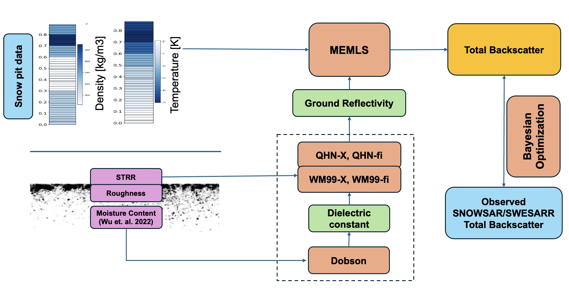
Next, the range for each parameter was used to construct priors for input to the BASE-AM model. Separately, the ground truth snow pit data with imposed nil snow-ground reflectivity were used in MEMLS to estimate the volume backscatter, which was subtracted from the observed total backscatter to infer the contribution of ground backscatter (taken as the “measured” ground backscatter) to be used in the multi-step implementation of BASE-AM as described by [32] as the observed value, accounting for 0.5 dB error for instrument bias. This resulted in a set of parameters for each case of co-located snow pits and SAR pixels. The posterior distribution was then used for quantification of error associated with each parameter and the possible factors contributing to high positive or negative bias relative to the estimates of “measured” ground backscatter were explored. Figure 3 depicts the detailed workflow of the methodology used in this study.
2.3.1. Co-Locating Pits and SAR Measurements
To ensure a precise spatial match among SAR observations and in-situ snow measurements, only the snow pits within the spatial and temporal extent of SAR acquisitions were used. The total observed backscatter at each pit location was then extracted from the co-located SAR pixel as described above. There were no snow pit measurements along the SAR flight lines on the exact day of the flights, and thus snow pit data were surveyed within a few days of the flights assuming that the snowpack does not change significantly in the absence of snowstorms or other precipitation events from one day to another in the winter. Precipitation data from the SNOTEL station at Grand Junction were used to identify the period of time with minimal or no snowfall before and after the SAR flights. Only snow pits excavated during this temporal window and located within the SAR flightlines were considered for analysis to minimize the influence of fresh snow accumulation on backscatter.
Furthermore, since this study focuses on understanding the processes at the snow–ground interface, snow pits within a 90 m radius of forested pixels were excluded to reduce confounding effects from vegetation. Based on these spatial, temporal, and environmental constraints, a total of 32 snow pits met the selection criteria—26 from the 2017 SnowEx campaign and 6 from the 2020 campaign. Stratigraphy data were unavailable for 16 of these pits in 2017. Of these, 6 pits were in spatial proximity to the pits with complete stratigraphic profiles. Based on the assumption that the vertical stratigraphy of snow grain size is spatially homogeneous among nearby pits, the grain size profiles for these 6 pits were reconstructed using data from adjacent sites. This allowed for the consideration of total 22 pits in the final analysis: 16 pits SnowEx’17 pits with co-located VV- and HH-polarized X-band and VV-polarized Ku-band SnowSAR measurements, and 6 pits from SnowEx’20 with co-located VV-polarized X-band SWESARR measurements (Figure 2(b) and 2(c)). Details for all snow pits are provided in Table 2.
2.3.2. Models
- MEMLS3&a snow backscattering model
The radiative transfer model employed in this study to simulate snow-ground backscatter is the Microwave Emission Model for Layered Snowpacks 3 and Active (MEMLS3&a, hereafter MEMLS) based on the improved Born approximation [12,13]. The model assumes a Lambertian distribution for the diffuse part of the bistatic scattering coefficient. MEMLS uses key snowpack properties—including snow depth, SWE, correlation length, temperature, and liquid water content—and sensor parameters (frequency, polarization, incidence angle) to estimate the backscattered signal. The total snow reflectivity computed by passive MEMLS (r) is decomposed into a specular component (rs) and a diffuse component (rd). The specular term is derived from the specular portion of the soil reflectivity, attenuated by snow absorption and scattering effects as the signal propagates through each snow layer (see Eq. 14 in [12]). The diffuse term (rd = r - rs) is then converted into the diffuse component of the backscattering coefficient (σd) using the Lambertian assumption,
where μ0 = cos(θ0) and θ0 is the incidence angle. The specular part of backscatter is calculated using the specular part of reflectivity (rs) (see Eq. 9 in Proksch et al., 2015). Finally, the total backscatter is calculated using:
where Q is the cross-polarization factor. As with most radiative transfer models, MEMLS requires the specification of snow-ground reflectivity as a lower boundary condition, which is calculated using the soil reflectivity models described next.
- b.
- Soil reflectivity models
The soil reflectivity models are used to determine the snow-ground reflectivity based on multiple factors, including the dielectric constant of the soil, which is estimated using the Dobson model [26,27]. Because the frozen soil moisture content required by the Dobson model is difficult to measure and was not available from the SnowEx pits, we used the method of [28] to estimate it for constructing parameter priors. This prior, along with the priors of other parameters, is then used for Bayesian optimization [32,35].
The soil reflectivity models used in this study are Wang and Chaudhary model (1981) also referred to as QHN model [22] and Wëgmuller and Mätzler model (1999) hereafter referred to as WM99 [23]. QHN model is a semi-empirical model that uses roughness height (HR), a polarization mixing parameter (QR), and a parameter accounting for the angular dependency of the reflectivity (NR).
where p is the polarization (can be V or H), , is the H-pol and V-pol reflectivity, , are the V-pol and H-pol Fresnel reflectivity, is the incidence angle and a1, a2, a3, QR, HR, and NR are parameters of the model.
WM99, based on Mo and Schmugge (1987) [24], calculates H-pol reflectivity using soil temperature and soil moisture, and soil roughness, and in a second step, the V-Pol reflectivity is estimated from the modeled H-Pol reflectivity:
where are the parameters, is the wavenumber, is the ground roughness while other notations follow as described for the equation 3.
The calculations in these models as described in Eq. 3 and Eq. 4 include constant parameter values that are critical for the ground reflectivity calculations. Montpetit et al. (2015) [36] tested these models against laboratory experiments for different frequencies and provided a set of parameters that best fit the equations for different frequencies and also a set of frequency-independent parameters (Table 3). They found out that the calibrated WM99 and QHN models yielded similar RMSE, and thus QHN is recommended due to fewer parameters to calibrate. We used the X-band and the frequency-independent parameters of both models to compare them and choose the best-suited model for this study.
- c.
- Bayesian estimation of soil parameters
In a Bayesian retrieval framework, the probability of a geophysical variable x (the posterior distribution) is determined based on prior knowledge of x (the prior distribution), indirect measurements D, and a physical model M(η)— in this case, a snow radiative transfer algorithm — characterized by physical parameters η and statistical error parameters ζ. Given a prior of the parameters P(n) and the likelihood of the observations P(y|n), the posterior probability of the parameters is given by:
In the context of Bayesian inference, the goal is to characterize P(η|y), the posterior probability of physical parameters conditional on measurements informed by the a priori parameter probabilities P(η), which is derived in detail in [34]. This implies maximizing the second term in Eq. 5, the posterior of the backscatter conditional on physical parameters η, which is achieved by evaluating how well model simulations M(η), match the observations y, weighted by the prior knowledge P(η). Building on a Bayesian SWE retrieval framework developed for passive microwave data (Pan et al., 2017 [35]), [37] adapted the approach to active microwave observations. In this approach, snow backscatter is forward-modeled using MEMLS, and unknown geophysical parameters (η) are inferred via Markov Chain Monte Carlo (MCMC) sampling (Metropolis et al., 1953 [38]). The sampler explores the posterior (P(η|y)) by proposing parameter updates and accepting them according to likelihood ratios derived from the mismatch between simulated and observed backscatter, iterating until convergence.
2.4. Quantification of Error
When using a Bayesian retrieval framework, quantifying the uncertainties is a crucial diagnostic step and the primary reason for adopting a probabilistic approach. Unlike deterministic inversion methods that provide single “best-fit” values, Bayesian inference produces full posterior distributions of parameters and simulated backscatter, thereby allowing us to assess the robustness of the retrieval. In this study, where parameters such as surface roughness, volumetric soil moisture, and the specular-to-total reflectivity ratio (STRR) are difficult to measure directly and often vary across scales, rigorous error quantification is essential. Posterior distributions provide insights into both the central tendency of parameter estimates and their spread. Such analysis not only improves confidence in the optimized values but also provides insights into how readily these parameter ranges generalize to other snow-covered regions.
Based on the specified priors and calculated likelihoods during the optimization of observed ground backscatter, the Bayesian framework generates approximately 18,000 posterior samples for each measurement (after discarding burn-in iterations). These samples represent sets of model parameters and the corresponding backscatter estimates, forming the posterior distribution. To quantify error ranges and potential bias in parameter estimation and backscatter calculations, we compute summary statistics including the posterior mean, median, standard deviation, and the 95% highest density interval (HDI).
To assess the reliability of the MCMC sampling, we calculate the Monte Carlo Standard Error (MCSE) and compare it with the posterior standard deviation. For well-converged chains, the MCSE should be substantially smaller than the standard deviation, ensuring that sampling variability does not dominate the posterior uncertainty. Additionally, we compute the split R-hat (Gelman–Rubin statistic), where values close to 1 indicate good mixing and convergence of the chains across independent runs. Together, these diagnostics confirm that the posterior samples provide a robust representation of parameter uncertainties, enabling reliable inference of snow-ground backscatter and associated model parameters.
3. Results
3.1. Soil Reflectivity Model
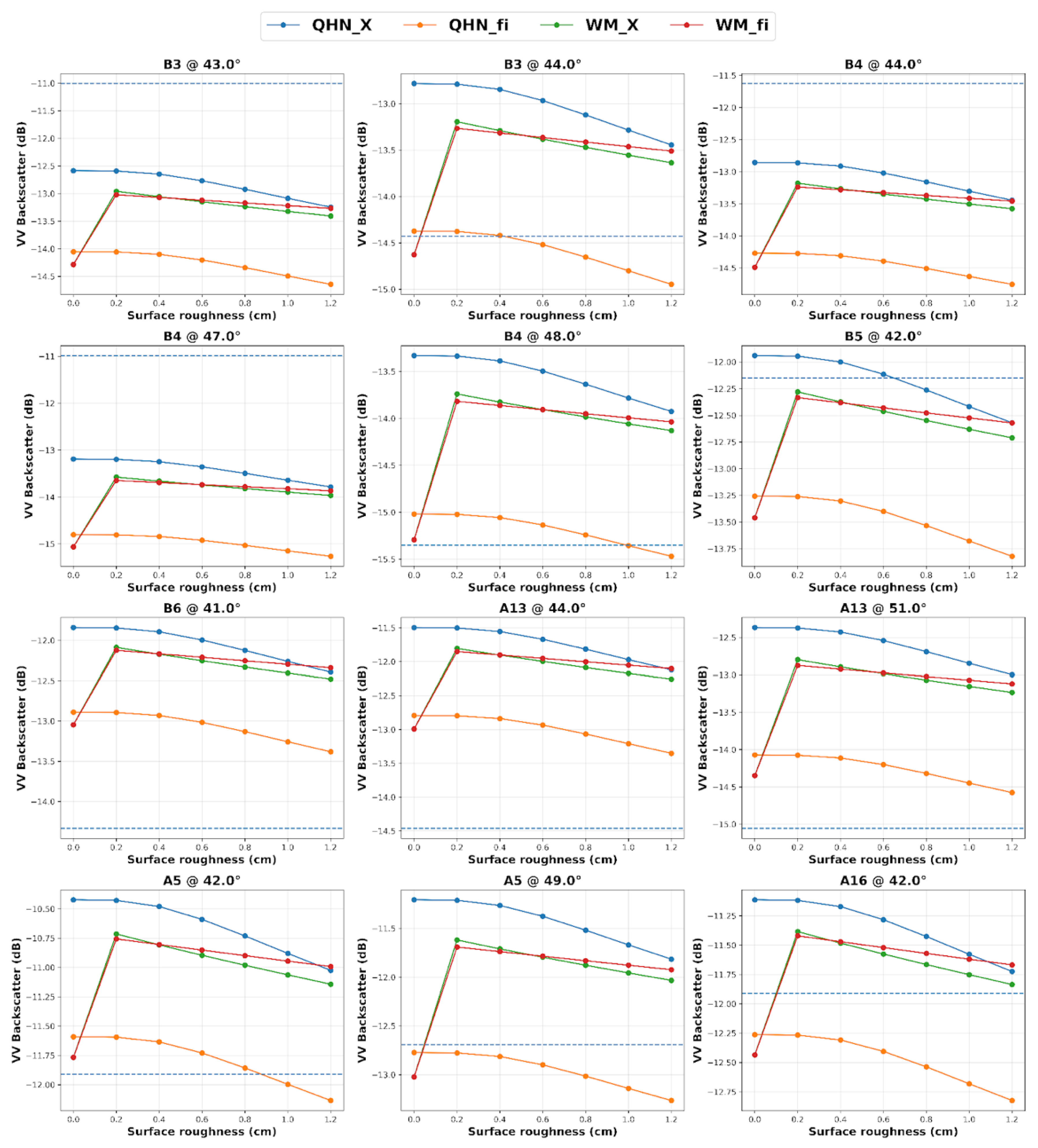
We evaluated backscatter using four soil reflectivity configurations derived from the WM99 and QHN models, each with frequency-independent (fi) and frequency-dependent (X) parameters (Table 3). Among these, the QHN-fi configuration produced the lowest snow-ground reflectivity and consequently the lowest simulated backscatter, followed by WM-X, WM-fi, and QHN-X (Figure A5). The reflectivity given by WM-X and WM-fi are very close, and even the QHN-X reflectivity is close to both.
Figure 4a shows the bias in calculated backscatter averaged for the range of roughness values for each observation. In the preliminary calculations of this study, we can see that we are overestimating for many pits, i.e., there are more pits with positive bias than negative. Since QHN-fi results in lower backscatter as compared to the other three models, and thus smaller bias, it emerges as the best-suited model from parameterizing soil dielectric properties for this study. QHN requires fewer parameters to calibrate [36], and using frequency-independent parameters ensures that the uncertainties associated with the model parameters can be easily utilized in other studies involving multifrequency SAR. Thus, QHN-fi is used for further analysis which is also consistent with [37], who used it with the Dobson model for calculating soil permittivity.
Using the backscatter from QHN-fi as the target variable, we calculated RMSE backscatter over a range of surface roughness values averaged for each pit. Figure 4b shows that the choice of soil model holds RMSE around 1 dB in the final calculation. Note that if in-situ measurements are available, then using QHN-fi as target is not necessary, and the suitability of QHN-fi itself can be assessed.
3.2. SnowSAR Bias Sources - Surficial Melt
Assuming the snowpack to be dry, the model was initialized with zero liquid water content (LWC). However, since the SnowSAR observations are taken in the early afternoon, solar radiation can drive some surficial melting in the snowpack, which can substantially modify the dielectric properties of the top layer of the snowpack [39,40]. Kang and Barros (2012) [11] studied the effect of LWC in the snowpack using passive microwave remote sensing and showed that even small increases in LWC elevate surface reflectivity and alter emissivity. Apart from that, consistent positive biases in Ku-VV (≈5–6 dB across pits) pointed to inadequate representation of near-surface dielectric properties and microphysics, given Ku’s shallower penetration depth and stronger sensitivity to the uppermost layers. To test this hypothesis, the backscatter sensitivity to liquid water content at the top of the snowpack was examined by specifying LWC values in the 0.01-0.06% range in the top 1 cm of the pit snowpacks to emulate surficial melt at mid-day.
Figure 5 shows that the backscatter decreases with increasing LWC, and the magnitude of decrease in the backscatter varied among different pits depending on the microstructure. Volume backscatter from pits with higher correlation length (coarser grains) was less affected by the LWC, while there was a significant decrease in the backscatter with very low correlation length. Moreover, sensitivity to LWC is larger for Ku-band compared to X-band. The X-band backscatter in some pits was not impacted by small amounts of surficial melting up to a certain threshold value, while at Ku-band the backscatter decreases monotonically with LWC. This contrast is consistent with band-dependent scattering mechanisms, with X-band retaining comparatively greater volume-scattering contributions and Ku-band being more dominated by near-surface/surface scattering
To reconcile model and observations, we applied a surficial LWC of 0.0001 to the top 1 cm for all 2017 pits. This successfully corrected the Ku-VV bias while maintaining accurate X-band simulations, accounting for mid-day melt process not captured in the snow pit data.
3.3. Sensitivity Analysis of Ground Parameters
MEMLS with the QHN-fi to estimate the reflectivity at the snow-ground interface was used to estimate the backscatter for both X- and Ku-bands, for each co-located snow pit in 2017 and 2020 (Table 2, Figure 2). For sensitivity analysis, the surface roughness was classified into smooth (0 cm), medium (0.9 cm) and rough (1.2 cm) as in [41]. Due to the low penetration depth, Ku-band backscatter exhibited negligible to very weak sensitivity to ground parameters (Figure 6). In contrast, there is a clear dependence of total backscatter on ground properties at X-band, underscoring the need to characterize these parameters robustly. Specifically, increasing ground surface roughness reduced the simulated backscatter by ~1.5 dB across the tested range, and increasing the STRR produced an additional ~1.0 dB decrease (Figure 7, Figure 8, Figure 9). The estimated backscatter varied for different pits depending on the vertical profile of snowpack. Across sites, simulated backscatter overestimated observations for some pits and underestimated them for most, indicating uncertainty in either the soil-moisture prior or the snowpack characterization. Significant variations in measured backscatter for some pits between near-simultaneous acquisitions suggest other variability sources, including (i) line-of-sight perturbations from nearby vegetation or other land cover (e.g., partial canopy intrusion), (ii) sub-pixel heterogeneity, and (iii) uncertainty in the in-situ snow pit data (disturbance, representativeness, or measurement error), among other factors discussed in this study.
Assuming an instrument error of 0.5 dB for SAR data as in [32], we defined acceptable ground-parameter intervals as those for which the simulated total backscatter lay within ±0.5 dB of the co-located SAR measurement (can be visualized using Figure S1, S2, S3). These intervals were then used as priors in the retrieval algorithm. The volume backscatter of the in-situ snowpack was estimated through forward simulations using MEMLS and subtracted from the total observed backscatter to obtain the “measured” ground backscatter estimate that was used as an observation in the Bayesian optimization algorithm. Observations for which the forward simulation of volume backscatter was greater than the total observed backscatter were eliminated from the study, indicating an error in the observed SAR pixel. For Ku-band, the simulated volume backscatter for all the pits was very close to or greater than the observed total backscatter indicating very low to no contribution of ground backscatter. Moreover, since we had dual polarization HH and VV for 2017 SNOWSAR flights and VV for 2020 SWESARR flights, optimization was conducted for both single pol VV as well as dual pol VV and HH to compare the results.
3.4. Bayesian Parameter Estimation
3.4.1. Dual Polarization
SnowSAR from 2017 had VV and HH polarization acquisitions for X-band; hence, the co-located pits from 2017 were used for dual polarization optimization. The BASE-AM optimization yielded posterior distribution of the parameters and the estimated backscatter that are synthesized in Figure 10. The split Gelman Rubin statistic (R-hat) for these samples was around 1, indicating convergence in the chains (Table A1). Examples of the posterior distribution histogram for each parameter are shown in Figure S7.
The surface roughness varied from smooth (0 cm) to medium (0.9 cm) as classified by [41]. STRR showed the most consistent behavior across all the pits with low variance, a bell-shaped histogram, and a mean of around 65-70%. Soil moisture was the most dominant ground parameter controlling the simulated total backscatter. The soil moisture prior is characterized by high uncertainty. Mechanistically, soil moisture modulates the real part of the soil permittivity (ε) and losses. The retrieved permittivity for most of the pits was between 3.3 to 4 consistent with slightly moist frozen soil, except for some anomalies where the retrieval bias was relatively high in the backscatter. The estimated soil moisture content for some pits (A11, A14, A15, A16) was exceptionally high (~0.095), corresponding to a permittivity of around 4, and for others was low as 0.025 for A7. Analysis of the posterior distribution of backscatter revealed that VV backscatter is in better agreement with the observations than the HH backscatter. Apart from some pits, both VV and HH backscatter posterior mean values are very close to the observed backscatter. The contribution of ground backscatter at X-band is higher for HH than VV polarization. The average bias in the VV backscatter was less than 1 dB for almost all the observations; however, 5 observations showed bias greater than 1 dB, which were analyzed to understand the various sources that can affect the analysis of the snow-ground system using remotely sensed satellite data.
When we separate the observations with bias less than 1 dB, the STRR posterior spans 0.60–0.72 with a mean ≈ 0.65. This narrow dispersion aligns with prior studies that treat STRR as approximately constant (≈0.65–0.70). The sensitivity analysis shows that varying STRR from 0.60 to 0.70 changes the simulated backscatter by only ~0.25 dB, which is well below the adopted SAR radiometric uncertainty (±0.5 dB). Accordingly, fixing STRR = 0.65 is justified and simplifies the inversion without materially affecting fit quality.
3.4.2. Single Polarization
In addition to the snow pits in the previous analysis, the pits and observations from 2020 were also used to optimize the single polarization VV-backscatter (Figure 11). The pits from 2020 showed similar results for STRR, most of them being in the range of 60%-75%, supporting the conclusion that STRR can be held constant around 0.65. Most of the pits had relatively higher soil moisture content, resulting in soil permittivity closer to 4, while a few were relatively drier with soil permittivity around 3.5. The surface roughness for 2020 pits was medium to rough contrasting with smooth values in 2017. For problematic pits (A6, A7, A13) where dual-polarization observations were inconsistent, the single-polarization (VV) inversion reduced bias by 1-2 dB. The adjustment came primarily from surface roughness and STRR, while soil moisture remained stable—a physically plausible result given the soil temperature is very low; the soil is frozen and therefore soil dielectric properties should not change.
For locations where and when the retrievals exhibit large bias, the single-polarization case is more robust because it avoids the “ambiguity” of conflicting HH/VV signals. The results with all the observations can be seen in Figure S8. We then investigated every pit with high bias and examined potential reasons for the error that can be found in the discussion section.
3.5. Error Quantification
In this study, we report the mean, median, standard deviation, 95% highest density interval (HDI) of the posterior chain of each parameter and the corresponding backscatter. Moreover, we investigated the Monte Carlo Standard Error (MCSE), which is very low (<<standard deviation), indicating that it can be ignored (Table A1). The mean and median of STRR were very close, while the posteriors of surface roughness and soil moisture were skewed (Figure S7). Across both single and dual-polarization inversions, the posterior for STRR was highly consistent, with a mean of ~65% and a narrow standard deviation (4-5%). The resulting error in backscatter (~0.125 dB) is well below the instrument uncertainty, strongly validating the use of a fixed STRR value of 0.65 as a robust model simplification.
For surface roughness values, the standard deviation was high. However, it was observed that the smaller the mean surface roughness, i.e., the smoother the surface, the lower is the standard deviation in the posterior distribution. The standard deviation was around 0.2 cm for a mean surface roughness of 0.25 cm, which can lead to an uncertainty of 0.15 dB, and the standard deviation went up to 0.55 cm for surface roughness greater than 1 cm, which can lead to an uncertainty of around 0.3 dB.
The prior of soil moisture was given a range from 0.01 to 0.95, which resulted in a standard deviation of around 0.008 for most of the pits. This change of 0.008 in the soil moisture content can change the real part of the dielectric constant from 3 to 3.16, leading to a change in reflectivity from 0.047 to 0.051. Soil moisture was the most sensitive and least constrained parameter. Consequently, its posterior distribution should be interpreted not as a precise measurement of in-situ moisture, but as an effective parameter that compensates for unmodeled physics and aggregate uncertainties within the snow-soil system to achieve the optimal total backscatter, which is elaborated on in the discussion section.

Table 4.
Mean, Median, 95% HDI, and SD in the posterior distribution of each observation for STRR.
| Pit | Angle (θ0) | STRR mean (%) | Median (%) | HDI_L (%) | HDI_U (%) | SD (%) |
|---|---|---|---|---|---|---|
| B1 | 42.45 | 68.81 | 68.84 | 59.85 | 77.77 | 4.53 |
| B1 | 42.75 | 65.8 | 65.86 | 56.93 | 74.49 | 4.45 |
| B1 | 44.5 | 72.97 | 72.98 | 63.54 | 82.8 | 4.89 |
| B2 | 43.75 | 62.59 | 62.6 | 55.03 | 70.59 | 3.96 |
| B2 | 45.05 | 66.29 | 66.34 | 57.46 | 75.14 | 4.47 |
| B3 | 42.05 | 73.32 | 73.34 | 63.36 | 83.12 | 5.06 |
| B3 | 42.65 | 59.81 | 59.81 | 52.11 | 67.46 | 3.93 |
| B3 | 44.45 | 70.87 | 70.91 | 61.63 | 80.04 | 4.64 |
| B4 | 43.75 | 62.59 | 62.6 | 55.03 | 70.59 | 3.96 |
| B4 | 46.8 | 55.7 | 55.65 | 48.53 | 63.57 | 3.82 |
| B4 | 47.95 | 70.9 | 70.93 | 61.67 | 80.09 | 4.65 |
| B5 | 41.9 | 65.93 | 65.97 | 57.27 | 75.11 | 4.47 |
| A13 | 44 | 73.29 | 73.29 | 63.38 | 83.2 | 5.04 |
| A13 | 51 | 71.09 | 71.14 | 61.53 | 80.49 | 4.75 |
| A5 | 42 | 67.41 | 67.43 | 58.86 | 76.09 | 4.41 |
| A5 | 49 | 66.29 | 66.3 | 57.61 | 75.56 | 4.55 |
| A16 | 42 | 65.96 | 65.97 | 56.86 | 74.61 | 4.49 |
| A16 | 49 | 61.17 | 61.16 | 53.38 | 68.72 | 3.92 |
| A12 | 43 | 70.09 | 70.1 | 60.74 | 79.32 | 4.61 |
| A12 | 49 | 64.48 | 64.55 | 56.18 | 72.54 | 4.16 |
| A11 | 41 | 67.71 | 67.67 | 58.87 | 76.52 | 4.51 |
| A11 | 49 | 61.17 | 61.16 | 53.38 | 68.72 | 3.92 |
| A14 | 42 | 67.41 | 67.43 | 58.86 | 76.09 | 4.41 |
| A14 | 49 | 64.48 | 64.55 | 56.18 | 72.54 | 4.16 |
| A6 | 37 | 64.08 | 64.17 | 55.74 | 72.31 | 4.18 |
| A6 | 48 | 72.19 | 72.23 | 62.82 | 81.42 | 4.7 |
| A7 | 37 | 76.66 | 76.67 | 68.09 | 85.42 | 4.4 |
| A8 | 37 | 64.08 | 64.17 | 55.74 | 72.31 | 4.18 |
| A8 | 48 | 71.14 | 71.28 | 61.7 | 79.89 | 4.64 |
| A9 | 37 | 64.08 | 64.17 | 55.74 | 72.31 | 4.18 |
| A9 | 48 | 65.07 | 65.13 | 56.65 | 73.84 | 4.37 |
| A10 | 37 | 64.08 | 64.17 | 55.74 | 72.31 | 4.18 |
| A10 | 48 | 65.07 | 65.13 | 56.65 | 73.84 | 4.37 |
| A15 | 37 | 64.08 | 64.17 | 55.74 | 72.31 | 4.18 |
| A15 | 48 | 58.37 | 58.34 | 50.99 | 66.13 | 3.86 |
Table 5.
Mean, Median, 95% HDI, and SD in the posterior distribution of each observation for surface roughness (SR).
Table 5.
Mean, Median, 95% HDI, and SD in the posterior distribution of each observation for surface roughness (SR).
| Pit | Angle (θ0) | SR_Mean (cm) | Median (cm) | HDI_L (cm) | HDI_U (cm) | SD (cm) |
|---|---|---|---|---|---|---|
| B1 | 42.45 | 0.69 | 0.72 | 0 | 1.54 | 0.52 |
| B1 | 42.75 | 0.39 | 0.32 | 0 | 1.13 | 0.41 |
| B1 | 44.5 | 1.38 | 1.42 | 0 | 2.18 | 0.53 |
| B2 | 43.75 | 0.23 | 0 | 0 | 0.8 | 0.3 |
| B2 | 45.05 | 0.45 | 0.41 | 0 | 1.23 | 0.44 |
| B3 | 42.05 | 1.36 | 1.4 | 0 | 2.19 | 0.55 |
| B3 | 42.65 | 0.17 | 0 | 0 | 0.68 | 0.25 |
| B3 | 44.45 | 1.06 | 1.13 | 0 | 1.88 | 0.54 |
| B4 | 43.75 | 0.23 | 0 | 0 | 0.8 | 0.3 |
| B4 | 46.8 | 0.12 | 0 | 0 | 0.56 | 0.2 |
| B4 | 47.95 | 1.07 | 1.12 | 0 | 1.9 | 0.56 |
| B5 | 41.9 | 0.4 | 0.34 | 0 | 1.13 | 0.41 |
| A13 | 44 | 1.38 | 1.43 | 0 | 2.19 | 0.53 |
| A13 | 51 | 1.06 | 1.13 | 0 | 1.87 | 0.55 |
| A5 | 42 | 0.52 | 0.52 | 0 | 1.3 | 0.47 |
| A5 | 49 | 0.45 | 0.41 | 0 | 1.23 | 0.44 |
| A16 | 42 | 0.4 | 0.33 | 0 | 1.13 | 0.41 |
| A16 | 49 | 0.21 | 0 | 0 | 0.77 | 0.28 |
| A12 | 43 | 0.9 | 0.96 | 0 | 1.73 | 0.55 |
| A12 | 49 | 0.32 | 0.19 | 0 | 1 | 0.37 |
| A11 | 41 | 0.55 | 0.56 | 0 | 1.35 | 0.48 |
| A11 | 49 | 0.21 | 0 | 0 | 0.77 | 0.28 |
| A14 | 42 | 0.52 | 0.52 | 0 | 1.3 | 0.47 |
| A14 | 49 | 0.32 | 0.19 | 0 | 1 | 0.37 |
| A6 | 37 | 0.25 | 0 | 0 | 0.86 | 0.32 |
| A6 | 48 | 1.23 | 1.26 | 0 | 2.02 | 0.52 |
| A7 | 37 | 1.83 | 1.82 | 1.1 | 2.56 | 0.38 |
| A8 | 37 | 0.25 | 0 | 0 | 0.86 | 0.32 |
| A8 | 48 | 1.04 | 1.1 | 0 | 1.85 | 0.54 |
| A9 | 37 | 0.25 | 0 | 0 | 0.86 | 0.32 |
| A9 | 48 | 0.37 | 0.27 | 0 | 1.09 | 0.4 |
| A10 | 37 | 0.25 | 0 | 0 | 0.86 | 0.32 |
| A10 | 48 | 0.37 | 0.27 | 0 | 1.09 | 0.4 |
| A15 | 37 | 0.25 | 0 | 0 | 0.86 | 0.32 |
| A15 | 48 | 0.15 | 0 | 0 | 0.65 | 0.24 |
Table 6.
Mean, Median, 95% HDI, and SD in the posterior distribution of each observation for soil moisture content.
Table 6.
Mean, Median, 95% HDI, and SD in the posterior distribution of each observation for soil moisture content.
| Pit | Angle (θ0) | Mv_Mean | Median | HDI_L | HDI_U | SD |
|---|---|---|---|---|---|---|
| B1 | 42.45 | 0.064 | 0.064 | 0.046 | 0.082 | 0.009 |
| B1 | 42.75 | 0.084 | 0.084 | 0.069 | 0.095 | 0.009 |
| B1 | 44.5 | 0.038 | 0.038 | 0.02 | 0.053 | 0.01 |
| B2 | 43.75 | 0.093 | 0.095 | 0.081 | 0.095 | 0.005 |
| B2 | 45.05 | 0.08 | 0.079 | 0.065 | 0.095 | 0.01 |
| B3 | 42.05 | 0.031 | 0.031 | 0.02 | 0.048 | 0.01 |
| B3 | 42.65 | 0.094 | 0.095 | 0.087 | 0.095 | 0.003 |
| B3 | 44.45 | 0.054 | 0.053 | 0.037 | 0.072 | 0.009 |
| B4 | 43.75 | 0.093 | 0.095 | 0.081 | 0.095 | 0.005 |
| B4 | 46.8 | 0.095 | 0.095 | 0.093 | 0.095 | 0.001 |
| B4 | 47.95 | 0.053 | 0.053 | 0.036 | 0.071 | 0.009 |
| B5 | 41.9 | 0.082 | 0.081 | 0.066 | 0.095 | 0.01 |
| A13 | 44 | 0.037 | 0.037 | 0.02 | 0.052 | 0.01 |
| A13 | 51 | 0.052 | 0.052 | 0.036 | 0.069 | 0.008 |
| A5 | 42 | 0.071 | 0.071 | 0.057 | 0.095 | 0.009 |
| A5 | 49 | 0.081 | 0.08 | 0.066 | 0.095 | 0.01 |
| A16 | 42 | 0.082 | 0.081 | 0.066 | 0.095 | 0.01 |
| A16 | 49 | 0.094 | 0.095 | 0.086 | 0.095 | 0.003 |
| A12 | 43 | 0.058 | 0.058 | 0.041 | 0.075 | 0.009 |
| A12 | 49 | 0.09 | 0.095 | 0.075 | 0.095 | 0.007 |
| A11 | 41 | 0.069 | 0.069 | 0.051 | 0.088 | 0.009 |
| A11 | 49 | 0.094 | 0.095 | 0.086 | 0.095 | 0.003 |
| A14 | 42 | 0.071 | 0.071 | 0.057 | 0.095 | 0.009 |
| A14 | 49 | 0.09 | 0.095 | 0.075 | 0.095 | 0.007 |
| A6 | 37 | 0.09 | 0.095 | 0.075 | 0.095 | 0.007 |
| A6 | 48 | 0.045 | 0.045 | 0.03 | 0.064 | 0.009 |
| A7 | 37 | 0.021 | 0.02 | 0.02 | 0.029 | 0.003 |
| A8 | 37 | 0.09 | 0.095 | 0.075 | 0.095 | 0.007 |
| A8 | 48 | 0.053 | 0.053 | 0.035 | 0.068 | 0.009 |
| A9 | 37 | 0.09 | 0.095 | 0.075 | 0.095 | 0.007 |
| A9 | 48 | 0.088 | 0.091 | 0.072 | 0.095 | 0.008 |
| A10 | 37 | 0.09 | 0.095 | 0.075 | 0.095 | 0.007 |
| A10 | 48 | 0.088 | 0.091 | 0.072 | 0.095 | 0.008 |
| A15 | 37 | 0.09 | 0.095 | 0.075 | 0.095 | 0.007 |
| A15 | 48 | 0.094 | 0.095 | 0.09 | 0.095 | 0.002 |
Table 7.
Mean, Median, 95% HDI, SD, and bias in the posterior distribution of each observation for VV backscatter.
Table 7.
Mean, Median, 95% HDI, SD, and bias in the posterior distribution of each observation for VV backscatter.
| Pit | Angle (θ0) | VV_Mean | Median | HDI_L | HDI_U | SD | Bias | Obs_VV |
|---|---|---|---|---|---|---|---|---|
| B1 | 42.45 | -16.11 | -16.11 | -16.97 | -15.21 | 0.45 | 0.32 | -16.42 |
| B1 | 42.75 | -14.49 | -14.49 | -15.35 | -13.65 | 0.44 | -0.35 | -14.15 |
| B1 | 44.5 | -19.64 | -19.64 | -20.6 | -18.71 | 0.49 | 1.17 | -20.8 |
| B2 | 43.75 | -13.93 | -13.9 | -14.61 | -13.27 | 0.35 | -0.72 | -13.21 |
| B2 | 45.05 | -15.41 | -15.4 | -16.28 | -14.54 | 0.45 | 0.55 | -15.95 |
| B3 | 42.05 | -19.63 | -19.63 | -20.58 | -18.67 | 0.49 | 0.96 | -20.59 |
| B3 | 42.65 | -13.35 | -13.34 | -13.93 | -12.75 | 0.3 | -0.84 | -12.51 |
| B3 | 44.45 | -17.86 | -17.86 | -18.79 | -16.98 | 0.46 | 0.71 | -18.57 |
| B4 | 43.75 | -13.93 | -13.9 | -14.61 | -13.27 | 0.35 | -0.25 | -13.68 |
| B4 | 46.8 | -14.05 | -14.04 | -14.59 | -13.54 | 0.27 | -1.98 | -12.06 |
| B4 | 47.95 | -18.84 | -18.84 | -19.75 | -17.93 | 0.46 | 0.27 | -19.11 |
| B5 | 41.9 | -14.45 | -14.44 | -15.33 | -13.61 | 0.44 | -0.31 | -14.14 |
| A13 | 44 | -19.62 | -19.62 | -20.6 | -18.71 | 0.49 | 1.22 | -20.84 |
| A13 | 51 | -19.83 | -19.83 | -20.74 | -18.95 | 0.46 | 0.62 | -20.45 |
| A5 | 42 | -15.28 | -15.28 | -16.14 | -14.43 | 0.44 | 0.37 | -15.65 |
| A5 | 49 | -16.42 | -16.42 | -17.29 | -15.5 | 0.45 | -0.09 | -16.33 |
| A16 | 42 | -14.46 | -14.45 | -15.33 | -13.59 | 0.44 | 0.31 | -14.77 |
| A16 | 49 | -15.14 | -15.13 | -15.78 | -14.55 | 0.32 | -0.3 | -14.85 |
| A12 | 43 | -16.95 | -16.94 | -17.86 | -16.06 | 0.46 | 0.87 | -17.82 |
| A12 | 49 | -15.66 | -15.64 | -16.47 | -14.92 | 0.4 | 0.15 | -15.81 |
| A11 | 41 | -15.22 | -15.22 | -16.08 | -14.34 | 0.44 | 0.66 | -15.88 |
| A11 | 49 | -15.14 | -15.13 | -15.78 | -14.55 | 0.32 | -0.7 | -14.44 |
| A14 | 42 | -15.28 | -15.28 | -16.14 | -14.43 | 0.44 | -0.05 | -15.23 |
| A14 | 49 | -15.66 | -15.64 | -16.47 | -14.92 | 0.4 | -0.63 | -15.04 |
| A6 | 37 | -12.73 | -12.71 | -13.51 | -12.01 | 0.39 | 0.22 | -12.95 |
| A6 | 48 | -19.73 | -19.72 | -20.68 | -18.82 | 0.47 | 0.65 | -20.38 |
| A7 | 37 | -20.29 | -20.3 | -21.12 | -19.42 | 0.43 | 0.84 | -21.13 |
| A8 | 37 | -12.73 | -12.71 | -13.51 | -12.01 | 0.39 | -0.09 | -12.64 |
| A8 | 48 | -18.84 | -18.84 | -19.74 | -17.91 | 0.47 | 0.33 | -19.18 |
| A9 | 37 | -12.73 | -12.71 | -13.51 | -12.01 | 0.39 | 0.06 | -12.79 |
| A9 | 48 | -15.58 | -15.56 | -16.39 | -14.74 | 0.42 | 0.3 | -15.87 |
| A10 | 37 | -12.73 | -12.71 | -13.51 | -12.01 | 0.39 | 0.16 | -12.89 |
| A10 | 48 | -15.58 | -15.56 | -16.39 | -14.74 | 0.42 | 0.27 | -15.84 |
| A15 | 37 | -12.73 | -12.71 | -13.51 | -12.01 | 0.39 | -0.08 | -12.65 |
| A15 | 48 | -14.59 | -14.58 | -15.16 | -14.04 | 0.29 | -1.31 | -13.28 |
4. Discussion
This study presents a robust methodology for estimating the snow-ground reflectivity and the parameters involved, however, we assume a simple snow-ground system with no vegetation. Factors such as the forest cover and subgrid scale heterogeneities such as submerged vegetation and landform impact the observed SAR backscatter on the one hand, and measurement errors or insufficient sampling of the in-situ properties of the snowpack at the pits lead to uncertainty in the calculation of snowpack backscatter, as well as the model parameters. Consequently, pits with high bias were examined in detail to get a better understanding of the factors that should be taken care of while performing such a study at the pit scale.
There were cases where the sensitivity analysis revealed abnormally high bias (3-4 dB) for some observations. This was associated with an error in the observation, as SAR data from another flight on the same day had different backscatter for the same location. If the incidence angle is too low or too high, the presence of nearby trees might cause disturbances in the measured backscatter signal, hence hindering the data. Also, the pit data are available at point-scale while the SAR data were aggregated to 30 m from 1 m, thus averaging pixels with forest cover or other types of heterogeneity. Pits A2, A3, A4, being in the proximity of thick forest cover, showed such behavior. Additionally, there was high bias in some of the data points where the pit was located on the edge of the SAR flights such as the case for pit B1 with flight 012, and B2 with flight 005. One of the pits, A1, had very high observed total backscatter as compared to the estimate based on pit data. While analyzing the LULC map, the pit is located very close to a lake that might be a contributing factor, since we averaged the nearby pixels to get a 30 m resolution backscatter.
Some pits even had high bias after the Bayesian optimization, and their detailed analysis revealed some more factors that might be affecting the results. High bias in backscatter observations resulted in extreme soil moisture content estimates (A11, A14, A15, A16, B3, B4 with very high soil moisture and A7 with very low moisture content), and hence the corresponding dielectric constant. The sensitivity of LWC to backscatter for these pits revealed that the pits with excessive soil moisture content, that is the pits with negative bias, are the pits where the backscatter was underestimated and did not need to account for LWC in the snowpack (Figure S5, S6). When a pit is dug for in-situ data collection, there might be small disturbances in the snowpack, leading to characterization errors in the snowpack profile. Pits with low extreme soil moisture corresponding to high bias are the pits that required LWC greater than 0.0001 and hence are compensating with low soil moisture content to reduce the backscatter. Also, presence of even a small layer of light-absorbing particles (LAPs) like dirt that is unreported in the snow pit data and not accounted for in the models can be a contributing factor for it. Therefore, excessive moisture values for frozen soil in the posterior distribution often indicate a model compensating for missed snowpack properties or other errors, rather than reflecting true ground conditions.
Subsurface heterogeneity near pit sites—submerged litter, debris, dense grass, roots— can affect the dielectric constant of the frozen soil, altering backscatter and biasing retrievals. In our dataset, a single SAR snapshot limits our ability to separate these effects from snow/soil state. However, if there are repeated flight overpasses over a region as obtained from an operational satellite mission, then a time series of observations is available that can be used to retrieve the boundary conditions before the accumulation season and improve the determinacy of the snowpack retrieval. In future field campaigns, characterization of soil and physical ground conditions at the pit locations should be considered to provide physical constraints to the boundary condition in the model.
Moreover, in such studies that take place at the pit scale, subscale heterogeneity plays an important role. The observed SAR total backscatter was originally at 1 m resolution, with high variance was reduced by averaging. The SAR backscatter around each pit locations was averaged at different resolutions (1m, 30 m, 60 m, 90 m) to analyze the scaling behavior of the “observed” backscatter as a function of the pixel size that can represent a snow pit. Figure 12a shows that the standard deviation in these values was higher than the 0.5 dB of instrument error considered in Figure 10 and Figure 11. This also explains the high bias in Pit A1, A7. Despite the scatter, there is a trend showing high bias in pits with high standard deviation in the observed backscatter (Figure 12b). Figure S8 shows optimization results for all the pits, except the ones where volume backscatter was lower than the total observed backscatter.
This study demonstrates that the stepwise separation of backscatter at the snow-ground interface from the volume backscatter enables the estimation of realistic bottom boundary conditions to improve the retrieval of snow mass from volume backscatter proposed by [32]. The methodology is general and can be applied anywhere at any time. While it provides valuable insights into the physical parameters governing the snow–ground system, the specific parameters are inherently local to the region of study and different values should be expected elsewhere. Because our primary objective was to examine processes at the snow–ground interface, we employed a simplified system representation that excluded vegetation and forest cover as in [32]. A second limitation concerns scale and representativeness. The scale gap between in-situ pits and SAR pixel resolution emerges as a primary constraint in the evaluation of retrievals. The SAR data at high resolution (1m) have very high variance. This variance decreases with decreased resolution, which in turn increases the scale gap between the snow pit point-scale measurements and the SAR pixel scale backscatter resulting in a loss of heterogeneity, handicapping representativeness.
5. Conclusion
Accurate estimates of snowpack using remote sensing, especially active microwave SAR, have various sources of uncertainty, like the quality of input forcing data, the parameters and constants used in their empirical or semi-empirical equations of both, the PBM and RTM. Here, we focused on understanding and quantifying the error in the boundary conditions of the RTM, i.e., in the estimation of snow-ground backscatter, which serves as a major source of uncertainty. This study used Ku-band VV polarization backscatter to estimate the LWC in the snowpack and X-band VV and HH backscatter to estimate the ground parameters affecting the snow-ground backscatter. Moreover, the QHN model with frequency-independent parameters from [36] was used with the Dobson model to calculate the snow-ground reflectivity. The sensitivity analysis of 2017 Ku-band measurements revealed the presence of surficial melting since the SAR measurements were taken in the early afternoon. Consequently, a LWC of 0.0001 was added to the top 1 cm of the snowpack. Due to shallow penetration, Ku-band is more sensitive to the uppermost layers and surface processes while the ground parameters do not affect the total backscatter. For X-band, the contribution of ground backscatter is higher in HH than VV polarization.
The sources of uncertainty are many including the uncertainty in the snowpack profile, unreported data concerning the presence of dust, depth hoar, or surficial melting, to uncertainty in the SAR data due to subscale heterogeneity or interference from vegetation. The optimized parameters confirmed that the retrieval sensitivity to the specular to total reflectivity ratio (STRR) is minimized in the 0.6-0.7 range and it can be fixed at 0.65. Assuming STRR to be a constant value is also a valid assumption if the study knows the underlying uncertainty associated with it. Irrespective of the observed backscatter in the optimization, STRR did not vary much and was found in 60-70% in the feasible ranges of ground backscatter for X-band. For very low values of ground backscatter, the surface roughness was around 1.2 cm (rough), and it was in the range of 0 cm (smooth) to 0.9 cm (medium) in the feasible range of backscatter. Soil moisture content, the parameter with the most impact on the estimated backscatter, takes a range of values from 2.5% (real part of permittivity = 2.6) if the ground backscatter is around -20 dB to 9.5% (real part of permittivity = 4.05) for ground backscatter around -15 dB. As discussed earlier, this parameter compensates for incomplete information or measurement errors at the snow pits, which in turn impact volume backscatter.
Overall, we demonstrated and independently validated a Bayesian methodology to constrain the critical snow-ground boundary condition in active microwave snow retrievals. By providing a principled way to estimate ground parameter uncertainties, this approach directly supports more efficient and accurate large-scale SWE and SD retrievals from SAR. This study also investigated the uncertainties associated with the parameters that depend upon the value of observed backscatter. Using both – both the VV and HH backscatter and only VV polarization for optimization provided good results with low bias. The pits with high bias were used to explore the factors affecting the accuracy of the forward simulation. Even when using the in-situ snowpack vertical profile, there are some uncertainties related to the characterization of snow layers (example, dry snow, surficial melt, depth hoars, etc.) that can contribute to the bias in the study. This approach’s key strength is its ability to compensate for imperfect snowpack information through parameter estimation, making it robust and practical for real-world applications where model and data uncertainties are unavoidable. Moreover, retrieval of SD and SWE from backscatter using data assimilation [42,43] requires the uncertainties associated with all the parameters, where the uncertainties of ground parameters can be obtained from this methodology.
Optimizing the parameters for 200 X-VV synthetic ground backscatter X-VV values with a fixed 65% STRR and 45 degrees incidence angle revealed that the bias emerges when the observation is too low or too high. Thus, if the SAR measurements display anomalous behavior (too high or too low), the parameters will reflect excessive moisture and surface roughness if we cannot simulate the snowpack accurately. For instance, depth hoar and iced snow will have a very bright observed SAR pixel, while wet snow and LAPs like dust in the snow layer will have relatively darker pixels. If these properties are not accounted for, the parameters attain extreme values to compensate for the lack of information. Table 8 and Figure 13 summarize the response of the BASE-AM model towards various snowpack structure classifications.
Author Contributions
Conceptualization, A.P.B. and A.R.; methodology and validation, A.P.B. and A.R.; formal analysis and investigation, A.R.; resources, A.P.B; data curation, A.R.; writing—original draft preparation, A.R.; writing—review and editing, A.P.B.; visualization, A.R.; supervision, A.P.B. All authors have read and agreed to the published version of the manuscript.
Funding
This research has been supported by the National Aeronautics and Space Administration (grant no. NNX17AL44G to Ana P. Barros) and the National Oceanic and Atmospheric Administration Cooperative Institute for Research to Operations in Hydrology (CIROH) agreement (grant no. NA22NWS4320003 to Ana P. Barros).
Data Availability Statement
The original contributions presented in the study are included in the article, and further inquiries can be directed to the corresponding author.
Acknowledgments
The authors acknowledge NASA’s SnowEx field experiment program and the SnowEx community of investigators that made the data sets used in this work possible. The authors gratefully acknowledge Siddharth Singh and Prabhakar Shrestha for their prior model development and for providing the foundational code used in this study. Finally, the authors are grateful to the anonymous reviewers for their helpful comments and suggestions.
Conflicts of Interest
The contact author has declared that none of the authors has any competing interests.
Abbreviations
The following abbreviations are used in this manuscript:
| RTM | Radiative Transfer Model |
| SAR | Synthetic Aperture Radar |
| STRR | Specular to Total Reflectivity Ratio |
| DEM | Digital Elevation Model |
| LULC | Land Use Land Cover |
| MCMC | Monte Carlo Markov Chain |
Appendix A
Table A1.
Monte Carlo Standard Error (MCSE) and split Gelman Rubic statistic (R-Hat) for each parameter for the MCMC simulations with VV backscatter as observation.
Table A1.
Monte Carlo Standard Error (MCSE) and split Gelman Rubic statistic (R-Hat) for each parameter for the MCMC simulations with VV backscatter as observation.
| Pit | Angle | Soil Moisture (MCSE) |
Soil Moisture (Rhat) | STRR (MCSE) | STRR (Rhat) | Surface Roughness (MCSE) | Surface Roughness (Rhat) | VV Backscatter (MCSE) | VV Backscatter (Rhat) |
|---|---|---|---|---|---|---|---|---|---|
| B1 | 40.25 | 6.00E-05 | 1.00026 | 0.00235 | 1.01104 | 0.00012 | 1.00173 | 0.01006 | 1.00305 |
| B1 | 42.45 | 0.00033 | 1.00179 | 0.00266 | 1.00625 | 0.00013 | 1.00181 | 0.007 | 1.00438 |
| B1 | 42.75 | 0.00029 | 1.00009 | 0.00229 | 1.00449 | 8.00E-05 | 1.0014 | 0.00736 | 1.00132 |
| B1 | 44.5 | 0.00041 | 1.00547 | 0.00302 | 1.01021 | 0.00017 | 1.00154 | 0.00751 | 1.00003 |
| B2 | 39.95 | 0.00042 | 1.00152 | 0.00301 | 1.00886 | 0.00018 | 0.99995 | 0.00767 | 1.00044 |
| B2 | 43.75 | 9.00E-05 | 0.99998 | 0.0019 | 1.00956 | 5.00E-05 | 0.99995 | 0.0096 | 1.00591 |
| B2 | 45.05 | 0.00035 | 0.99995 | 0.0025 | 1.00624 | 9.00E-05 | 1.00022 | 0.00647 | 1.00217 |
| A1 | 32 | 0 | 1.00004 | 0.00187 | 1.00702 | 1.00E-05 | 1.00007 | 0.01 | 1.00696 |
| A1 | 54 | 3.00E-05 | 1.00012 | 0.00195 | 1.00801 | 4.00E-05 | 0.99995 | 0.01247 | 1.00698 |
| B3 | 42.05 | 0.00046 | 1.00512 | 0.00321 | 1.01218 | 0.00018 | 1.00017 | 0.00824 | 0.99995 |
| B3 | 42.65 | 4.00E-05 | 0.99998 | 0.00192 | 1.00801 | 4.00E-05 | 0.99997 | 0.01174 | 1.00631 |
| B3 | 44.45 | 0.00038 | 1.00121 | 0.00263 | 1.00872 | 0.00016 | 0.99997 | 0.00644 | 1.00059 |
| B4 | 43.75 | 9.00E-05 | 0.99998 | 0.0019 | 1.00956 | 5.00E-05 | 0.99995 | 0.0096 | 1.00591 |
| B4 | 46.8 | 2.00E-05 | 1.00013 | 0.00189 | 1.01086 | 3.00E-05 | 0.99999 | 0.01206 | 1.00957 |
| B4 | 47.95 | 0.00033 | 0.99998 | 0.00268 | 1.0085 | 0.00016 | 1.00153 | 0.00628 | 1.00186 |
| B5 | 41.9 | 0.00031 | 0.99995 | 0.00243 | 1.00282 | 8.00E-05 | 1.00027 | 0.0065 | 1.00094 |
| A13 | 44 | 0.00057 | 1.00167 | 0.00327 | 1.01397 | 0.00016 | 1.00024 | 0.00857 | 1.00036 |
| A13 | 51 | 0.00033 | 1.00039 | 0.00281 | 1.01232 | 0.00015 | 1.00079 | 0.00643 | 1.00073 |
| A5 | 42 | 0.00033 | 1.00029 | 0.00233 | 1.01348 | 0.00011 | 1.0009 | 0.00746 | 1.00178 |
| A5 | 49 | 0.00034 | 1.00003 | 0.00254 | 1.01057 | 9.00E-05 | 1.00092 | 0.00673 | 1.00169 |
| A16 | 42 | 0.00034 | 1.00004 | 0.0025 | 1.00345 | 8.00E-05 | 1.00016 | 0.00642 | 1.00052 |
| A16 | 49 | 6.00E-05 | 0.99995 | 0.00192 | 1.00722 | 5.00E-05 | 0.99995 | 0.01122 | 1.0048 |
| A12 | 43 | 0.00034 | 1.00002 | 0.00266 | 1.00781 | 0.00016 | 1.00179 | 0.0063 | 1.00119 |
| A12 | 49 | 0.00017 | 0.99999 | 0.00214 | 1.00868 | 6.00E-05 | 1.00042 | 0.00819 | 1.00242 |
| A11 | 41 | 0.00033 | 1.00011 | 0.0026 | 1.01033 | 0.00011 | 1.00046 | 0.00698 | 1.00194 |
| A11 | 49 | 6.00E-05 | 0.99995 | 0.00192 | 1.00722 | 5.00E-05 | 0.99995 | 0.01122 | 1.0048 |
| A14 | 42 | 0.00033 | 1.00029 | 0.00233 | 1.01348 | 0.00011 | 1.0009 | 0.00746 | 1.00178 |
| A14 | 49 | 0.00017 | 0.99999 | 0.00214 | 1.00868 | 6.00E-05 | 1.00042 | 0.00819 | 1.00242 |
| A6 | 37 | 0.00016 | 1.00001 | 0.00215 | 1.0094 | 6.00E-05 | 1.00032 | 0.00868 | 1.00343 |
| A6 | 48 | 0.00033 | 1.00085 | 0.00272 | 1.00078 | 0.00015 | 1.00061 | 0.00641 | 1.00117 |
| A7 | 37 | 8.00E-05 | 1.00075 | 0.0024 | 1.00759 | 0.00011 | 1.00056 | 0.00969 | 1.00168 |
| A8 | 37 | 0.00016 | 1.00001 | 0.00215 | 1.0094 | 6.00E-05 | 1.00032 | 0.00868 | 1.00343 |
| A8 | 48 | 0.00035 | 0.99996 | 0.00265 | 1.00425 | 0.00016 | 1.00015 | 0.0065 | 1.00074 |
| A9 | 37 | 0.00016 | 1.00001 | 0.00215 | 1.0094 | 6.00E-05 | 1.00032 | 0.00868 | 1.00343 |
| A9 | 48 | 0.00024 | 1.0001 | 0.00229 | 1.00639 | 7.00E-05 | 1.00013 | 0.00748 | 1.00165 |
| A10 | 37 | 0.00016 | 1.00001 | 0.00215 | 1.0094 | 6.00E-05 | 1.00032 | 0.00868 | 1.00343 |
| A10 | 48 | 0.00024 | 1.0001 | 0.00229 | 1.00639 | 7.00E-05 | 1.00013 | 0.00748 | 1.00165 |
| A15 | 37 | 0.00016 | 1.00001 | 0.00215 | 1.0094 | 6.00E-05 | 1.00032 | 0.00868 | 1.00343 |
| A15 | 48 | 3.00E-05 | 1.00019 | 0.00185 | 1.00859 | 4.00E-05 | 0.99996 | 0.01184 | 1.00769 |
Table A2.
All the observations from the co-located pits that were used in the study.
| NSDIC Pit name | Pit Name (used in the study) | Latitude | Longitude | Date | Incidence Angle (θ0) |
Realization |
|---|---|---|---|---|---|---|
| 28S | A1 | 39.0122478 | -108.1379938 | 2017-02-25 | 32 | 1 |
| 54 | 2 | |||||
| 78N | A2 | 39.04342878 | -107.9202531 | 2017-02-25 | 31 | 1 |
| 40 | 2 | |||||
| 92E | A3 | 39.0510518 | -107.885109 | 2017-02-22 | 41 | 1 |
| 48 | 2 | |||||
| 92W | A4 | 39.0510159 | -107.8876494 | 2017-02-22 | 42 | 1 |
| 49 | 2 | |||||
| KC1C | A5 | 39.01363394 | -108.1838735 | 2017-02-20 | 42 | 1 |
| 49 | 2 | |||||
| MTR4_0000 | A6 | 39.0300503 | -108.0331353 | 2017-02-24 | 37 | 1 |
| 48 | 2 | |||||
| MTR4_0800 | A7 | 39.03005659 | -108.0332395 | 2017-02-24 | 37 | 1 |
| 48 | 2 | |||||
| MTR4_1390 | A8 | 39.03005509 | -108.0332972 | 2017-02-24 | 37 | 1 |
| 48 | 2 | |||||
| MTR4_2000 | A9 | 39.03005329 | -108.0333664 | 2017-02-24 | 37 | 1 |
| 48 | 2 | |||||
| MTR4_2500 | A10 | 39.03005179 | -108.0334241 | 2017-02-24 | 48 | 1 |
| 37 | 2 | |||||
| KC1S* | A11 | 39.01344468 | -108.1838766 | 2017-02-20 | 41 | 1 |
| 49 | 2 | |||||
| KC1N* | A12 | 39.01381389 | -108.1838816 | 2017-02-20 | 43 | 1 |
| 49 | 2 | |||||
| 67N* | A13 | 39.03245119 | -108.0291492 | 2017-02-22 | 44 | 1 |
| 51 | 2 | |||||
| KC1W* | A14 | 39.01362669 | -108.1841388 | 2017-02-20 | 42 | 1 |
| 49 | 2 | |||||
| MTR4_4500* | A15 | 39.03005478 | -108.0336552 | 2017-02-24 | 37 | 1 |
| 48 | 2 | |||||
| KC1E* | A16 | 39.01363219 | -108.1836079 | 2017-02-20 | 42 | 1 |
| 49 | 2 | |||||
| 1S1 | B1 | 39.02119889 | -108.20559 | 2020-01-29 | 42.45 | 1 |
| 40.25 | 2 | |||||
| 44.5 | 3 | |||||
| 42.75 | 4 | |||||
| 41.5 | 5 | |||||
| 1S2 | B2 | 39.019948 | -108.203396 | 2020-02-08 | 39.95 | 1 |
| 44.55 | 2 | |||||
| 42.95 | 3 | |||||
| 46.9 | 4 | |||||
| 45.05 | 5 | |||||
| 43.75 | 6 | |||||
| 2S3 | B3 | 39.021089 | -108.202889 | 2020-01-29 | 42.05 | 1 |
| 44.45 | 2 | |||||
| 42.65 | 3 | |||||
| 41.35 | 4 | |||||
| 2S4 | B4 | 39.017951 | -108.201292 | 2020-02-05 | 43.75 | 1 |
| 47.95 | 2 | |||||
| 46.8 | 3 | |||||
| 2S7 | B5 | 39.01866002 | -108.197788 | 2020-02-08 | 41.9 | 1 |
| 3S5 | B6 | 39.01911256 | -108.1986242 | 2020-01-29 | 41.15 | 2 |
Figure A1.
Sensitivity Analysis of Ku-band VV backscatter for a range of surface roughness and STRR for 2017 observations.
Figure A1.
Sensitivity Analysis of Ku-band VV backscatter for a range of surface roughness and STRR for 2017 observations.
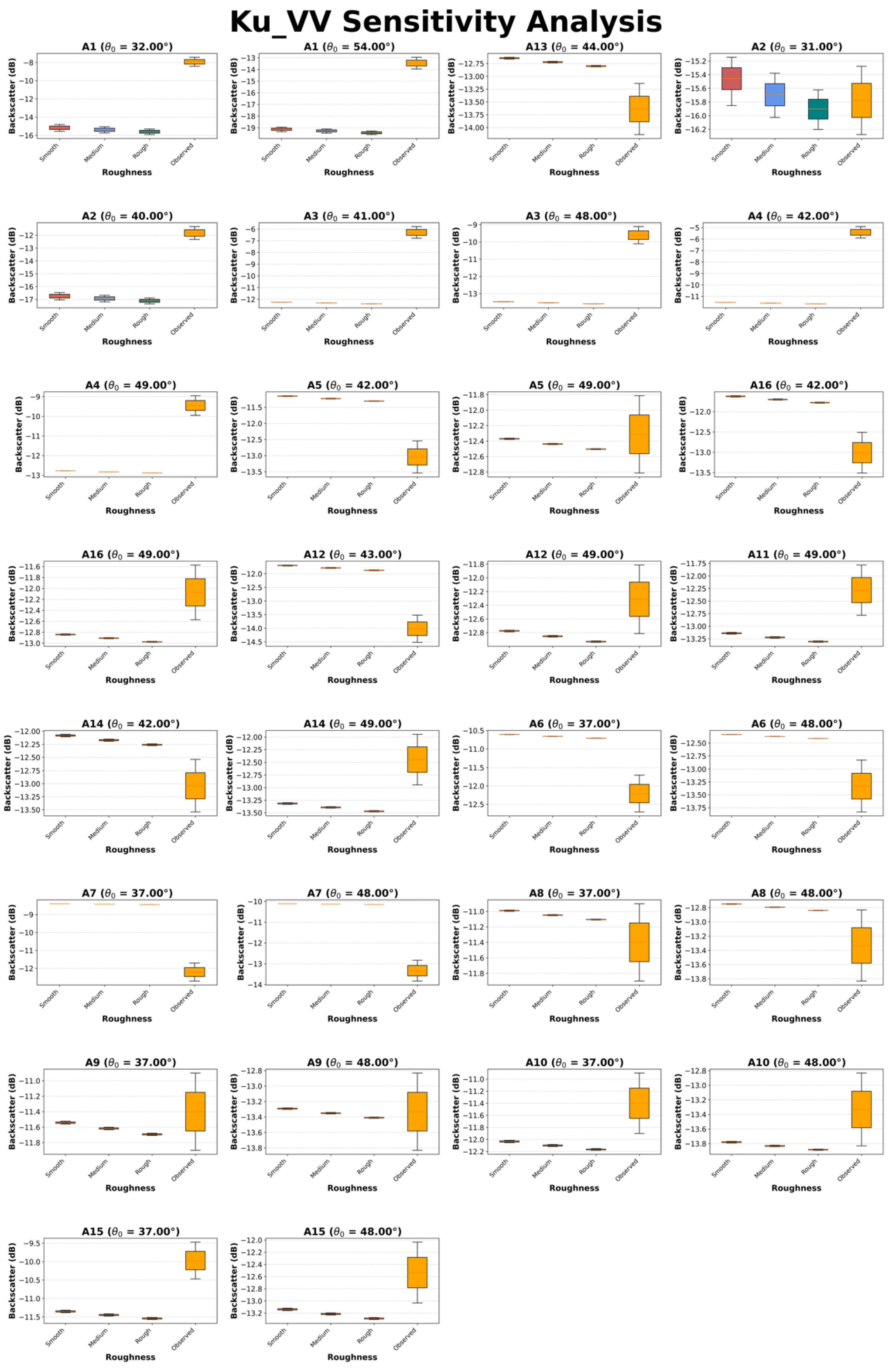
Figure A2.
Sensitivity Analysis of X-band HH backscatter for a range of surface roughness and STRR for 2017 observations.
Figure A2.
Sensitivity Analysis of X-band HH backscatter for a range of surface roughness and STRR for 2017 observations.
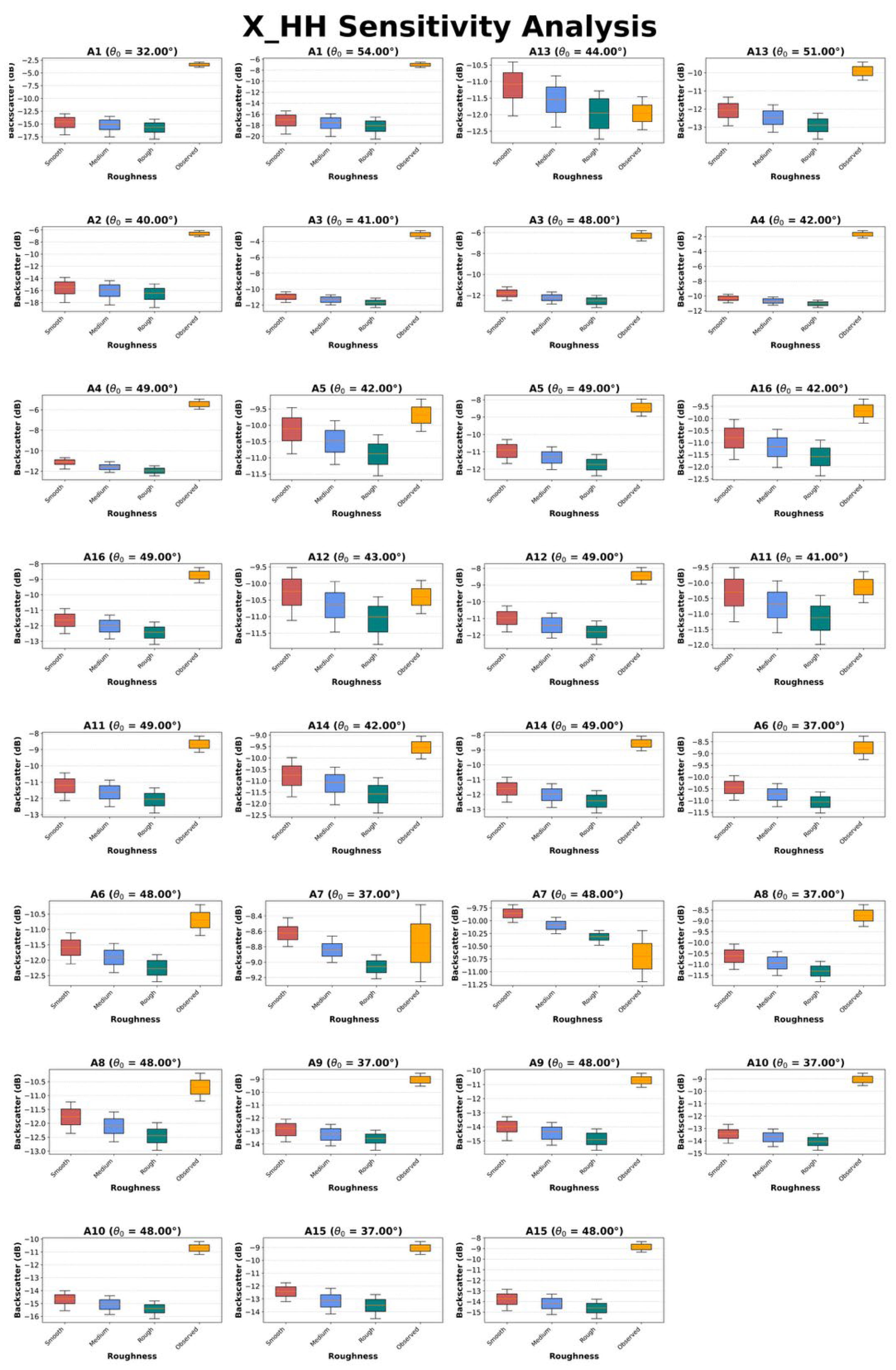
Figure A3.
Sensitivity Analysis of X-band VV backscatter for a range of surface roughness and STRR for all the observations – 2017.
Figure A3.
Sensitivity Analysis of X-band VV backscatter for a range of surface roughness and STRR for all the observations – 2017.
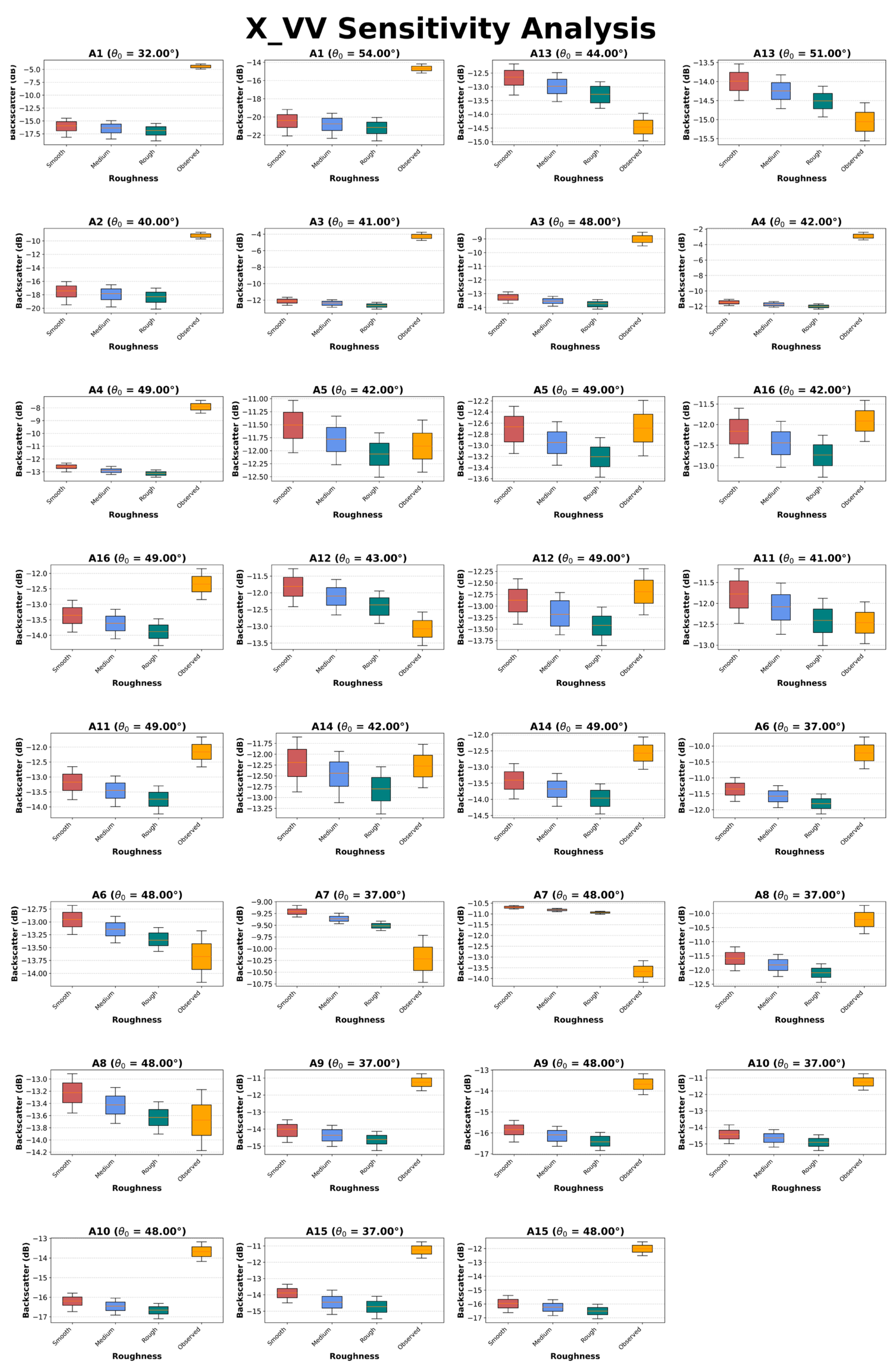
Figure A4.
Sensitivity Analysis of X-band VV backscatter for a range of surface roughness and STRR for all the observations – 2020.
Figure A4.
Sensitivity Analysis of X-band VV backscatter for a range of surface roughness and STRR for all the observations – 2020.
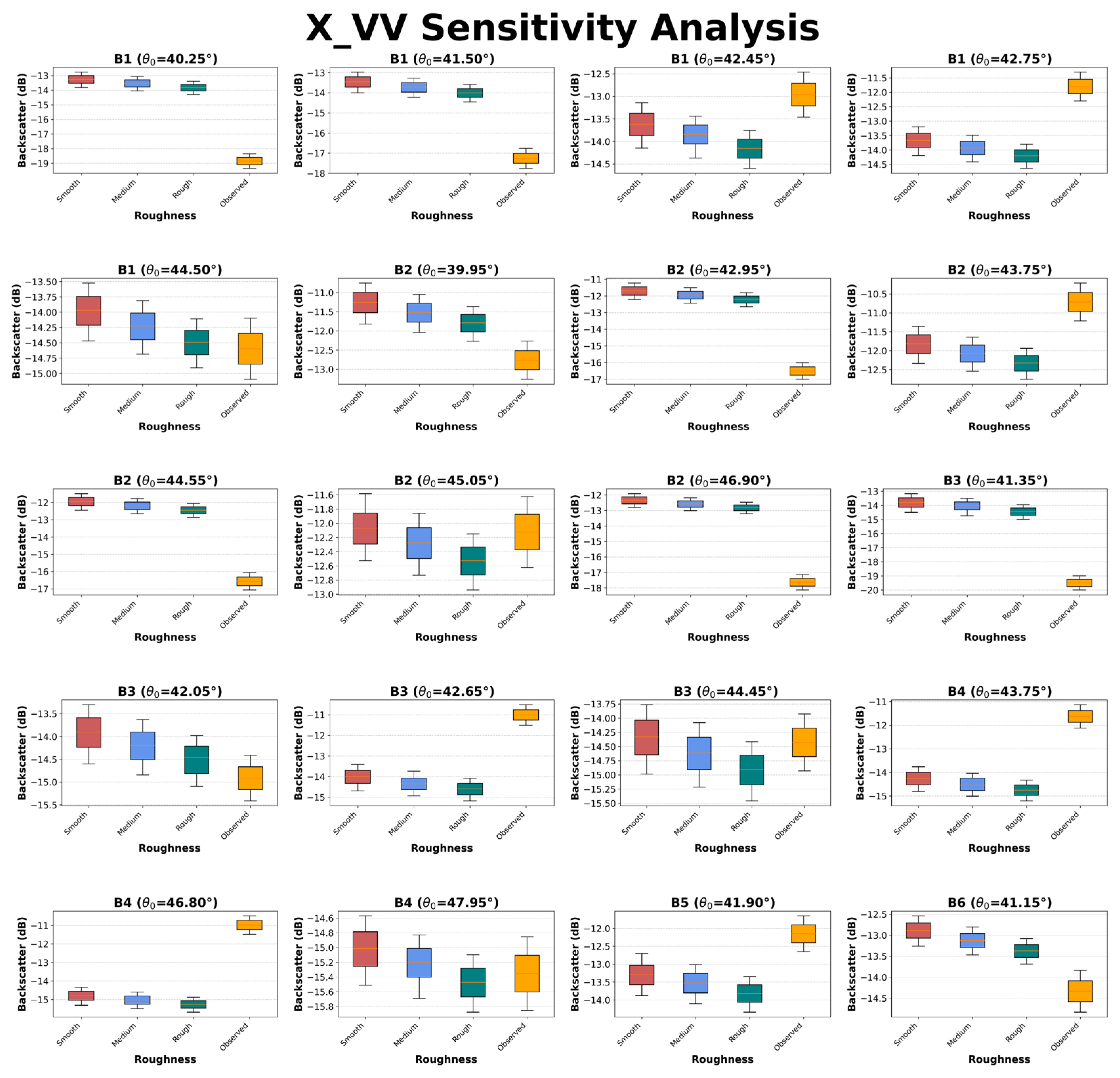
Figure A5.
Simulated backscatter using the four soil models for STRR = 65% and for a range of surface roughness values shown for a few pits.
Figure A5.
Simulated backscatter using the four soil models for STRR = 65% and for a range of surface roughness values shown for a few pits.
References
- Barnett, T.P.; Adam, J.C.; Lettenmaier, D.P. Potential impacts of a warming climate on water availability in snow-dominated regions. Nature 2005, 438, 303–309. [Google Scholar] [CrossRef] [PubMed]
- Sturm, M.; Goldstein, M.A.; Parr, C. Water and life from snow: A trillion dollar science question. Water Resour. Res. 2017, 53, 3534–3544. [Google Scholar] [CrossRef]
- Pulliainen, J. Retrieval of Regional Snow Water Equivalent from Space-Borne Passive Microwave Observations. Remote. Sens. Environ. 2001, 75, 76–85. [Google Scholar] [CrossRef]
- Derksen, C.; Walker, A.; Goodison, B. A comparison of 18 winter seasons of in situ and passive microwave-derived snow water equivalent estimates in Western Canada. Remote. Sens. Environ. 2003, 88, 271–282. [Google Scholar] [CrossRef]
- Moser, C.L.; Aziz, O.; Tootle, G.A.; Lakshmi, V.; Kerr, G. A comparison of SNOTEL and AMSR-E snow water equivalent datasets in western U.S. watersheds. In Proceedings of the Third International Workshop on Knowledge Discovery from Sensor Data; Association for Computing Machinery: New York, NY, USA, 2009; pp. 32–38. [Google Scholar]
- Dickinson, R.E. Land Surface Processes and Climate—Surface Albedos and Energy Balance. In Advances in Geophysics; Elsevier: Amsterdam, The Netherlands, 1983; Volume 25, pp. 305–353. [Google Scholar]
- Kumar, S.; Mocko, D.; Vuyovich, C.; Peters-Lidard, C. Impact of Surface Albedo Assimilation on Snow Estimation. Remote. Sens. 2020, 12, 645. [Google Scholar] [CrossRef]
- Bormann, K.J.; Brown, R.D.; Derksen, C.; Painter, T.H. Estimating snow-cover trends from space. Nat. Clim. Chang. 2018, 8, 924–928. [Google Scholar] [CrossRef]
- Che, T.; Li, X.; Jin, R.; Huang, C. Assimilating passive microwave remote sensing data into a land surface model to improve the estimation of snow depth. Remote. Sens. Environ. 2014, 143, 54–63. [Google Scholar] [CrossRef]
- Pan, J. Application of Passive and Active Microwave Remote Sensing for Snow Water Equivalent Estimation. The Ohio State University, 2017. Available online: https://etd.ohiolink.edu/acprod/odb_etd/etd/r/1501/10?clear=10&p10_accession_num=osu149737615724025.
- Kang, D.H.; Barros, A.P.; Dery, S.J. Evaluating Passive Microwave Radiometry for the Dynamical Transition From Dry to Wet Snowpacks. IEEE Trans. Geosci. Remote. Sens. 2013, 52, 3–15. [Google Scholar] [CrossRef]
- Proksch, M.; Mätzler, C.; Wiesmann, A.; Lemmetyinen, J.; Schwank, M.; Löwe, H.; Schneebeli, M. MEMLS3&a: Microwave Emission Model of Layered Snowpacks adapted to include backscattering. Geosci. Model Dev. 2015, 8, 2611–2626. [Google Scholar] [CrossRef]
- Wiesmann, A.; Mätzler, C. Microwave Emission Model of Layered Snowpacks. Remote. Sens. Environ. 1999, 70, 307–316. [Google Scholar] [CrossRef]
- Tsang, L.; Pan, J.; Liang, D.; Li, Z.; Cline, D.W.; Tan, Y. Modeling Active Microwave Remote Sensing of Snow Using Dense Media Radiative Transfer (DMRT) Theory With Multiple-Scattering Effects. IEEE Trans. Geosci. Remote. Sens. 2007, 45, 990–1004. [Google Scholar] [CrossRef]
- Picard, G.; Sandells, M.; Löwe, H. SMRT: an active–passive microwave radiative transfer model for snow with multiple microstructure and scattering formulations (v1.0). Geosci. Model Dev. 2018, 11, 2763–2788. [Google Scholar] [CrossRef]
- Kang, D.H.; Barros, A.P. Observing System Simulation of Snow Microwave Emissions Over Data Sparse Regions— Part I: Single Layer Physics. IEEE Trans. Geosci. Remote. Sens. 2011, 50, 1785–1805. [Google Scholar] [CrossRef]
- Kang, D.H.; Barros, A.P. Observing System Simulation of Snow Microwave Emissions Over Data Sparse Regions—Part II: Multilayer Physics. IEEE Trans. Geosci. Remote. Sens. 2011, 50, 1806–1820. [Google Scholar] [CrossRef]
- Bartelt, P.; Lehning, M. A physical SNOWPACK model for the Swiss avalanche warning. Cold Reg. Sci. Technol. 2002, 35, 123–145. [Google Scholar] [CrossRef]
- Brun, E.; Martin, Ε.; Simon, V.; Gendre, C.; Coleou, C. An Energy and Mass Model of Snow Cover Suitable for Operational Avalanche Forecasting. J. Glaciol. 1989, 35, 333–342. [Google Scholar] [CrossRef]
- U. F., T. Microwave Remote Sensing. Active and Passive 1986, vol. 0, p. Chap. 7. [Google Scholar]
- Singh, V. P.; Singh, P.; Haritashya, U. K. Encyclopedia of Snow, Ice and Glaciers; Springer Science & Business Media, 2011. [Google Scholar]
- Wang, J.R.; Choudhury, B.J. Remote sensing of soil moisture content, over bare field at 1.4 GHz frequency. J. Geophys. Res. Oceans 1981, 86, 5277–5282. [Google Scholar] [CrossRef]
- Wegmuller, U.; Matzler, C. Rough bare soil reflectivity model. IEEE Trans. Geosci. Remote. Sens. 1999, 37, 1391–1395. [Google Scholar] [CrossRef]
- Mo, T.; Schmugge, T.J. A Parameterization of the Effect of Surface Roughness on Microwave Emission. IEEE Trans. Geosci. Remote. Sens. 1987, GE-25, 481–486. [Google Scholar] [CrossRef]
- Tan, Y.; Li, Z.; Tse, K.K.; Tsang, L. Microwave model of remote sensing of snow based on dense media radiative transfer theory with numerical Maxwell model of 3D simulations (NMM3D). Proceedings. 2005 IEEE International Geoscience and Remote Sensing Symposium, 2005. IGARSS ’05, July 2005; pp. 578–581. [Google Scholar] [CrossRef]
- Dobson, M.C.; Ulaby, F.T.; Hallikainen, M.T.; El-Rayes, M.A. Microwave Dielectric Behavior of Wet Soil-Part II: Dielectric Mixing Models. IEEE Trans. Geosci. Remote Sens. 1985, 23, 35–46. [Google Scholar] [CrossRef]
- Hallikainen, M.T.; Ulaby, F.T.; Dobson, M.C.; El-Rayes, M.A.; Wu, L.-K. Microwave Dielectric Behavior of Wet Soil-Part 1: Empirical Models and Experimental Observations. IEEE Trans. Geosci. Remote. Sens. 1985, GE-23, 25–34. [Google Scholar] [CrossRef]
- Wu, S.; Zhao, T.; Pan, J.; Xue, H.; Zhao, L.; Shi, J. Improvement in Modeling Soil Dielectric Properties During Freeze-Thaw Transitions. IEEE Geosci. Remote. Sens. Lett. 2022, 19, 1–5. [Google Scholar] [CrossRef]
- King, J.; Derksen, C.; Toose, P.; Langlois, A.; Larsen, C.; Lemmetyinen, J.; Marsh, P.; Montpetit, B.; Roy, A.; Rutter, N.; et al. The influence of snow microstructure on dual-frequency radar measurements in a tundra environment. Remote. Sens. Environ. 2018, 215, 242–254. [Google Scholar] [CrossRef]
- Lemmetyinen, J.; Derksen, C.; Rott, H.; Macelloni, G.; King, J.; Schneebeli, M.; Wiesmann, A.; Leppänen, L.; Kontu, A.; Pulliainen, J. Retrieval of Effective Correlation Length and Snow Water Equivalent from Radar and Passive Microwave Measurements. Remote. Sens. 2018, 10, 170. [Google Scholar] [CrossRef]
- Zhu, J.; Tan, S.; Tsang, L.; Kang, D.; Kim, E. Snow Water Equivalent Retrieval Using Active and Passive Microwave Observations. Water Resour. Res. 2021, 57. [Google Scholar] [CrossRef]
- Singh, S.; Durand, M.; Kim, E.; Barros, A.P. Bayesian physical–statistical retrieval of snow water equivalent and snow depth from X- and Ku-band synthetic aperture radar – demonstration using airborne SnowSAr in SnowEx'17. Cryosphere 2024, 18, 747–773. [Google Scholar] [CrossRef]
- Elder, K.; Brucker, L.; Hiemstra, C.; Marshall, H.-P. “SnowEx17 Community Snow Pit Measurements, Version 1,” NASA National Snow and Ice Data Center Distributed Active Archive Center (DAAC) data set, p. Q0310G1XULZS. 2018. [Google Scholar] [CrossRef]
- Mason, M.; Marshall, H.-P.; McCormick, M.; Craaybeek, D.; Elder, K.; Vuyovich, C. “SnowEx20 Time Series Snow Pit Measurements, Version 1,” NASA National Snow and Ice Data Center Distributed Active Archive Center (DAAC) data set, p. POT9E0FFUUD1; Jan 2023. [Google Scholar] [CrossRef]
- Pan, J.; Durand, M.T.; Jagt, B.J.V.; Liu, D. Application of a Markov Chain Monte Carlo algorithm for snow water equivalent retrieval from passive microwave measurements. Remote. Sens. Environ. 2017, 192, 150–165. [Google Scholar] [CrossRef]
- Montpetit, B.; Royer, A.; Wigneron, J.-P.; Chanzy, A.; Mialon, A. Evaluation of multi-frequency bare soil microwave reflectivity models. Remote. Sens. Environ. 2015, 162, 186–195. [Google Scholar] [CrossRef]
- Pan, J.; Durand, M.; Lemmetyinen, J.; Liu, D.; Shi, J. Snow water equivalent retrieved from X- and dual Ku-band scatterometer measurements at Sodankylä using the Markov Chain Monte Carlo method. Cryosphere 2024, 18, 1561–1578. [Google Scholar] [CrossRef]
- Metropolis, N.; Rosenbluth, A.W.; Rosenbluth, M.N.; Teller, A.H.; Teller, E. Equation of state calculations by fast computing machines. J. Chem. Phys. 1953, 21, 1087–1092. [Google Scholar] [CrossRef]
- Ulaby, F.T.; Stiles, W.H. Microwave response of snow. Adv. Space Res. 1981, 1, 131–149. [Google Scholar] [CrossRef]
- Cao, Y.; Barros, A.P. Weather-Dependent Nonlinear Microwave Behavior of Seasonal High-Elevation Snowpacks. Remote. Sens. 2020, 12, 3422. [Google Scholar] [CrossRef]
- Choudhury, B.J.; Schmugge, T.J.; Chang, A.; Newton, R.W. Effect of surface roughness on the microwave emission from soils. J. Geophys. Res. Oceans 1979, 84, 5699–5706. [Google Scholar] [CrossRef]
- Shrestha, P.; Barros, A.P. Multi-Physics Data Assimilation Framework for Remotely Sensed Snowpacks to Improve Water Prediction. Water Resour. Res. 2025, 61. [Google Scholar] [CrossRef]
- Shrestha, P.; Barros, A.P. Assimilation of L-band interferometric synthetic aperture radar (InSAR) snow depth retrievals for improved snowpack quantification. Cryosphere 2025, 19, 2895–2911. [Google Scholar] [CrossRef]
Figure 1.
(a) LULC (top right) and (b) DEM (bottom right) of the study site, Grand Mesa, CO.
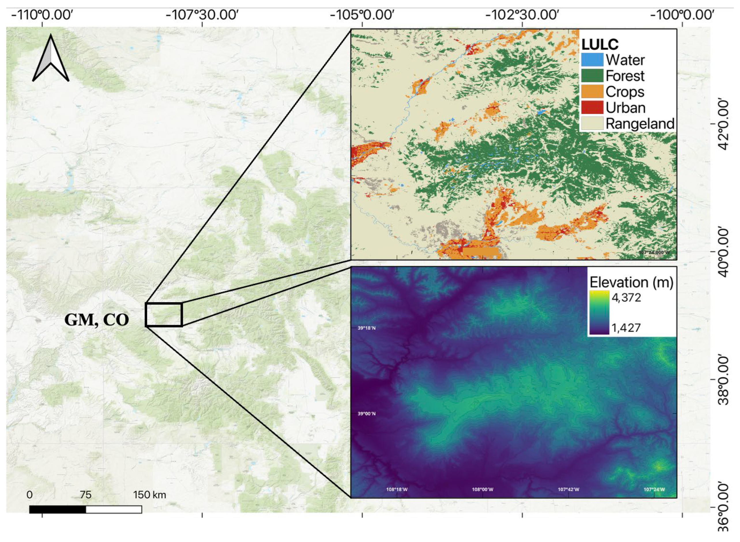
Figure 2.
(a) Snow pits in the Snow Ex ‘17 dataset (red) and Snow Ex ‘20 dataset (pink) laid over DEM of the study site along with the flight paths of SnowSAR (bigger black boxes) and SWESARR (smaller yellow boxes on the left); (b) Co-located pits used for this study in 2017; and (c) Co-located pits were used for this study in 2020.
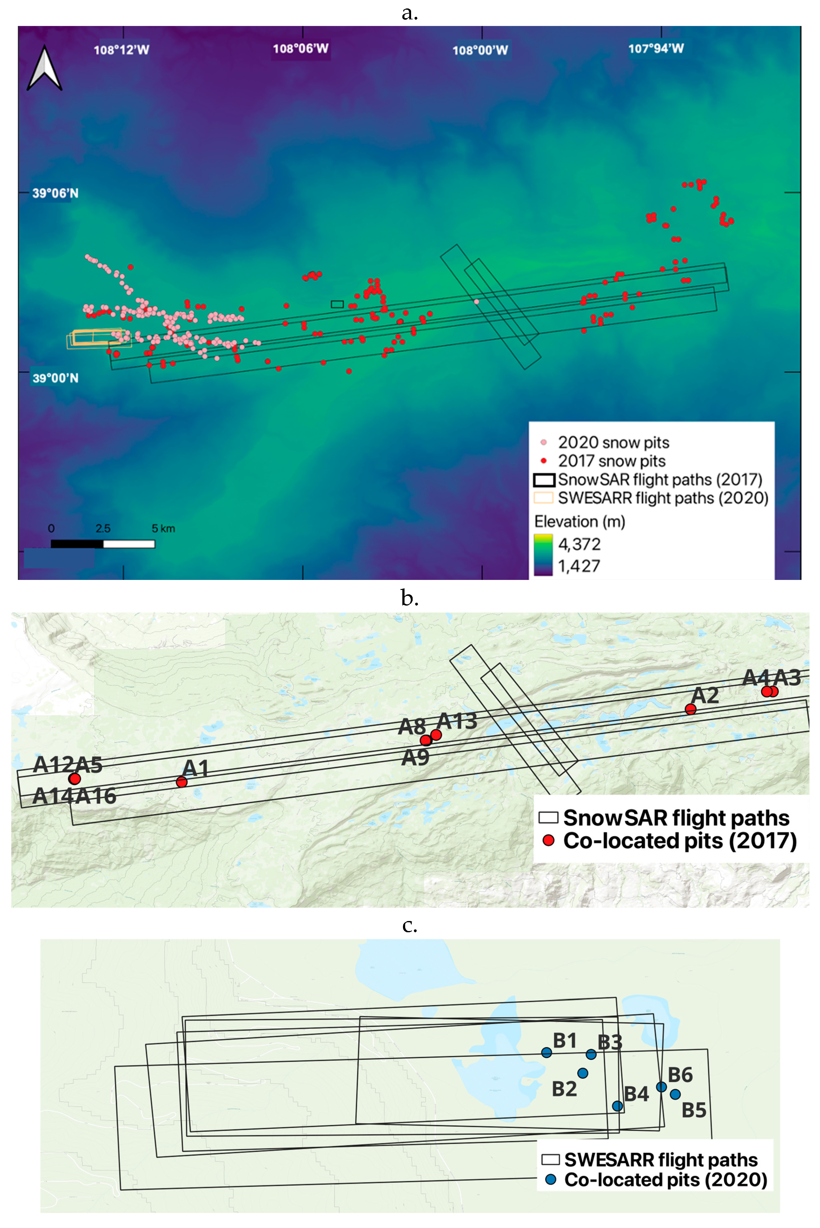
Figure 3.
Flowchart explaining the methodology of (a) Sensitivity analysis and (b) Bayesian MCMC optimization.
Figure 3.
Flowchart explaining the methodology of (a) Sensitivity analysis and (b) Bayesian MCMC optimization.
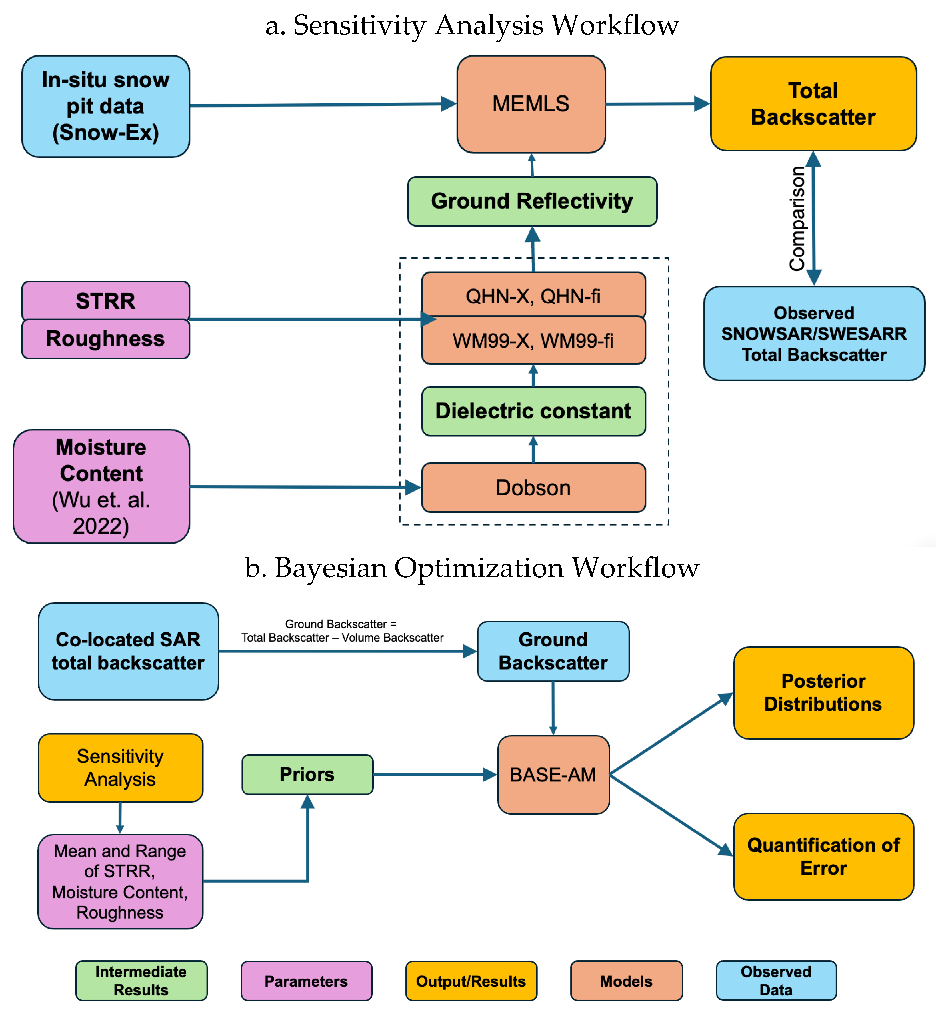
Figure 4.
(a) Bias in average X-VV backscatter over surface roughness 0 to 1.2 cm simulated using each of the 4 soil models with MEMLS (the realizations are mapped using Table A2); (b) RMSE for backscatter simulated using each soil model over the range of surface roughness with QHN-fi as target.
Figure 4.
(a) Bias in average X-VV backscatter over surface roughness 0 to 1.2 cm simulated using each of the 4 soil models with MEMLS (the realizations are mapped using Table A2); (b) RMSE for backscatter simulated using each soil model over the range of surface roughness with QHN-fi as target.
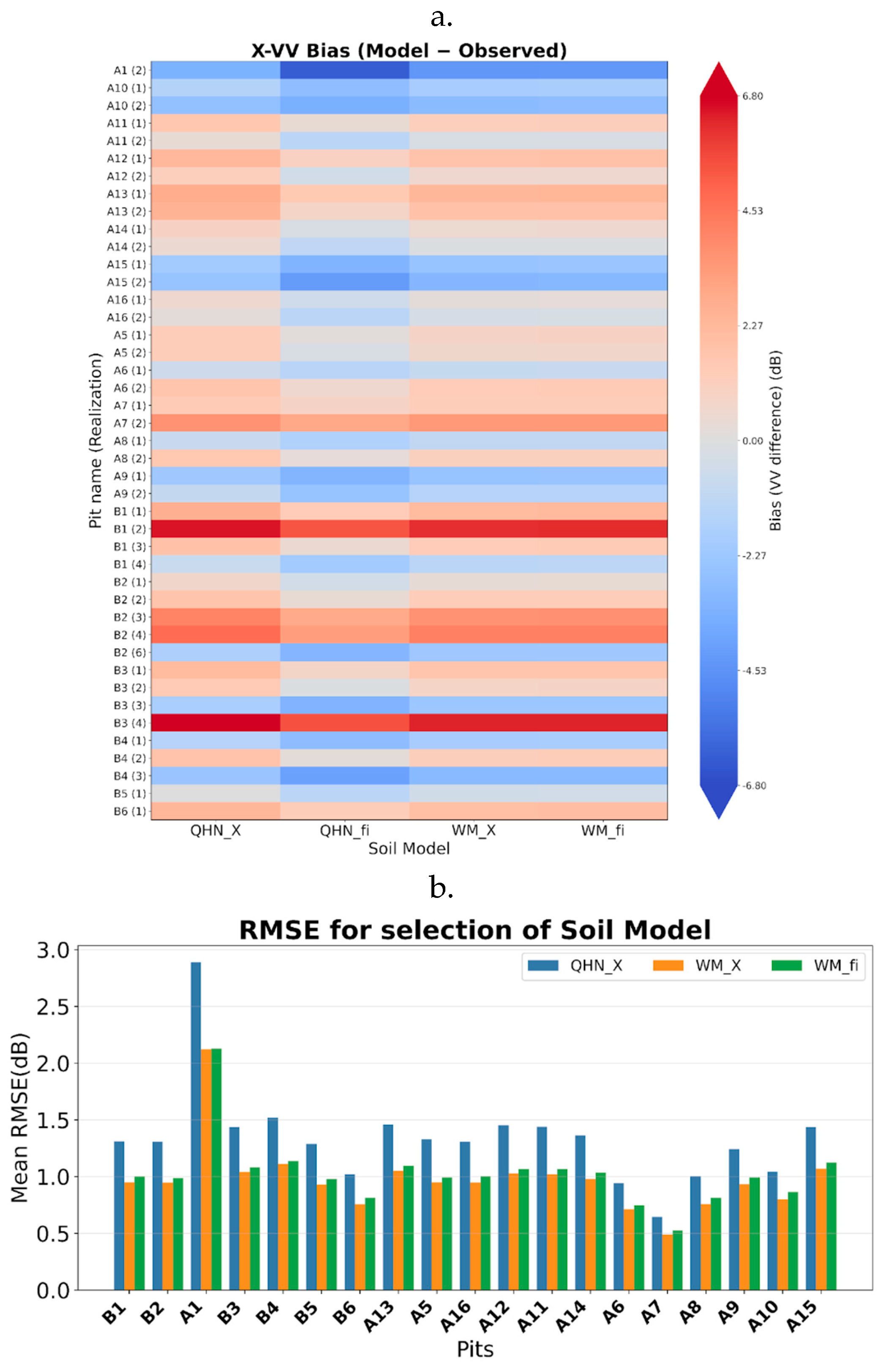
Figure 5.
Sensitivity of LWC in the top 1 cm of the snowpack to the total synthetic backscatter for (a) X-band VV, (b) X-band HH, (c) Ku-band VV. The analysis was carried out for each pit and aggregated into groups of patterns using Euclidean k-means clustering. The dotted line represents the mean of the observed backscatter for each cluster. Refer to Figure S4, S5, S6 for LWC sensitivity analysis for each pit.
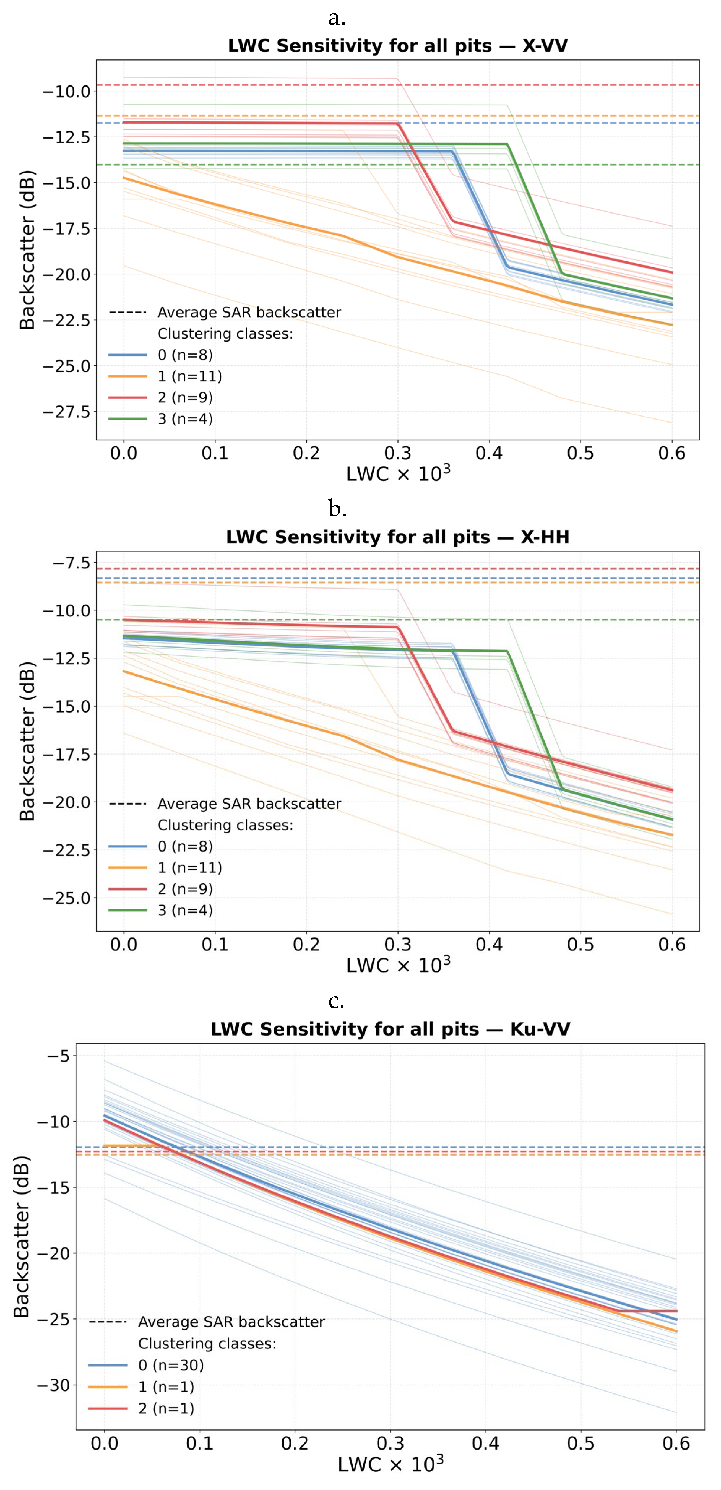
Figure 6.
Examples of Sensitivity Analysis of Ku-band VV backscatter for a range of surface roughness and STRR for 2017 observations (sensitivity analysis for all the pits can be seen in Figure A1).
Figure 6.
Examples of Sensitivity Analysis of Ku-band VV backscatter for a range of surface roughness and STRR for 2017 observations (sensitivity analysis for all the pits can be seen in Figure A1).
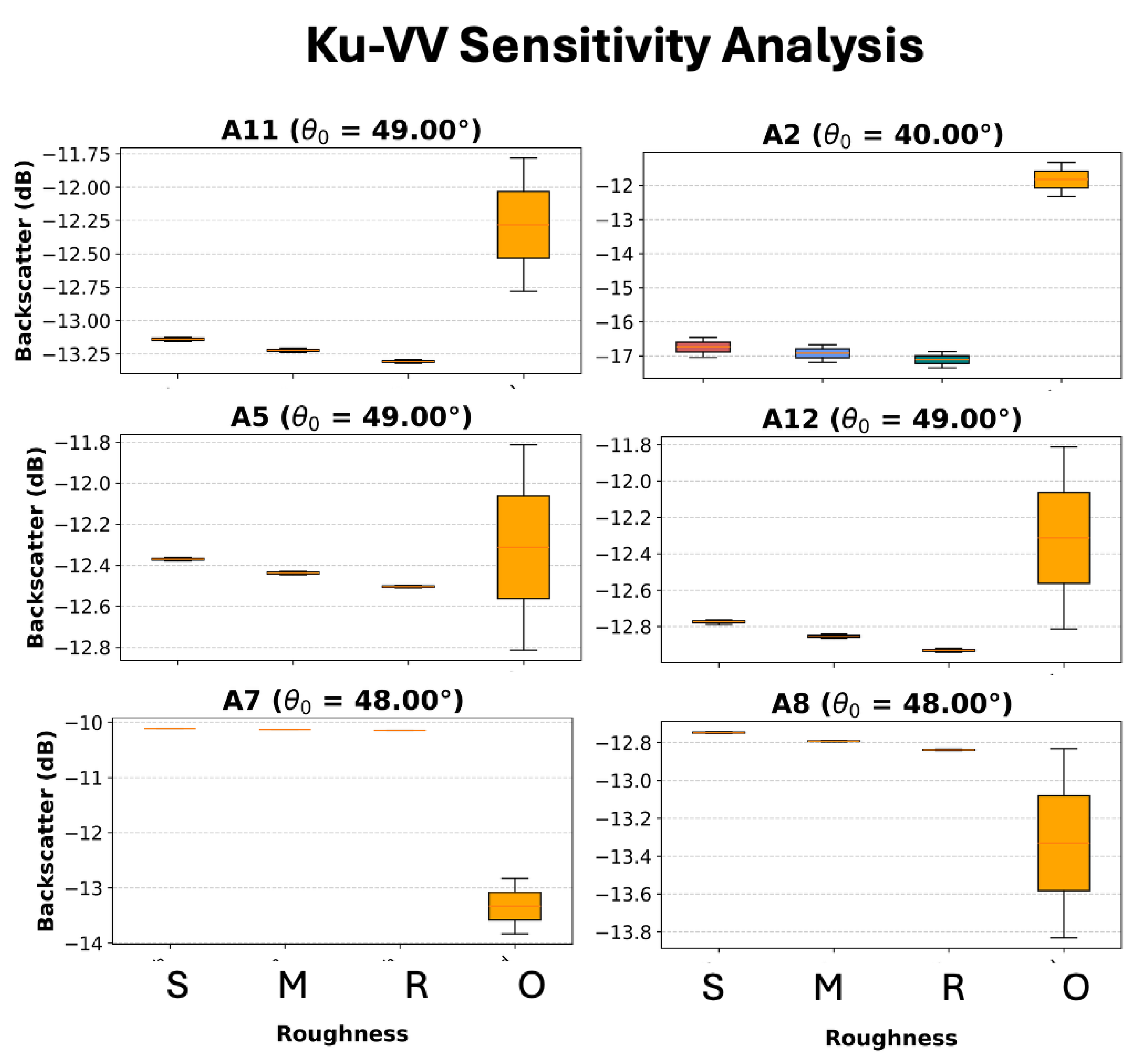
Figure 7.
Examples of Sensitivity Analysis of X-band HH backscatter for a range of surface roughness and STRR for 2017 observations (sensitivity analysis for all the pits can be seen in Figure A2).
Figure 7.
Examples of Sensitivity Analysis of X-band HH backscatter for a range of surface roughness and STRR for 2017 observations (sensitivity analysis for all the pits can be seen in Figure A2).
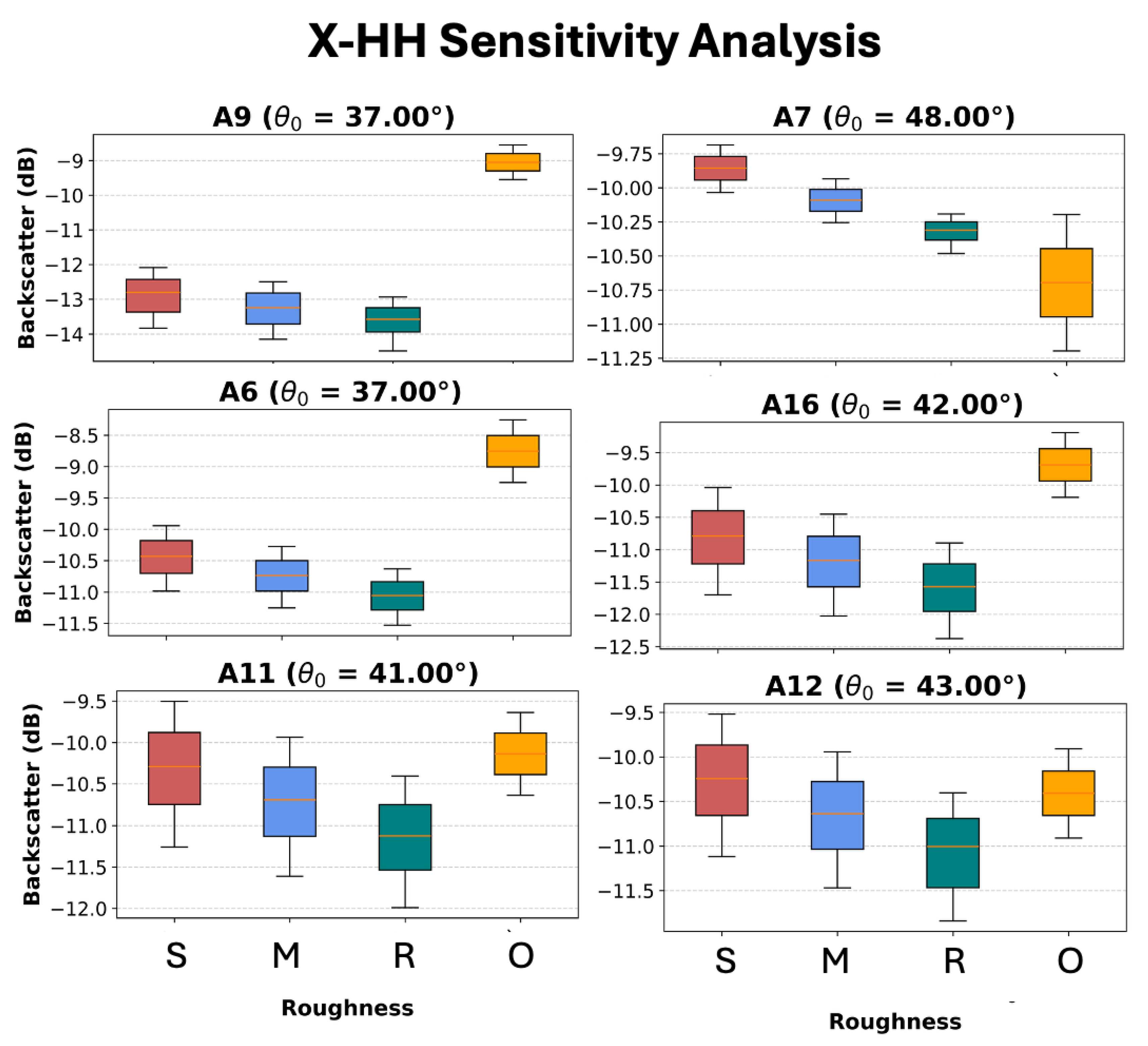
Figure 8.
Examples of Sensitivity Analysis of X-band VV backscatter for a range of surface roughness and STRR for all the observations – 2017 (sensitivity analysis for all the pits can be seen in Figure A3).
Figure 8.
Examples of Sensitivity Analysis of X-band VV backscatter for a range of surface roughness and STRR for all the observations – 2017 (sensitivity analysis for all the pits can be seen in Figure A3).
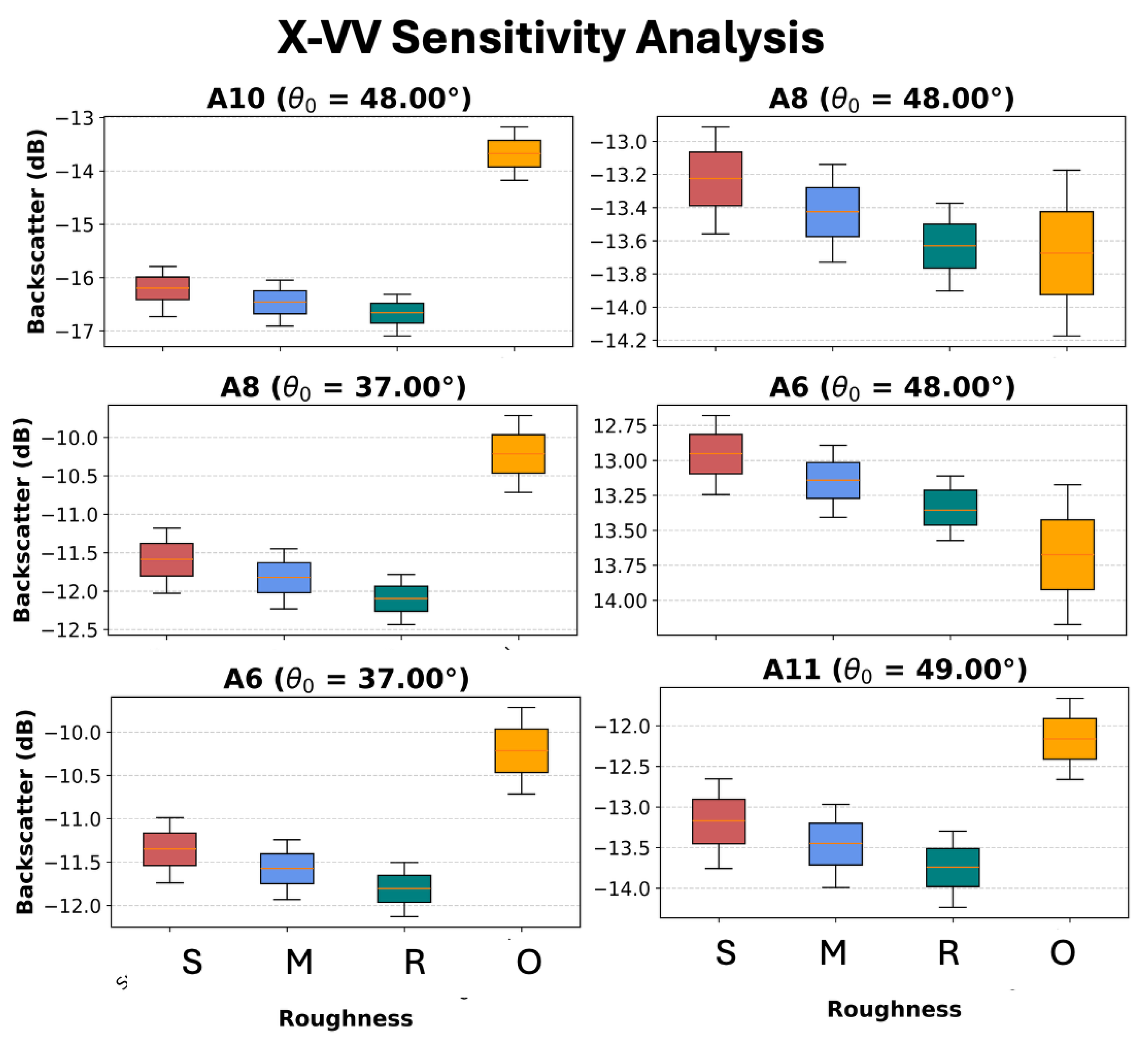
Figure 9.
Sensitivity Analysis of X-band VV backscatter for a range of surface roughness and STRR for all the observations – 2020 (sensitivity analysis for all the pits can be seen in Figure A4).
Figure 9.
Sensitivity Analysis of X-band VV backscatter for a range of surface roughness and STRR for all the observations – 2020 (sensitivity analysis for all the pits can be seen in Figure A4).
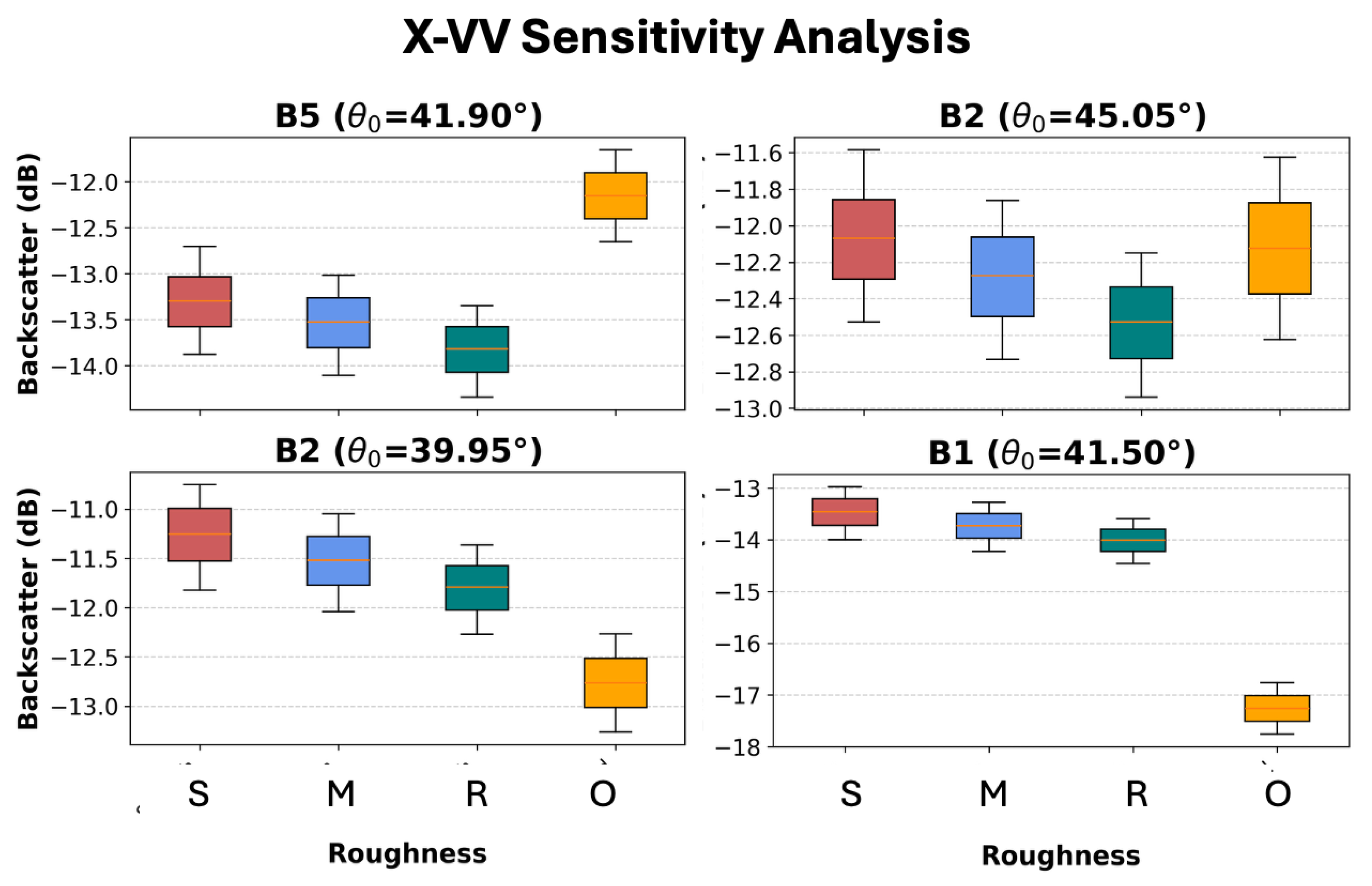
Figure 10.
Posterior distributions when both VV and HH ground backscatter were used for Bayesian optimization. (a) Real part of dielectric constant of the soil calculated using soil moisture that is shown below, (b) STRR, (c) surface roughness, (d) Simulated X-VV and (e) X-HH ground backscatter with red dots representing the observed backscatter with 0.5 dB error bars.
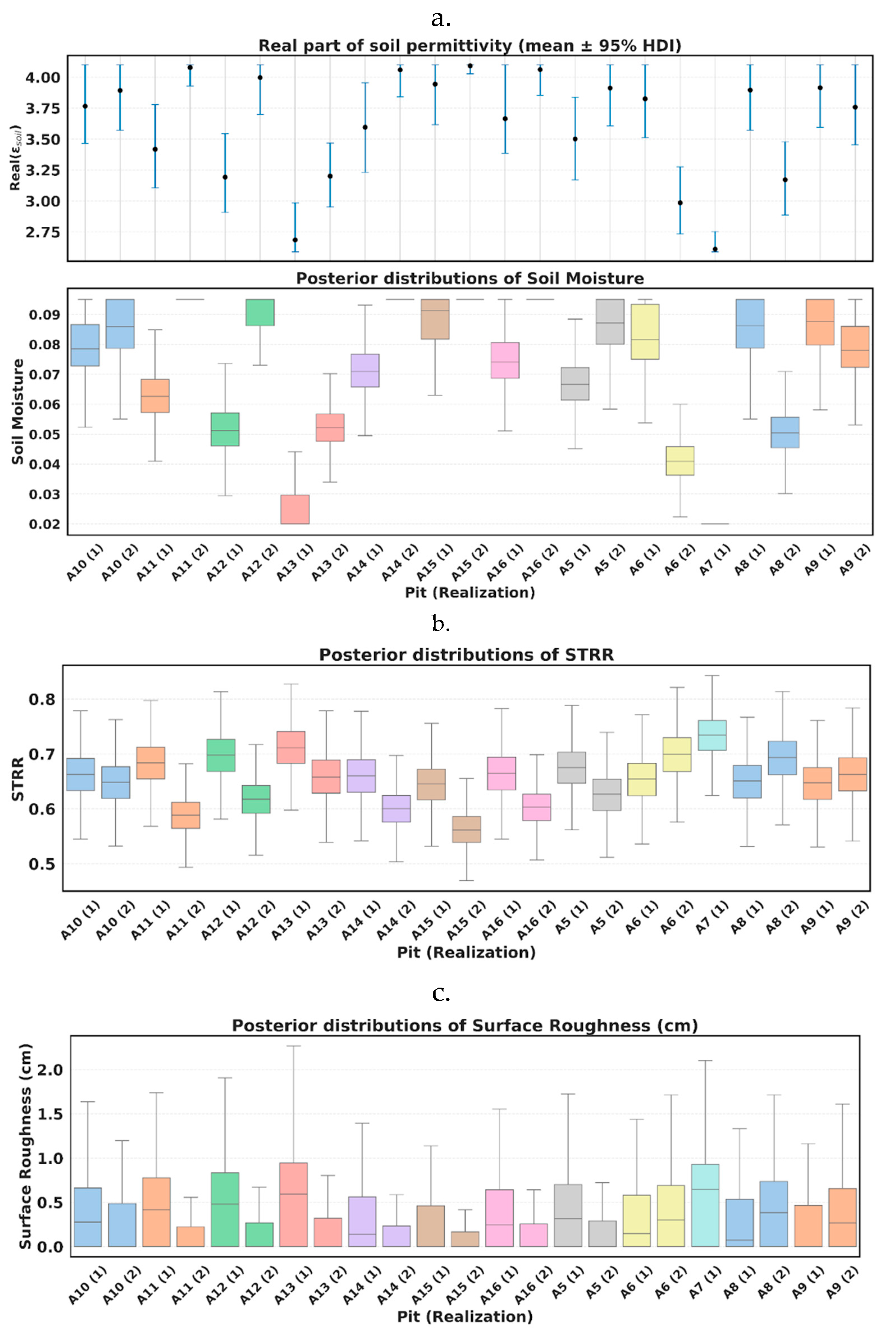
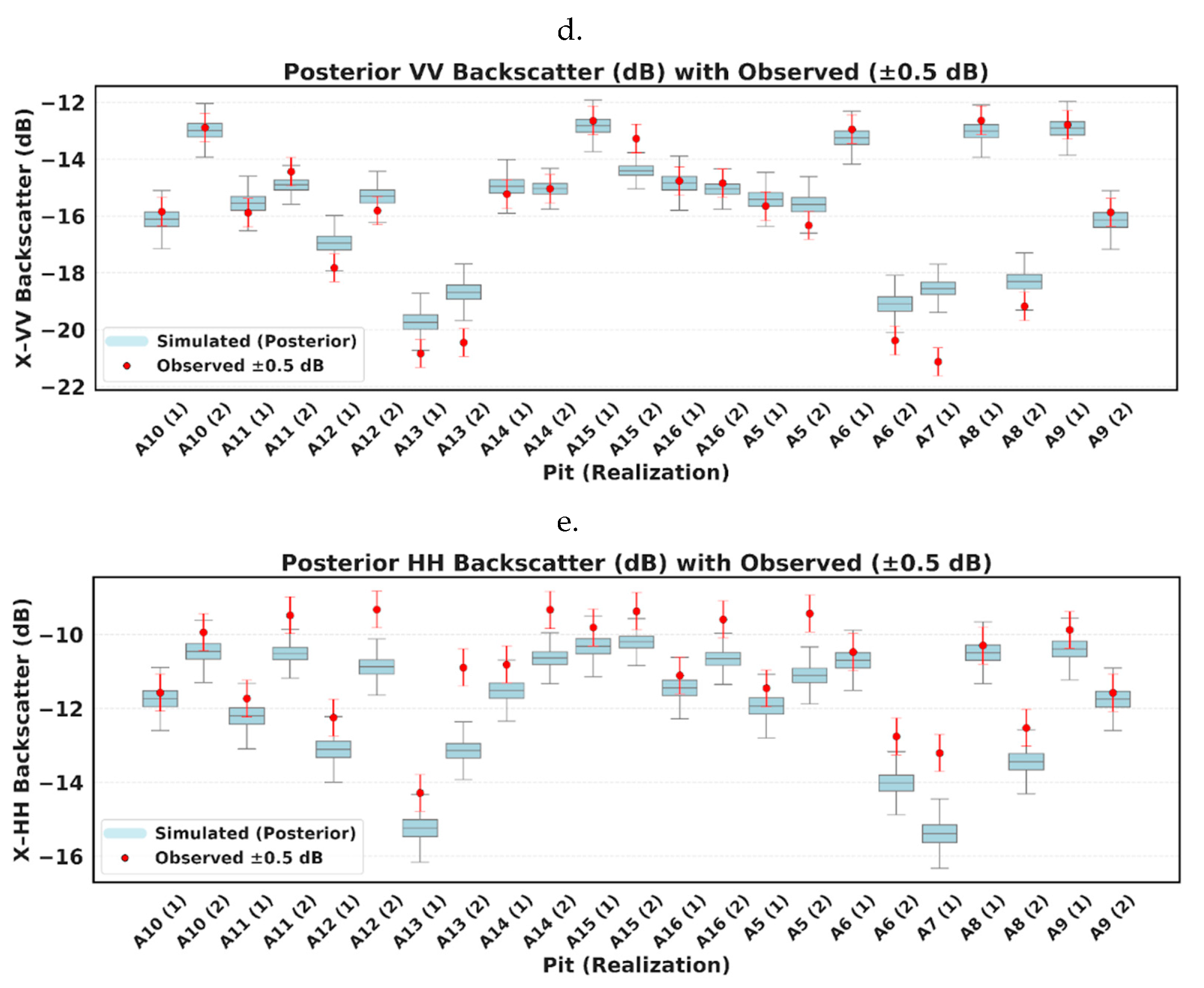
Figure 11.
Posterior distributions when only VV ground backscatter was used for Bayesian optimization. (a) Real part of dielectric constant of the soil calculated using soil moisture that is shown below, (b) STRR, (c) Surface Roughness, (d) Simulated X-VV ground backscatter with red (SNOWSAR) and blue (SWESARR) dots representing the observed backscatter with 0.5 dB error bars.
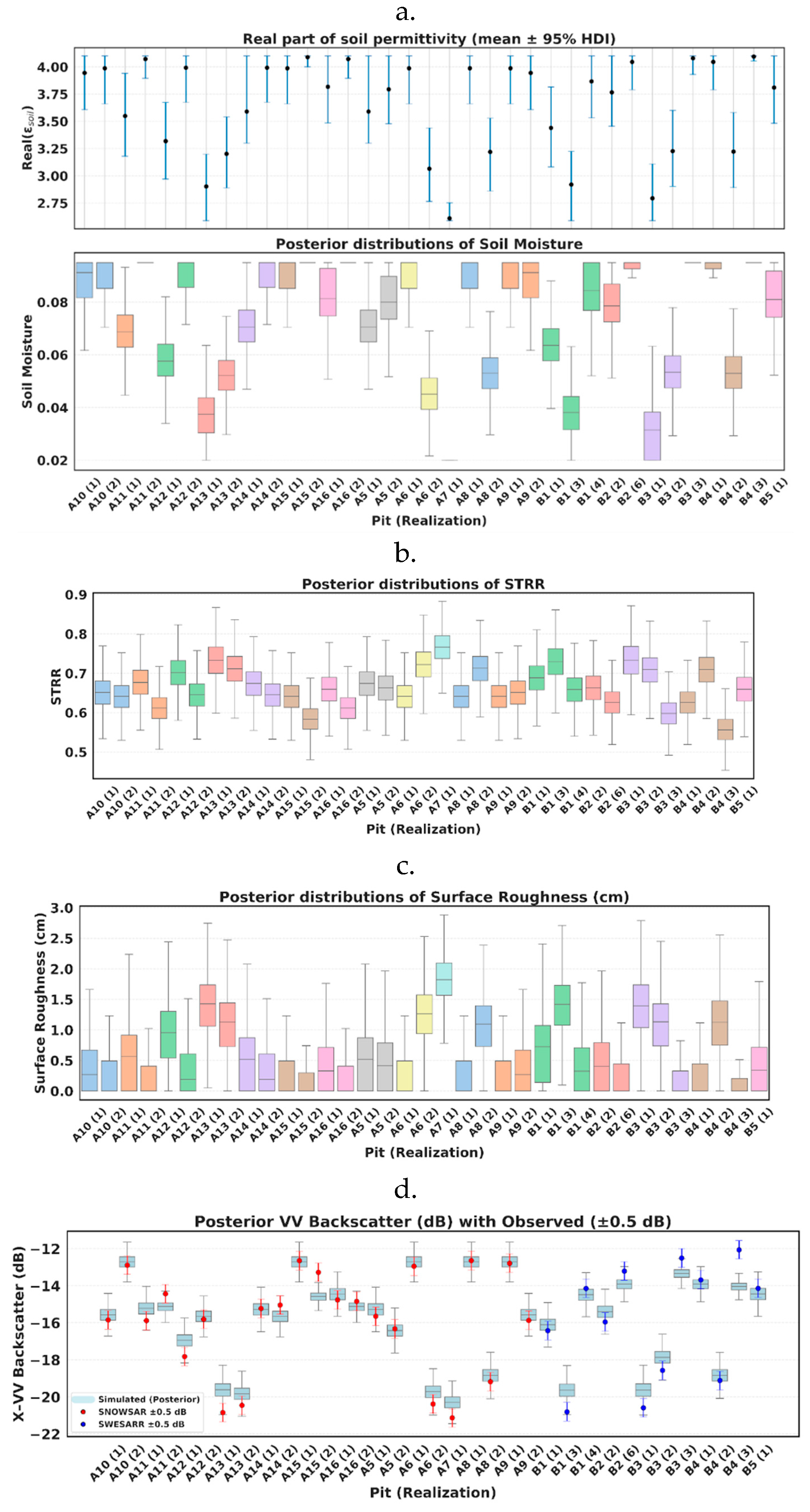
Figure 12.
(a) Standard Deviation in the observed backscatter for each pit when co-located with various resolutions of SAR (1m, 30m, 60m, 90m); (b) Bias in the modeled backscatter vs the standard deviation in the observed backscatter at different resolutions.
Figure 12.
(a) Standard Deviation in the observed backscatter for each pit when co-located with various resolutions of SAR (1m, 30m, 60m, 90m); (b) Bias in the modeled backscatter vs the standard deviation in the observed backscatter at different resolutions.
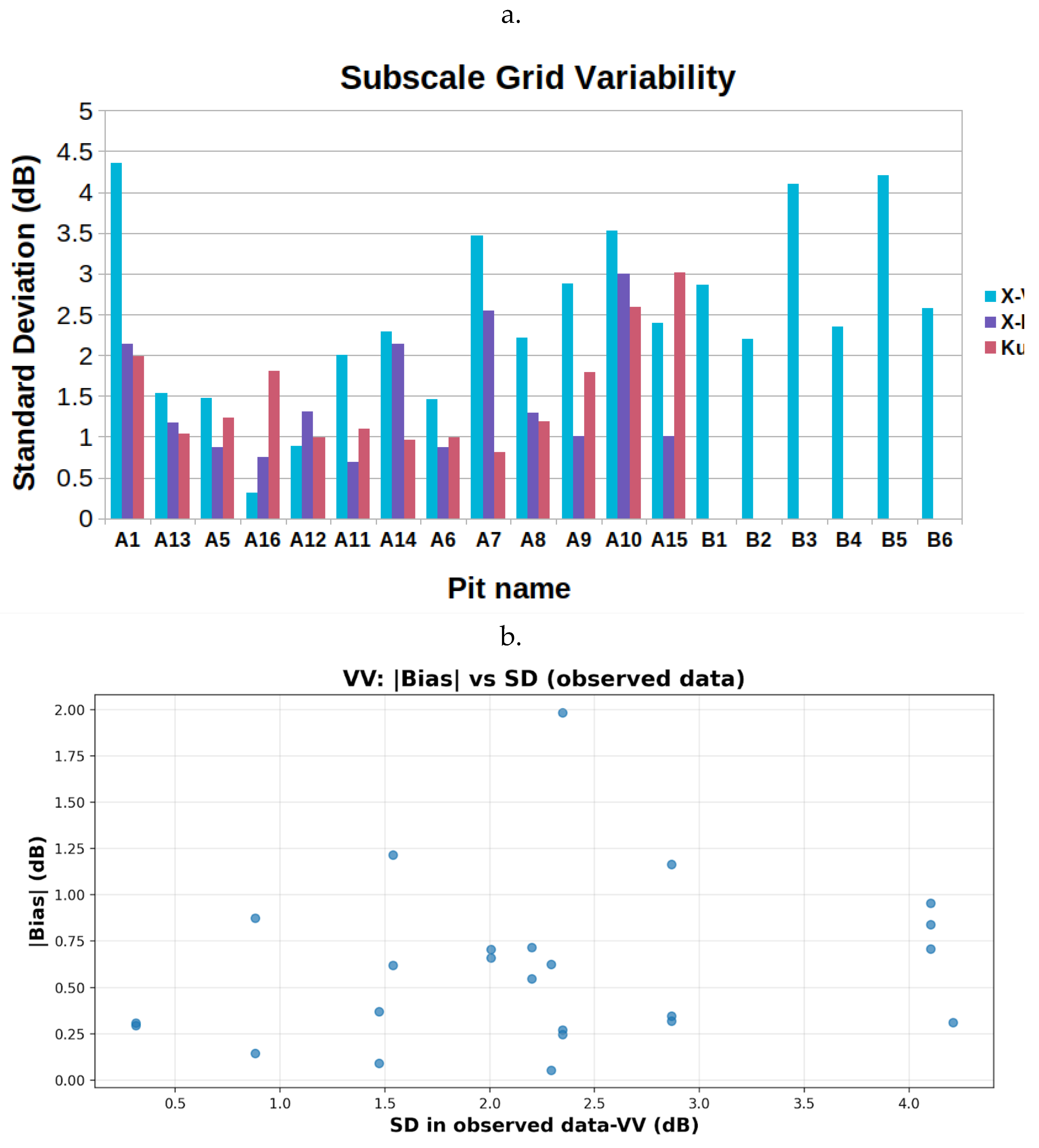
Figure 13.
Bias, surface roughness, and soil moisture content posteriors from Bayesian optimization of multiple synthetic observations at incidence angle of 45° with shaded region representing the 95% HDI for the parameters.
Figure 13.
Bias, surface roughness, and soil moisture content posteriors from Bayesian optimization of multiple synthetic observations at incidence angle of 45° with shaded region representing the 95% HDI for the parameters.
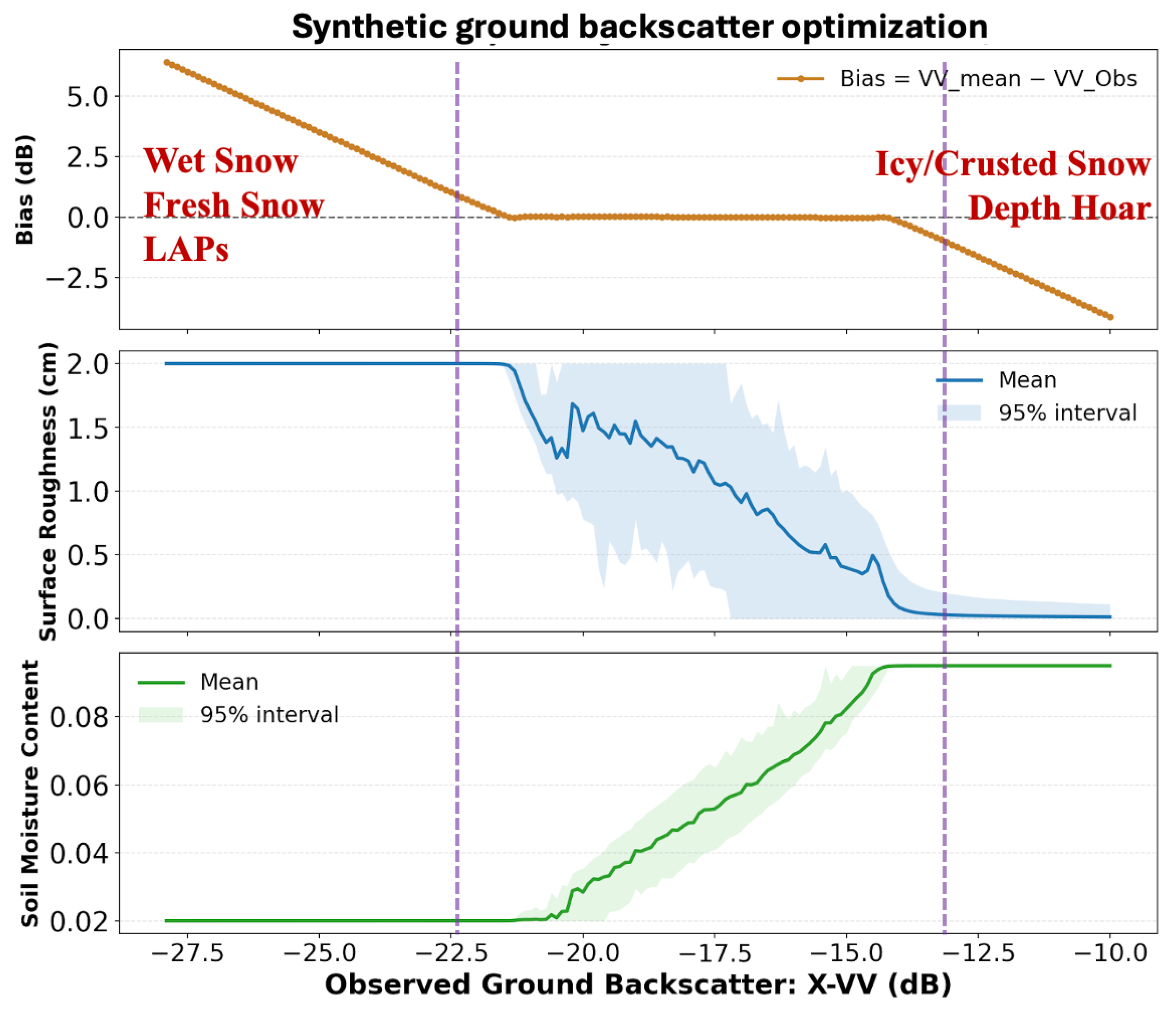
Table 1.
Information of the SAR flights used in this study (SnowSAR and SWESARR -where “F” is frequency, “b” is band and “ΔS” is resolution).
Table 1.
Information of the SAR flights used in this study (SnowSAR and SWESARR -where “F” is frequency, “b” is band and “ΔS” is resolution).
| NSIDC SAR data file naming convention | Flight name (used in the study) | Date | Time (GMT) | Band | Pol | ΔS (m) |
|---|---|---|---|---|---|---|
| 20170221181138<F>G_<b>.nc | 181138 | 2017-02-21 | 18:11:38 | X, Ku | VV, HH | 1 |
| 20170221184320<F>G_<b>.nc | 184320 | 2017-02-21 | 18:43:20 | X, Ku | VV, HH | 1 |
| 20170221185902<F>G_<b>.nc | 185902 | 2017-02-21 | 18:59:02 | X, Ku | VV, HH | 1 |
| 20170221202338<F>G_<b>.nc | 202338 | 2017-02-21 | 20:23:38 | X, Ku | VV, HH | 1 |
| 20170221172126<F>G_<b>.nc | 172126 | 2017-02-21 | 17:21:26 | X, Ku | VV, HH | 1 |
| 20170221173206<F>G_<b>.nc | 173206 | 2017-02-21 | 17:32:06 | X, Ku | VV, HH | 1 |
| GRMST1_27401_20007_005_200211_09225VV_XX_01.tif | 005 | 2020-02-11 | 17:01:07 | X | VV | 1 |
| GRMST1_27702_20007_009_200211_09225VV_XX_01.tif | 009 | 2020-02-11 | 17:25:17 | X | VV | 1 |
| GRMST1_27503_20007_012_200211_09225VV_XX_01.tif | 012 | 2020-02-11 | 17:50:03 | X | VV | 1 |
| GRMST1_27502_20008_025_200212_09225VV_XX_01.tif | 025 | 2020-02-12 | 19:02:37 | X | VV | 1 |
| GRMST1_27021_20008_021_200212_09225VV_XX_01.tif | 021 | 2020-02-12 | 18:38:38 | X | VV | 1 |
| GRMST1_27403_20008_029_200212_09225VV_XX_01.tif | 029 | 2020-02-12 | 19:26:28 | X | VV | 1 |
Table 2.
Co-located snow pits with the observed SAR data that are used in this study (* represents pits whose stratigraphy data were missing and were reconstructed using the nearby pit).
Table 2.
Co-located snow pits with the observed SAR data that are used in this study (* represents pits whose stratigraphy data were missing and were reconstructed using the nearby pit).
| NSDIC Pit name | Pit Name (used in the study) | Latitude | Longitude | Date | Local Time |
|---|---|---|---|---|---|
| 28S | A1 | 39.0122478 | -108.1379938 | 2017-02-25 | 11:00 |
| 78N | A2 | 39.04342878 | -107.9202531 | 2017-02-25 | 15:10 |
| 92E | A3 | 39.0510518 | -107.885109 | 2017-02-22 | 10:00 |
| 92W | A4 | 39.0510159 | -107.8876494 | 2017-02-22 | 13:25 |
| KC1C | A5 | 39.01363394 | -108.1838735 | 2017-02-20 | 10:30 |
| MTR4_0000 | A6 | 39.0300503 | -108.0331353 | 2017-02-24 | 10:15 |
| MTR4_0800 | A7 | 39.03005659 | -108.0332395 | 2017-02-24 | 10:09 |
| MTR4_1390 | A8 | 39.03005509 | -108.0332972 | 2017-02-24 | 10:00 |
| MTR4_2000 | A9 | 39.03005329 | -108.0333664 | 2017-02-24 | 10:08 |
| MTR4_2500 | A10 | 39.03005179 | -108.0334241 | 2017-02-24 | 10:00 |
| KC1S* | A11 | 39.01344468 | -108.1838766 | 2017-02-20 | 12:45 |
| KC1N* | A12 | 39.01381389 | -108.1838816 | 2017-02-20 | 13:00 |
| 67N* | A13 | 39.03245119 | -108.0291492 | 2017-02-22 | 12:20 |
| KC1W* | A14 | 39.01362669 | -108.1841388 | 2017-02-20 | 13:46 |
| MTR4_4500* | A15 | 39.03005478 | -108.0336552 | 2017-02-24 | 10:00 |
| KC1E* | A16 | 39.01363219 | -108.1836079 | 2017-02-20 | 12:30 |
| 1S1 | B1 | 39.02119889 | -108.20559 | 2020-01-29 | 09:05 |
| 1S2 | B2 | 39.019948 | -108.203396 | 2020-02-08 | 09:37 |
| 2S3 | B3 | 39.021089 | -108.202889 | 2020-01-29 | 10:35 |
| 2S4 | B4 | 39.017951 | -108.201292 | 2020-02-05 | 09:30 |
| 2S7 | B5 | 39.01866002 | -108.197788 | 2020-02-08 | 11:35 |
| 3S5 | B6 | 39.01911256 | -108.1986242 | 2020-01-29 | 12:10 |
Table 3.
Values of parameters for the soil dielectric models - WM99 and QHN - as proposed by [36] for frequency independent (fi) and X-band (10.65 GHz).
Table 3.
Values of parameters for the soil dielectric models - WM99 and QHN - as proposed by [36] for frequency independent (fi) and X-band (10.65 GHz).
| Wëgmuller and Mätzler (1999) – WM99 | |||||||||
| f (GHz) | A0 | A2 | A3 | β | Bias | Std | |||
| WM99fi (All) | 0.039 | 0.872 | −0.016 | 2.140 | −0.002 | 0.058 | |||
| 10.65 | 0.080 | 0.935 | 0.302 | 1.890 | −0.012 | 0.052 | |||
| Wang and Chaudhary (1981) – QHN | |||||||||
| f (GHz) | a1 | a2 | a3 | Q | NV | NH | Bias | Std | |
| QHNfi (All) | 0.887 | 0.796 | 3.517 | 0.075 | 1.503 | 0.131 | −0.003 | 0.042 | |
| 10.65 | 0.880 | 0.838 | 3.280 | 0.657 | 3.209 | 0.178 | 0.012 | 0.047 | |
Table 8.
Contribution of the ground backscatter and response of the BASE-AM model for different snowpack classifications.
Table 8.
Contribution of the ground backscatter and response of the BASE-AM model for different snowpack classifications.
| Type | Structure | Total Backscatter | Ground Backscatter Component | BASE-AM observation | ||
|---|---|---|---|---|---|---|
| Fresh snow | Low density (<200 kg/m3), small grains, fluffy, homogeneous. | Low | Weak volume scattering because grains are much smaller than the wavelength (Rayleigh regime) | High | Low density, tiny grains → weak volume; waves reach ground easily | Low observed SAR, overestimating volume, underestimating ground backscatter |
| Depth Hoar (Large Grains, Faceted Snow) | Coarse grains (1–3 mm), low density but with strong internal contrasts | High | X-band is very sensitive here because grain size approaches or exceeds the Rayleigh-to-Mie transition relative to wavelength. Stronger volume scattering than other dry types → higher backscatter. |
Low | Penetration OK, but strong volume scattering from large grains masks ground | High observed SAR, underestimating volume, overestimating ground backscatter |
| Wet Snow (Moisture in Pores, LWC > ~0.5%) | Presence of liquid water between grains, even in small fractions | Very low | Strong absorption and attenuation → backscatter drop sharply. Surface scattering dominates, but the wet snowpack looks darker overall (–15 to –25 dB). Even a thin wet layer on top masks deeper scattering. |
Very low | Liquid water strongly attenuates → ground largely invisible | Low observed SAR, overestimating volume, highly underestimating ground backscatter |
| Snow with Light Absorbing Particles (Dust, Soot, Organic Matter) | Like dry snow but with LAP inclusions | Low | LAPs change dielectric properties slightly and can increase absorption. | Low | LAPs raise absorption slightly → less penetration, hence less ground share | Low observed SAR, overestimating volume backscatter, underestimating ground backscatter |
| Icy or Crusted Snow | Ice lenses, melt-freeze crusts, hard refrozen surfaces. | Very high | Very strong surface scattering at X-band (specular if smooth, diffuse if rough). Appears bright regardless of underlying snow. |
Very low | Crust/ice lenses reflect at shallower depths → cut off penetration | Very high observed SAR, highly underestimating volume backscatter, highly overestimating ground backscatter |
Disclaimer/Publisher’s Note: The statements, opinions and data contained in all publications are solely those of the individual author(s) and contributor(s) and not of MDPI and/or the editor(s). MDPI and/or the editor(s) disclaim responsibility for any injury to people or property resulting from any ideas, methods, instructions or products referred to in the content. |
© 2026 by the authors. Licensee MDPI, Basel, Switzerland. This article is an open access article distributed under the terms and conditions of the Creative Commons Attribution (CC BY) license (http://creativecommons.org/licenses/by/4.0/).
Copyright: This open access article is published under a Creative Commons CC BY 4.0 license, which permit the free download, distribution, and reuse, provided that the author and preprint are cited in any reuse.


