Submitted:
03 January 2026
Posted:
05 January 2026
You are already at the latest version
Abstract
This paper reviews digital floating-point arithmetic algorithms that employ Taylor series expansion combined with mantissa region division techniques, drawing upon the results of our research. In many scientific computing applications, compact and low-power hardware implementations are essential. To address these requirements, this review presents algorithms specifically designed to operate under such constraints. The focus is placed on efficient floating-point operations—including division, inverse square root, square root, exponentiation, and logarithmic functions—all realized through Taylor series expansions. Furthermore, the paper examines the trade-offs involved, such as the number of additions, subtractions, and multiplications, as well as the hardware cost associated with Look-Up Table (LUT) size. These factors are analyzed to identify the most suitable algorithms for engineering applications and to facilitate their practical implementation.
Keywords:
floating-point
; digital arithmetic
; Taylor-series expansion
; mantissa region division
; division
; inverse square root
; square root
; exponential
; logarithm
1. Introduction
Floating-point arithmetic forms the computational backbone of modern digital systems, from general-purpose processors to application-specific integrated circuits (ASICs) and field-programmable gate arrays (FPGAs) [1,2,3]. The increasing demand for high-performance digital signal processing in embedded systems, IoT devices, and edge computing has driven the floating-point operations such as division, inverse square root, square root, exponentiation, and logarithms become increasingly critical in domains including signal processing, control systems, graphics rendering, and machine learning [4,5,6]. However, implementing these operations efficiently on hardware remains a persistent challenge, particularly in systems constrained by area, power, and latency [7,8].
To address these challenges, researchers have explored various approximation techniques for floating-point arithmetic, including polynomial expansions, lookup table (LUT)-based methods, and iterative algorithms [9,10,11]. Among these strategies, Taylor series expansion has emerged as a promising approach for approximating complex mathematical functions in floating-point computation [11,12]. The Taylor series represents a function as an infinite sum of terms calculated from its derivatives at a single point [13]. By truncating the series after a limited number of terms, designers can approximate functions with a controlled balance between accuracy and computational effort [14,15]. The elegance of the Taylor series lies in its polynomial form, enabling efficient realization using elementary arithmetic operations such as addition and multiplication, which are well-supported in hardware design [16,17].
Despite the apparent simplicity of Taylor series-based approximations, applying them directly to floating-point functions presents several challenges. The convergence of a Taylor series can vary significantly across the domain of the target function [18,19]. For instance, a Taylor series approximation of the natural logarithm, ln(x), converges quickly near the expansion point but poorly at values further away [20,21]. To address this, methods such as interpolation based on Taylor series approximation can be used to divide the period into multiple intervals [22]. Additionally, exponential operations can be performed, and an integer part can be added for floating-point arithmetic [23]. These techniques transform or partition the input domain into smaller subregions where the Taylor expansion achieves faster convergence with fewer terms. For LUT optimization, some researchers employ deep neural networks and CORDIC-based integer arithmetic methods, which reduce the number of required arithmetic operations and minimize the size of auxiliary lookup LUTs needed for storing coefficients or intermediate values [24,25].
This review presents recent advances in floating-point algorithms for division, inverse square root, square root, and exponentiation, developed using Taylor series expansion techniques and informed by our research findings [12,27,28,29,30]. Specifically, it highlights techniques that optimize the trade-offs among the number of additions/subtractions, and multiplications and the size of LUTs in hardware implementations. These algorithms aim to deliver compact, low-power solutions suitable for modern embedded and portable systems where hardware resources are at a premium.
This paper is organized as follows. Section 2 reviews related work. Section 3 provides the necessary background, including the Taylor series expansion, the representation of floating-point numbers, and the mantissa division method for Taylor series expansion. Section 4 through 9 present floating-point computation algorithms based on Taylor series expansion with mantissa division, covering division, inverse square root, square root, exponentiation, and logarithm calculations, respectively. Finally, Section 10 concludes the paper.
2. Related Works
A number of recent studies have advanced the application of Taylor series expansion in floating-point arithmetic to achieve high precision with reduced hardware resource requirements. When employing Taylor series expansion for high-precision floating-point computations, critical trade-offs must be balanced among computational accuracy (minimizing polynomial terms), hardware resource efficiency (reducing LUT requirements), and implementation complexity. This paper presents a comprehensive analysis of these design constraints and introduces a divide-and-conquer implementation of Taylor series approximation for optimized floating-point arithmetic.
2.1. Motivation for Taylor-Series-Based Floating-Point Arithmetic
Floating-point operations are traditionally performed using well-established techniques such as digit-recurrence methods (e.g., SRT division for division and square root) or iterative refinement approaches (e.g., Newton-Raphson or Goldschmidt’s methods for division and reciprocal square root). While these methods offer high precision, they often require multiple cycles of computation and complex control logic, making them less attractive for resource-constrained applications.
Taylor series expansion provides an alternative that replaces iterative or digit-wise computation with polynomial evaluation [9,15]. Since polynomials can be evaluated efficiently using Horner’s rule [26] or similar schemes, the arithmetic operations can be mapped to simple, fast combinational circuits or low-latency pipelines [13,17]. This makes Taylor series expansion particularly attractive for hardware accelerators and embedded processors [9].
However, direct application of Taylor series faces limitations, as convergence depends heavily on the domain of input values [18,20]. For example, a Taylor series centered at 1.0 provides an excellent approximation for ln(x) when x is close to 1.0 but performs poorly as x deviates from this point [21]. Thus, domain segmentation strategies are essential to ensure that approximations remain accurate across the entire input space.
2.2. Mantissa Region Division Technique
To extend the applicability of Taylor series to floating-point arithmetic, mantissa region division methods are described in this review. This technique divides the mantissa domain into smaller subregions where the approximation error remains within acceptable bounds using low-order polynomials.
Other arithmetic, a divide-and-conquer approach was introduced, where the input domain is recursively partitioned and each subdomain approximated individually using tailored Taylor expansions. These methods, combined with optimal domain division strategies, offer a powerful toolkit for floating-point function realization on hardware.
2.3. Balancing LUT Size and Arithmetic Complexity
A key advantage of Taylor series-based methods is their potential to reduce reliance on large LUTs. Traditional LUT-based methods for transcendental functions often consume significant memory, particularly when high precision is required across a broad domain. By using domain segmentation and low-order polynomials, Taylor series-based designs can achieve similar precision with smaller LUTs that only store coefficients or domain-specific parameters.
At the same time, designers must carefully balance LUT size with the number of arithmetic operations required. A lower-order Taylor polynomial reduces multiplications but may require more domain partitions (and thus more LUT entries). Conversely, a higher-order polynomial reduces the need for domain segmentation but increases the number of arithmetic operations. Exploring these trade-offs is essential for achieving optimal designs, especially in power- and area-constrained environments.
2.4. Comparative Analysis and Hardware Trade-Offs
The reviewed algorithms demonstrate that Taylor-series expansion, when combined with smart domain partitioning and LUT optimization, can achieve high precision with reduced hardware complexity. The primary trade-offs include:
- LUT size vs. arithmetic operations: Larger LUTs reduce polynomial order but increase memory usage.
- Number of segments vs. approximation error: Finer segmentation improves accuracy but requires more comparators and control logic.
- Multiplier complexity vs. latency: Higher-order polynomials need more multipliers but may reduce iteration counts.
These insights are crucial for hardware designers aiming to implement energy-efficient floating-point units in ASICs or FPGAs.
3. Preparation
3.1. Taylor Series Expansion
Let be an infinitely differentiable function. Its Taylor series expansion about the point x = a is given by:
Many functions commonly used in engineering design exhibit a relatively wide radius of convergence. As the order n increases, their Taylor series expansions approach over a broad range of x. For example, the Taylor series expansions centered at a = 0 for functions such as sine and cosine for -∞ < x < ∞, respectively, as n increases (Figure 1).
To the best of our knowledge, there are very few algorithms in engineering that effectively leverage the fact that the Taylor series expansion of certain functions converges to across a broad domain of x . In this paper, we review digital floating-point arithmetic algorithms used to compute division, inverse square roots, square roots, exponential functions, and logarithms, based on Taylor series expansion.
3.2. Representation of Floating-point Numbers
Consider the binary representation of floating-point numbers.
Mantissa : M
Exponent : E
Binary representation : x
Mantissa (Here… is 0 or 1)
Note that the binary point is placed such that 1≤ M <2. For example, M=1.011001(binary) = 1.390625 (decimal). As shown in Figure 2, the IEEE-754 format represents a floating-point number using three components: the sign bit (S), the exponent (E), and the mantissa (M).
The IEEE 754 standard includes double-precision (64-bit), single-precision (32-bit), and half-precision (16-bit) formats, and the level of precision can be chosen by the system designer.
In this paper, we focus primarily on cases where the sign bit is positive. A binary floating-point number, denoted as X , consists mainly of an exponent part and a mantissa part, represented by E and M respectively. The following equation expresses this relationship:
In this context, the floating-point mantissa is expressed as M = 1. …, where , etc., are binary digits (each either 0 or 1). The value of M falls within the range 1 ≤ M < 2. For example, M = 1.01111 in binary corresponds to 1.46875 in decimal.
3.3. Mantissa Division Method for Taylor Series Expansion
n this subsection, we introduce the uniform mantissa segmentation technique for Taylor series expansion. As the number of segments increases, fewer Taylor series terms are required to achieve the specified accuracy.
Simulations have been conducted to determine the number of Taylor series expansion terms, n, required for , across various accuracy levels and target regions, satisfying the following conditions:
Here, represents the ideal value of functions such as the reciprocal, inverse square root, square root, exponentiation or logarithm. denotes the Taylor expansion approximation using n terms, and indicates the target accuracy for all x within the specified region.
3.3.1. One Mantissa Region for Taylor-Series Expansion
There is no region in the divide 1 ≤ x < 2. The central value a is defined as 1.5, as shown in Table 1.
3.3.2. Division by 2 of Mantissa Region 1≤x<2
Divide the region 1≤x<2 by 2 and select one, based on M as shown in Table 2. Then perform the Taylor-series expansion at the center point a of the chosen region.
3.3.3. Division by 4 of Mantissa Region 1 ≤ x < 2
Divide the region 1 ≤ x< 2 by 4 and select one, based on M as shown in Table 3. Then perform the Taylor-series expansion at the center point a of the chosen region.
3.3.4. Division by 8 of Mantissa Region 1≤x<2
Divide the region 1≤x<2 by 8 and select one, based on M as shown in Table 4. Then perform the Taylor-series expansion at the center point a of the chosen region.
In the subsequent sections, we apply the above segmentation method to division, inverse square root, square root, exponential, and logarithmic algorithms using Taylor series expansion, in order to determine the minimum number of expansion terms required to achieve a given precision. Moreover, we emphasize the trade-offs involved in the number of additions/subtractions, and multiplications, as well as the size of the LUTs required in hardware. These factors are analyzed to identify the most suitable algorithms for engineering applications and to support their practical implementation.
4. Division Algorithm Using Taylor Series Expansion
4.1. Introduction
This section introduces floating-point division algorithms using Taylor series expansion with uniform mantissa division [27].
Typical applications of floating-point division in digital processors are as follows: (i) Computer Graphics (Rendering): Used in pixel color calculations and light reflection models, where ratios and normalization require division; (ii) Digital Signal Processing: Audio and image filtering often involve normalization coefficients or gain adjustments that rely on division; (iii) Machine Learning & AI: Neural network training uses division for learning rate adjustments and normalization, especially in batch normalization and probability distribution calculations; (iv) Physics Simulations (Games & Scientific Computing): Fundamental formulas like velocity = distance ÷ time or density = mass ÷ volume depend on division; (v) Financial Calculations: Ratios such as exchange rates or interest rates require division. Example: profit margin = profit ÷ investment; (vi) Image Processing (Computer Vision): Histogram normalization and brightness correction often divide pixel values by maximum or average values; (vii) Numerical Analysis in Engineering: Division is essential in linear algebra (matrix inversion, Gaussian elimination) and in simulations like finite element methods or fluid dynamics.
In short, floating-point division is indispensable whenever ratios, normalization, or distribution calculations are needed — spanning graphics, AI, physics, finance, vision, and engineering.
4.2. Problem Formulation
Let us consider a division algorithm that calculates A=N/D for three numbers A, N and D in binary floating-point representation, where A, N and D are expressed as follows:
Once 1/D is computed, A = N/D can be obtained using a standard digital multiplication algorithm.
Since 1/D = , calculating the reciprocal of the mantissa (is the key step in obtaining 1/D. Therefore, we study an algorithm that performs the Taylor series expansion of f(x)=1/x and computes its approximation with a specified degree of accuracy.
4.3. Reciprocal Calculation by Taylor-Series Expansion
Let us consider the calculation of (1 ≤ < 2) using Taylor-series expansion of , centered at x=a (1 ≤ a <2), to achieve the desired accuracy. Taylor expansion of at x=a is as follows:
Here, .
Note that each term has a coefficient of either +1 or -1 for y, which simplifies the calculation by minimizing the number of multiplications.
4.4. Numerical Simulation Results
In this subsection, simulations are employed to determine the number of terms (n) required for the Taylor-series expansion of under various conditions of given accuracies and regions.
4.4.1. One Mantissa Region of
Table 5 shows the required number of the terms n for Taylor-series expansion to meet the desired accuracy, obtained by numerical simulation.
4.4.2. Division by 2 of Mantissa Region
4.4.3. Division by 4 of Mantissa Region
4.4.4. Division by 8 of Mantissa Region
4.5. Hardware Implementation Consideration
Consider the complexity of hardware implementation for computing the reciprocal of using the examined algorithm.
4.5.1. SRequired Numbers of Multiplications/Additions/ Subtractions for Taylor-Series Expansion
Example 1: Five terms of Taylor-Series expansion case
Let us consider to calculate the following with multiplier, adder/subtracter and LUT.
where a is a constant and x is a variable. 1/a is calculated in advance and stored in LUT memory, which is read for the calculation. Then we calculate and . Next, we calculate the followings:
We see that can be obtained with 4 multiplications and 4 additions/subtractions.
We see from Table 8 and Table 9 that by dividing the region by 8, the reciprocal of the mantissa can be calculated with 20-bit accuracy by 4 multiplications and 4 additions/subtractions.
Example 2: Seven terms of Taylor-Series expansion case
Next, let us consider the following:
Similarly, (1/a) is read from LUT and we calculate y=(x-a)/a (=(1/a)x – 1) and z=. Then we calculate the following:
We see that can be obtained with 5 multiplications and 5 additions/subtractions.
Table 9 shows the required numbers of multiplications and additions/subtractions for the number of Taylor-series terms for .
4.5.3. LUT Contents and Size
The value of 1/a is precomputed and stored in memory for later use during the Taylor-series calculation. When the region is divided into four parts, a 4-word LUT is required, as illustrated in Table 10. The data corresponding to the address is accessed for =1.…. It should be noted that LUT addressing is straightforward since an address decoder is not needed.
4.6. Summary of Division Algorithm Part
We have introduced floating-point division algorithms utilizing the Taylor-series expansion of with mantissa region division method. It highlights the hardware implementation trade-offs, including division accuracy, the number of multiplications, additions, subtractions, and LUT sizes, enabling flexibility to meet diverse digital division specifications. As the number of mantissa region divisions increases, the number of multiplications, additions, and subtractions decreases, while the LUT size increases.
5. Inverse Square Root Algorithm Using Taylor Series Expansion
5.1. Introduction
This section introduces floating-point inverse square root algorithms using Taylor series expansion with uniform mantissa division [28].
Typical applications of floating-point inverse square root are as follows: (i) Computer Graphics & 3D Rendering: Used for vector normalization (e.g., calculating unit vectors for lighting, shading, and camera transformations). (ii) Physics Simulations in Games: Essential for computing distances and normalizing velocity vectors quickly, improving real-time performance. (iii) Machine Learning & AI: Appears in optimization algorithms and normalization steps where inverse square roots stabilize variance scaling. (iv) Robotics & Control Systems: Used in orientation calculations (e.g., quaternion normalization) for stable motion control. (v) Digital Signal Processing: Applied in RMS normalization and energy scaling, where inverse square roots help adjust signal magnitudes efficiently. (vi) Computer Vision & Image Processing: Used in feature extraction and normalization of gradient vectors (e.g., in edge detection or SIFT descriptors). (vii) Scientific & Engineering Computations: Appears in numerical methods requiring normalized vectors, such as finite element analysis, fluid dynamics, and electromagnetics.
In short, inverse square root is a performance-critical shortcut for normalization tasks across graphics, physics, AI, robotics, DSP, vision, and engineering.
5.2. Representation and Computation of Floating-Point Inverse Square Roots
Let us now consider a floating-point algorithm designed to compute the inverse square root of a binary floating-point number, denoted as Isq:
Here, we examine the exponent by considering separate cases where the exponent E is either even or odd.
When is even, let , and the following can be obtained:
We obtain the exponent part and the mantissa part of . After further normalizing the floating-point type of , the following is obtained:
Since , thenand hence . We have the following:
where, and are the mantissa part and the exponent part of , respectively.
When E is odd, let , and the following is obtained:
After normalizing the floating-point type of , the following is obtained:
Since , then , which leads to , we have the following:
where, and are the mantissa part and the exponent part of , respectively.
5.3. Taylor-Series Expansion of Inverse Square Root
When and the center value is a, we obtain the following equation:
5.4. Number Simulation Results
Now we discuss how to achieve the specified precision by employing the minimal number of Taylor series expansion terms required for computation under the given accuracy constraints.
5.4.1. One Mantissa Region of (Table 1)
Table 11 shows the required number of the terms n for Taylor-series expansion to meet the desired accuracy, obtained by numerical simulation.
5.4.2. Division by 2 of Mantissa Region
5.4.3. Division by 4 of Mantissa Region
5.4.4. Division by 8 of Mantissa Region
5.5. Hardware Implementation Consideration
Let us analyze the hardware implementation complexity of the algorithm under study for computing across different scenarios. Specifically, we examine the number of required multiplications, additions, and subtractions involved in using a Taylor series expansion to compute . For instance, when employing a 5-term Taylor series expansion for centered at a given point a , we obtain the following:
(1)In case that is an even number ():
Let, and .
Here, .
(2)In case that E is an odd number ():
Let, and .
Eq. (22) is also defined as follows. Here, for k = 0 , 1 , 2 , 3 , 4 , where a is a constant and x is a variable. The values and are precomputed and stored in the LUT memory, and are accessed during runtime.
Then we calculate , and we have the following:
It can be observed that is computed using 5 multiplications and 5 additions/subtractions. Table V summarizes the number of multiplications and additions/subtractions required for varying numbers of Taylor series terms when approximating. From Table 15 and Table 16, it can be concluded that dividing the inverse square root domain into 8 regions allows the reciprocal of the mantissa to be computed with 24-bit precision using only 5 multiplications and 5 additions/subtractions.
The required LUT size for N regions is N × 10 words. For the case of M=1..., the most significant bit (MSB) and the second MSB are used to address the LUT entry . Table VI presents the case where N = 4 , resulting in an LUT size of 40 words. It should be noted that LUT addressing is straightforward since an address decoder is not needed.
5.6. Summary of Inverter Square Root Algorithm Part
We have reviewed floating-point inverse square root algorithms based on Taylor series expansion with segmented regions, and shown their hardware implementation trade-offs in terms of simulation accuracy, the number of required multiplications, additions/subtractions, and LUT size, providing flexible support for various digital inverse square root specifications. Based on the findings presented in this paper, we assert that designers can construct conceptual, dedicated hardware architectures for inverse square root computation.
6. Square Root Algorithm Using Taylor Series Expansion
6.1. Introduction
This section introduces floating-point square root algorithms using Taylor series expansion with uniform mantissa division [29].
Typical applications of floating-point square root operations are as follows: (i) Computer Graphics & 3D Rendering: Square roots are used in vector normalization (e.g., calculating unit vectors for lighting and shading). (ii) Digital Signal Processing: In audio and image processing, square roots appear in RMS (Root Mean Square) calculations for measuring signal strength. (iii) Machine Learning & AI: Algorithms like gradient descent often use square roots in optimization methods (e.g., RMSProp, Adam optimizers). (iv) Physics Simulations & Games: Square roots are needed for distance calculations (e.g., Euclidean distance in 3D space) and solving equations of motion. (v) Statistics & Data Analysis: Standard deviation and variance calculations require square roots to measure data spread. (vi) Engineering & Scientific Computing: Square roots are essential in solving quadratic equations, wave equations, and numerical methods in structural or fluid analysis. (vii) Cryptography & Security: Certain algorithms (e.g., modular arithmetic, elliptic curve cryptography) involve square root operations in finite fields.
In short, square root operations are indispensable in geometry, optimization, signal measurement, statistical analysis, and cryptography - making them one of the most widely used floating-point functions in digital processors.
6.2. Problem Formulation
A floating-point number is typically composed of a mantissa, a sign bit, and an exponent. In this section, we focus on cases where the mantissa is positive. For clarity, we denote the binary exponent field, the mantissa field, and the overall binary floating-point representation as E, M, and X, respectively, as follows:
Here, the mantissa field is represented as M=1. …, where each of …, etc., is either 0 or 1. For binary floating-point numbers, the mantissa falls within the range 1 ≤ M < 2.
To compute the square root in binary floating-point arithmetic, we can use the following expression:
In the following, we will examine cases where the exponent part E of a floating-point number is either an odd or an even value.
When the exponent of a floating-point number is even, let . This leads to the following result:
Through calculation, the square root result can be separated into an exponent part k and a mantissa part . By normalizing , we obtain the following expression:
Since , thenand hence. We have the following:
We obtain the exponent part k and mantissa part of the final expansion of Sr.
When the exponent E of a floating-point number is odd, let E = 2k + 1. It can then be expressed as follows:
Let be used to normalize the floating-point number, resulting in the following expression:
Since , it follows that , which implies ≤ and Based on this, we derive the following:
We obtain the exponent part k and the mantissa part from the final expansion of Sr.
6.3. Taylor-Series Expansion of Square Root
To compute the square root of the mantissa M using a Taylor series expansion, let , where x = a and 1 ≤ a < 2 . The Taylor series expansion centered at x = a is given as follows:
6.4. Numerical Simulation Results
n the following, we examine the relationship between the function , the number of terms used in its Taylor series expansion, and the resulting approximation accuracy.
6.4.1. One Mantissa Region of (Table 1)
6.4.2. Division by 2 of Mantissa Region
6.4.3. Division by 4 of Mantissa Region
6.4.4. Division by 8 of Mantissa Region
6.5. Hardware Implementation Consideration
We examine the hardware complexity of the algorithm described here. Consider the equation , and evaluate the number of additions, subtractions, and multiplications required when using the Taylor series expansion. For instance, in the case of the 5-term Taylor series expansion for at , we have the following:
Here:We also define as follows:
Here, If is an even number (): and .
If E is an odd number (): and In Eq. (34), x and a represent a variable and a constant, respectively. The coefficients α₀, α₂, α₃, α₄ and β₀, β₂, β₃, β₄ are individually stored in the LUT and can be retrieved as needed. We then compute y = x – a and z = y², which yields the following:
The final Eq. (36) is derived by algebraic transformation of using a 5-term Taylor series expansion. This equation consists of 5 additions/subtractions and 5 multiplications. Taylor series expansions of with varying numbers of terms result in different computational requirements, and the corresponding numbers of additions, subtractions, and multiplications are summarized in Table 21.
In the case of dividing the mantissa into 4 regions, and by referencing Table 21 and Table 22, it can be determined that the square root calculation with 20-bit precision requires 5 additions/subtractions and 5 multiplications.
For LUT size estimation, the size can be calculated as N × 8 (where N is the number of regions), and the first and second MSBs of M = 1.αβ... are used as address inputs. For example, with a 4-region division, the required LUT size is 32 words, as shown in Table 22.
6.6. Summary of Square Root Algorithm Part
This section introduced an algorithm for computing the square root of a floating-point number by combining tail-end region division with Taylor series expansion. It also discussed the size of the LUT, the number of arithmetic operations—including additions, subtractions, and multiplications —and the trade-offs involved in achieving arithmetic accuracy. The described method enables designers to construct dedicated hardware architectures tailored to specific square root computation requirements.
7. Exponentiation Algorithm Using Taylor Series Expansion
7.1. Introduction
This section introduces floating-point exponentiation algorithms using Taylor series expansion with uniform mantissa division [30].
Typical applications of floating-point exponentiation are as follows: (i) Computer Graphics & Animation: Exponentiation is used in lighting models (e.g., specular highlights in the Phong reflection model) and gamma correction for color adjustment. (ii) Digital Signal Processing: Power functions are applied in audio compression, dynamic range control, and modeling nonlinear systems. (iii) Machine Learning & AI: Exponentiation is crucial in activation functions (e.g., softmax uses ), probability distributions, and exponential moving averages in optimizers. (iv) Physics & Engineering Simulations: Many physical laws involve powers, such as inverse-square laws (gravity, electromagnetism) or exponential decay in radioactive processes. (v) Finance & Economics: Compound interest and growth models rely on exponentiation. (vi) Statistics & Data Analysis: Exponential functions appear in probability distributions (e.g., exponential distribution, Gaussian distribution with ). (vii) Cryptography & Security: Modular exponentiation is a core operation in RSA and Diffie-Hellman key exchange, making exponentiation vital for secure communications.
In short, exponentiation underpins graphics, DSP, AI, physics, finance, statistics, and cryptography - making it one of the most computationally intensive but essential floating-point operations in digital processors
7.2. Problem Formulation
Let us now examine the floating-point algorithm used to compute the exponential function, denoted as Exp, based on its binary floating-point representation:
We consider the case where and E are zero or a positive integer. The extension to negative values of and E is straightforward. For example, = 1, 2, 4, 8, 16, 32, , for E=0, 1, 2, 3, 4, 5,.
We observe that once exp(M) is obtained, can be derived by raising it to the integer power with E times multiplications. Notice that , N=1, 2, , E.
7.3. Taylor Series Expansion of Exponential Function
Consider the calculation of the exponential function exp(M) using Taylor series expansion, where M is a floating-point mantissa such that . Let the central value be x = a , where , and let the function be evaluated using a Taylor series expansion, given as follows:
Eq. (38) presents the Taylor series expansion of the exponential function up to the 6th term, where q = x − a .
7.4. Numerical Simulation Results
In the following, we examine the relationship between the function , the number of terms used in its Taylor series expansion, and the resulting approximation accuracy.
7.4.1. One Mantissa Region of
Table 23 presents the tail exponents calculated using Taylor series expansions. The minimum number of terms n required to achieve the specified accuracy is determined through simulation.
7.4.2. Division by 2 of Mantissa
7.4.3. Division by 4 of Mantissa
Table 3 shows that the interval 1 ≤ x < 2 is divided into 4 regions. The appropriate region is selected based on the size of the tail, and a Taylor series expansion is then performed accordingly. Table 25 presents the results of the calculation.
Likewise, the interval 1 ≤ x < 2 may be partitioned into finer subintervals—for example, into 8, 16, 32 parts, and so forth.
7.5. Hardware Implementation Consideration
The hardware complexity can be evaluated based on the calculations shown below. Using a Taylor series expansion with n = 5 as an example, the LUT size, along with the number of additions, subtractions, and multiplications, is determined.
Here, a and x represent a constant and a variable, respectively. The values of are pre-stored in the LUT. Let y = x − a and . Then, Eq. (39) can be reformulated as follows:
The 5-term expansion consists of 6 multiplications and 5 additions or subtractions. As shown in Table 24, this expansion achieves a precision of 1⁄2²⁰. Table 26 further illustrates the relationship between the number of terms n and the corresponding number of additions, subtractions, and multiplications required to compute using the Taylor series expansion.
To calculate the LUT size, the computed value of is initially stored in memory for retrieval. As shown in Table 27, the tail portion is divided into 4 regions, requiring 4 words. Similarly, other regions can be partitioned in the same manner to estimate the overall LUT size. For M=1., the corresponding data is accessed at address .
Note that, due to our mantissa region division method, the number of terms required for the Taylor expansion to achieve a given accuracy is reduced—consequently, the number of LUT accesses also decreases.
7.6. Summary of Exponentiation Algorithm Part
This section examines the required convergence range and precision by analyzing both the number of terms and the central value employed in the Taylor-series expansion using the mantissa division technique for the exponentiation function. It further investigates the trade-offs among LUT size, computational accuracy, and fundamental arithmetic operations, offering design insights that engineers can leverage to develop efficient digital algorithms. Notably, this technique concentrates on the mantissa of the domain variable; as the exponent component increases, the number of multiplications required for the overall exponentiation function also grows.
8. Logarithm Algorithm Using Taylor Series Expansion
8.1. Introduction
This section introduces floating-point logarithm algorithms using Taylor series expansion with uniform mantissa region division [12].
Typical applications of floating-point logarithm operations are as follows: (i) Computer Graphics & Imaging: Logarithms are used in tone mapping and dynamic range compression, helping to represent brightness levels more naturally. (ii) Digital Signal Processing: Logarithmic scales measure sound intensity (decibels) and frequency response, making audio analysis more accurate. (iii) Machine Learning & AI: Logarithms are essential in loss functions (e.g., cross-entropy), probability calculations, and log-likelihood estimation. (vi) Data Compression: Algorithms like JPEG and MP3 use logarithmic transformations to model human perception of sound and light more efficiently. (v) Statistics & Probability: Logarithms are used in statistical models, especially for log-normal distributions and hypothesis testing. (vi) Finance & Economics: Logarithmic returns are widely used to measure investment performance and volatility over time. (vii) Scientific & Engineering Computations: Logarithms appear in exponential growth/decay models, chemical reaction rates, and complexity analysis in algorithms.
In short, logarithm operations are indispensable in graphics, DSP, AI, compression, statistics, finance, and scientific modeling — making them one of the most versatile floating-point functions in digital processors.
8.2. Problem Formulation
Let us now consider a floating-point algorithm designed to compute the base-2 logarithm of a binary floating-point number X, denoted as :
Here, X = .
We observe that once is determined, can be obtained simply by adding . Therefore, our focus is on calculating .
8.3. Taylor Series Expansion of Mantissa Part for Base-2 Logarithm
Here, we focus on the mantissa field to achieve high-precision base-2 logarithmic computation, employing Taylor series expansion combined with mantissa region division. Specifically, we consider the calculation of for 1 ≤ M < 2 , using a Taylor series expansion of the logarithmic function evaluated at x = a , where 1 ≤ a < 2 , in order to meet a specified accuracy requirement. The Taylor expansion of around x = a is expressed as follows:
Here, p = x − a . Eq. (42) is introduced to minimize the number of multiplications required in the Taylor series expansion.
8.4. Numerical Simulation Results
8.4.1. One Mantissa Region of 1 ≤ x < 2 (Table 1)
Table 28 shows the required number of the terms n for Taylor-series expansion to meet the specified accuracy, obtained by numerical simulation.
8.4.2. Division by 2 of Mantissa Region 1 ≤ x <2
8.4.3. Division by 4 of Mantissa Region 1 ≤ x < 2
8.5. Hardware Implementation Consideration
Let us examine the hardware implementation complexity of computing using our algorithm in various scenarios. In particular, we will consider the number of multiplications, divisions, additions, and subtractions required when applying a Taylor series expansion to evaluate . For instance, using a 5-term Taylor series expansion to approximate around a point x = a , we obtain the following:
Here, , ,, , .
Here, a is a constant and x is a variable. The coefficients are precomputed and stored in an LUT; they are retrieved at runtime during the calculation. We then compute p = y = x − a, followed by z=, and proceed as follows:
We observe that can be computed using 5 multiplications and 5 additions or subtractions. Table 31 summarizes the number of multiplications and additions/subtractions required for various numbers of terms in the Taylor series expansion of .
As shown in Table 30 and Table 31, dividing the domain into 4 regions (for the domains R4-3 and R4-4) enables the logarithm of the mantissa to be computed with 22-bit accuracy using 7 multiplications and 7 additions or subtractions. For an n -term Taylor series expansion over N regions, the required LUT size is (n + 1) × N words. The most significant bits (MSB) and second MSB of the mantissa, denoted as in M = , are used to access the corresponding data. Table 32 illustrates the case where n = 4 and N = 4 , resulting in an LUT size of 20 words. Likewise, optimal domain partitioning strategies can also be represented in the format of Table 46. It is worth noting that the proposed region division method reduces the number of Taylor series terms needed to achieve a given level of accuracy, which in turn lowers the number of LUT accesses required.
8.6. Summary of Logarithm Algorithm Part
We have investigated floating-point logarithmic algorithms using Taylor series expansion with both mantissa region division. The associated trade-offs in hardware implementation have been analyzed, considering simulation accuracy, the number of multiplications, additions/subtractions, and LUT size, in order to support a wide range of digital design specifications.
9. Discussion
(1) We have examined floating-point calculations of functions f(x) such as ..
A) For , the function f(x) can be expressed as:
The term g(M) is computed using a Taylor-series expansion with the mantissa division technique, while the evaluation of ℎ(E) is straightforward.
B) For exp(x), the function f(x) can be expressed as:
The term g(M) is computed using a Taylor-series expansion with the mantissa division technique, whereas the effect of the exponent part is apparent.
C) For , the function f(x) can be expressed as:
The term g(M) is computed using a Taylor-series expansion with the mantissa division technique, while the evaluation of ℎ (E) is straightforward (ℎ(E)= E).
We therefore consider the technique of Taylor-series expansion in conjunction with mantissa region division to be effective for functions f(x) in which the contribution of the exponent part is evident. In contrast, the method may be difficult to apply directly to certain functions which do not exhibit these properties.
(2) It has been shown for that as the number of mantissa divisions increases, the number of additions/subtractions, and multiplications decreases, while the LUT size increases. However, LUT addressing remains simple because no address decoder is required, and the additional LUT resources are negligible in some modern LSI technologies. Therefore, it is worthwhile to pursue increasing the division number and to determine the optimal division number as future work.
10. Conclusion
This study has examined floating-point computations of fundamental functions—division, inverse square root, square root, exponentiation, and logarithm—through the application of Taylor series expansion. Their hardware implementations were also investigated: they can be realized using adders/subtractors, multipliers, and look-up tables, and a common hardware architecture can be employed by switching through simple programming. These findings highlight the efficiency and versatility of Taylor-series-based approaches, offering a practical foundation for the design of high-performance arithmetic units in modern computing systems. Future work will focus on optimizing these implementations for parallel architectures and exploring their integration into domain-specific accelerators.
Author Contributions
Conceptualization, J.W. and H.K.; methodology, J.W. and H.K.; software, J.W. and H.K.; validation, J.W. and H.K.; formal analysis, J.W. and H.K.; investigation, J.W. and H.K.; resources, J.W. and H.K.; data curation, J.W. and H.K.; writing—original draft preparation, J.W. and H.K.; writing—review and editing, J.W. and H.K.; visualization, J.W. and H.K.; supervision, H.K.; project administration, H.K.; funding acquisition, J.W. All authors have read and agreed to the published version of the manuscript.
Funding
This research was funded by Yibin University Scientific Research Startup Project, grant number 2023QH27.
Data Availability Statement
No new data were created or analyzed in this study.
Conflicts of Interest
The authors declare no conflicts of interest.
References
- IEEE Computer Society. IEEE Standard for Floating-Point Arithmetic (IEEE Std 754-2019). IEEE: Piscataway, NJ, USA, 2019.
- Muller, J.M.; Brunie, N.; De Dinechin, F.D.; Jeannerod, C.-P.; Joldes, M.; Lefèvre, V.; Melquiond, G.; Revol, N.; Torres Serge, S. Handbook of Floating-Point Arithmetic[M]; Birkhäuser: Basel, Switzerland, 2018. [Google Scholar]
- Koren, I. Computer Arithmetic Algorithms, 2nd ed.; A K Peters/CRC Press: Natick, MA, USA, 2001. [Google Scholar]
- Chen, C.; Li, Z.; Zhang, Y.; Zhang, S.; Hou, J.; Zhang, H. Low-Power FPGA Implementation of Convolution Neural Network Accelerator for Pulse Waveform Classification. Algorithms 2020, 13, 213. [Google Scholar] [CrossRef]
- Lin, J.; Li, Y. Efficient Floating-Point Implementation of Model Predictive Control on an Embedded FPGA. IEEE Transactions on Control Systems Technology 2021, 29, 1473–1486. [Google Scholar]
- Chen, C.; Li, Z.; Zhang, Y.; Zhang, S.; Hou, J.; Zhang, H. A 3D Wrist Pulse Signal Acquisition System for Width Information of Pulse Wave. Sensors 2020, 20, 11. [Google Scholar] [CrossRef] [PubMed]
- Zhou, J.; Liu, Z.; Song, X. Constructing High-Radix Quotient Digit Selection Tables for SRT Division and Square Root. IEEE Transactions on Computers 2023, 72, 987–1001. [Google Scholar]
- Wang, X.; Yu, Z.; Gao, B.; Wu, H. An In-Memory Computing Architecture Based on a Duplex Two-Dimensional Material Structure for In-Situ Machine Learning. Nature Nanotechnology 2023, 18, 456–465. [Google Scholar]
- Kwon, T.J.; Draper, J. Floating-Point Division and Square Root Using a Taylor-series Expansion Algorithm. Microelectronics Journal 2009, 40, 1601–1605. [Google Scholar] [CrossRef]
- Muñoz, D.M.; Sánchez, D.F.; Llanos, C.H.; Ayala-Rincon, M. Tradeoff of FPGA design of a floating-point library for arithmetic operators. Journal of Integrated Circuits and Systems 2010, 5, 42–52. [Google Scholar] [CrossRef]
- Karani, R.K.; Rana, A.K.; Reshamwala, D.H.; Saldanha, K. A Floating Point Division Unit Based on Taylor-Series Expansion Algorithm and Iterative Logarithmic Multiplier. arXiv 2017, arXiv:1705.00218. [Google Scholar] [CrossRef]
- Wei, J.; Kuwana, A.; Kobayashi, H.; Kubo, K. IEEE754 Binary32 Floating-Point Logarithmic Algorithms Based on Taylor-Series Expansion with Mantissa Region Conversion and Division. In Fundamentals; IEICE , Translator; 2022; Volume E105-A, 7, pp. 1020–1027. [Google Scholar]
- Donisi, A.; Di Benedetto, L.; Liguori, R.; Licciardo, G.D.; Rubino, A. A FPGA Hardware Architecture for AZSPWM Based on a Taylor Series Decomposition. In Applications in Electronics Pervading Industry, Environment and Society. ApplePies;Lecture Notes in Electrical Engineering; Berta, R., De Gloria, A., Eds.; Springer: Cham, 2022; vol 1036. [Google Scholar]
- Vazquez-Leal, H.; Benhammouda, B.; Filobello-Nino, U.A.; Sarmiento-Reyes, A.; Jimenez-Fernandez, V.M.; Marin-Hernandez, A.; Agustin Leobardo Herrera-May, A.L.; Diaz-Sanchez, A.; Huerta-Chua, J. Modified Taylor Series Method for Solving Nonlinear Differential Equations With Mixed Boundary Conditions Defined on Finite Intervals. SpringerPlus 2014, 3, 1–7. [Google Scholar] [CrossRef] [PubMed]
- Chopde, A.; Bodas, S.; Deshmukh, V.; Bramhekar, S. Fast Inverse Square Root Using FPGA. Advancements in Communication and Systems 2024, 231–239. [Google Scholar]
- Moroz, L. V.; Samotyy, V. V.; Horyachyy, O. Y. Modified Fast Inverse Square Root and Square Root Approximation Algorithms: The Method of Switching Magic Constants. Computers 2021, 9, 21. [Google Scholar] [CrossRef]
- Li, P.; Jin, H.; Xi, W.; Xu, C.; Yao, H.; Huang, K. Reconfigurable Hardware Architecture for Miscellaneous Floating-Point Transcendental Functions. Electronics 2023, 12, 233. [Google Scholar] [CrossRef]
- Bandil, L.; Nagar, B.C. Hardware Implementation of Unsigned Approximate Hybrid Square Rooters for Error-Resilient Applications. IEEE Trans. Computers 2024, 73, 2734–2746. [Google Scholar]
- Kim, S.; Norris, C.J.; Oelund, J.I.; Rutenbar, R.A. Area-Efficient Iterative Logarithmic Approximate Multipliers for IEEE 754 and Posit Numbers. IEEE Transactions on Very Large Scale Integration (VLSI) Systems 2024, 32, 455–467. [Google Scholar] [CrossRef]
- Haselman, M.; Beauchamp, M.; Wood, A.; Hauck, S.; Underwood, K.; Hemmert, K.S. A Comparison of Floating point and Logarithmic Number Systems for FPGAs. 13th Annual IEEE Symposium on Field-Programmable Custom Computing Machines (FCCM’05), 2005; pp. 181–190. [Google Scholar]
- Park, S.; Yoo, Y. A New Fast Logarithm Algorithm Using Advanced Exponent Bit Extraction for Software-based Ultrasound Imaging Systems. Electronics 2022, 12, 170. [Google Scholar] [CrossRef]
- Palomäki, K.I.; Nurmi, J. Taylor Series Interpolation-Based Direct Digital Frequency Synthesizer with High Memory Compression Ratio. Sensors 2025, 25, 2403. [Google Scholar] [CrossRef] [PubMed]
- Gustafsson, O.; Hellman, N. Approximate Floating-Point Operations With Integer Units by Processing in the Logarithmic Domain. IEEE 28th Symposium on Computer Arithmetic (ARITH), 2021 ; pp. 45–52. [Google Scholar]
- Kim, S.Y.; Kim, C.H.; Lee, W.J.; Park, I.; Kim, S.W. Low-Overhead Inverted LUT Design for Bounded DNN Activation Functions on Floating-point Vector ALUs. Microprocessors and Microsystems 2022, 93, 104592. [Google Scholar] [CrossRef]
- Węgrzyn, M.; Voytusik, S.; Gavkalova, N. FPGA-based Low Latency Square Root CORDIC Algorithm. Journal of Telecommunications and Information Technology 2025, 1, 1950. [Google Scholar] [CrossRef]
- Donald, E. The Art of Computer Programming. In -3rd[J]; : Seminumerical Algorithms, 1997; Volume 2, pp. 485–515. [Google Scholar]
- Wei, J.; Kuwana, A.; Kobayashi, H.; Kubo, K. “Revisit to Floating-Point Division Algorithm Based on Taylor-Series Expansion”. The 16th IEEE Asia Pacific Conference on Circuits and Systems (APCCAS), Ha Long Bay, Vietnam, 2020. [Google Scholar]
- Wei, J.; Kuwana, A.; Kobayashi, H.; Kubo, K.; Tanaka, Y. “Floating-Point Inverse Square Root Algorithm Based on Taylor-Series Expansion”. IEEE Transactions on Circuits and Systems II: Express Briefs 2021, Vol. 68(Issue 7), 2640–2644. [Google Scholar] [CrossRef]
- Wei, J.; Kuwana, A.; Kobayashi, H.; Kubo, K.; Tanaka, Y. “Floating-Point Square Root Calculation Algorithm Based on Taylor-Series Expansion and Region Division”. IEEE 64th International Midwest Symposium on Circuits and Systems (MWSCAS2021), Fully Virtual and On-line, 2021. [Google Scholar]
- Wei, J.; Kuwana, A.; Kobayashi, H.; Kubo, K. Divide and Conquer: Floating-Point Exponential Calculation Based on Taylor-Series Expansion. IEEE 14th International Conference on ASIC (ASICON 2021), On-Line Virtual, 2021. [Google Scholar]
Figure 1.
Waveforms of the Taylor series expansions of sin(x) and cos(x) at a = 0, using up to 25 terms. (a) sin(x) case. (b) con(x) case.
Figure 1.
Waveforms of the Taylor series expansions of sin(x) and cos(x) at a = 0, using up to 25 terms. (a) sin(x) case. (b) con(x) case.
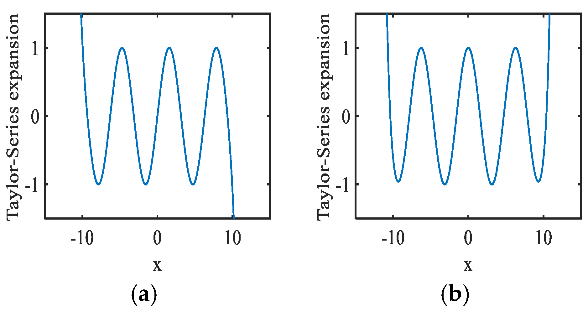
Figure 2.
IEEE-754 single-precision floating-point format.
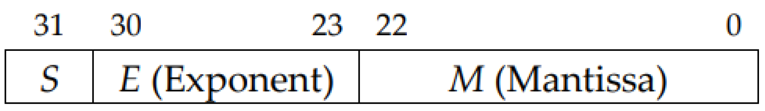

Table 1.
Scheme without mantissa division.
| Number | Mantissa Region | Center value a |
|---|---|---|
| R1-1 | M = 1.xxxxxx (1.0 ≤ M < 2.0) | 1.5 |
Table 2.
2-region division scheme.
| Number | Mantissa Region | Center value a |
|---|---|---|
| R2-1 | M = 1.0xxxxx… (1.0 ≤ M < 1.5) | 1.25 |
| R2-2 | M = 1.1xxxxx… (1.5 ≤ M < 2.0) | 1.75 |
Table 3.
4-region division scheme.
| Number | Mantissa Region | Center value a |
|---|---|---|
| R4-1 | M = 1.00xxxxx… (1.00 ≤ M < 1.25) | 1.125 |
| R4-2 | M = 1.01xxxxx… (1.25 ≤ M < 1.50) | 1.375 |
| R4-3 | M = 1.10xxxxx… (1.50 ≤ M < 1.75) | 1.625 |
| R4-4 | M = 1.11xxxxx… (1.75 ≤ M < 2.00) | 1.875 |
Table 4.
8-region division scheme.
| Number | Mantissa Region | Center value a |
|---|---|---|
| R8-1 | M = 1.000xxxx… (1.000 ≤ M < 1.125) | 1.0625 |
| R8-2 | M = 1.001xxxx… (1.125 ≤ M < 1.250) | 1.1875 |
| R8-3 | M = 1.010xxxx… (1.250 ≤ M < 1.375) | 1.3125 |
| R8-4 | M = 1.011xxxx… (1.375 ≤ M < 1.500) | 1.4375 |
| R8-5 | M = 1.100xxxx… (1.500 ≤ M < 1.625) | 1.5625 |
| R8-6 | M = 1.101xxxx… (1.625 ≤ M < 1.750) | 1.6875 |
| R8-7 | M = 1.110xxxx… (1.750 ≤ M < 1.875) | 1.8125 |
| R8-8 | M = 1.111xxxx… (1.875 ≤ M < 2.000) | 1.9375 |
| Accuracy |
||||||
|---|---|---|---|---|---|---|
| Taylor-series Expansion Region |
||||||
| R1-1 | 6 | 11 | 13 | 16 | 21 | |
Table 6.
Number of Taylor-series expansion terms that meets setting accuracy when the region of 1 ≤ x < 2 is divided by 2.
Table 6.
Number of Taylor-series expansion terms that meets setting accuracy when the region of 1 ≤ x < 2 is divided by 2.
| Accuracy |
||||||
| Taylor-series Expansion Region |
||||||
| R2-1 | 4 | 7 | 9 | 11 | 14 | |
| R2-2 | 3 | 6 | 8 | 9 | 12 | |
Table 7.
Number of Taylor-series expansion terms that meets setting accuracy when the region of 1 ≤ x < 2 is divided by 4.
Table 7.
Number of Taylor-series expansion terms that meets setting accuracy when the region of 1 ≤ x < 2 is divided by 4.
| Accuracy |
||||||
|---|---|---|---|---|---|---|
| Taylor-series Expansion Region |
||||||
| R4-1 | 3 | 6 | 7 | 8 | 11 | |
| R4-2 | 3 | 5 | 6 | 7 | 10 | |
| R4-3 | 3 | 5 | 6 | 7 | 9 | |
| R4-4 | 3 | 5 | 6 | 7 | 9 | |
Table 8.
Number of Taylor-series expansion terms that meets setting accuracy when the region of 1 ≤ x < 2 is divided by 8.
Table 8.
Number of Taylor-series expansion terms that meets setting accuracy when the region of 1 ≤ x < 2 is divided by 8.
| Accuracy |
||||||
|---|---|---|---|---|---|---|
| Taylor-series Expansion Region |
||||||
| R8-1 | 2 | 4 | 5 | 6 | 8 | |
| R8-2 | 2 | 4 | 5 | 6 | 8 | |
| R8-3 | 2 | 4 | 5 | 6 | 8 | |
| R8-4 | 2 | 4 | 5 | 6 | 8 | |
| R8-5 | 2 | 4 | 5 | 6 | 7 | |
| R8-6 | 2 | 4 | 5 | 6 | 7 | |
| R8-7 | 2 | 4 | 5 | 5 | 7 | |
| R8-8 | 2 | 4 | 5 | 5 | 7 | |
Table 9.
Required numbers of multiplications and additions/subtractions for n-term Taylor series expansion.
Table 9.
Required numbers of multiplications and additions/subtractions for n-term Taylor series expansion.
| # of Taylor-series expansion terms | # of multiplications | # of additions and subtractions |
|---|---|---|
| 3 | 3 | 3 |
| 4 | 4 | 4 |
| 5 | 4 | 4 |
| 6 | 5 | 5 |
| 7 | 5 | 5 |
| 8 | 6 | 6 |
Table 10.
LUT memory for region division by 4.
| Address () | LUT data |
| 00 | Reciprocal of a = 1.125 |
| 01 | Reciprocal of a = 1.357 |
| 10 | Reciprocal of a = 1.625 |
| 11 | Reciprocal of a = 1.875 |
Table 11.
Number of Taylor-series expansion terms that meets setting accuracy for one region of 1 ≤ x < 2.
Table 11.
Number of Taylor-series expansion terms that meets setting accuracy for one region of 1 ≤ x < 2.
| Accuracy |
||||||
|---|---|---|---|---|---|---|
| Taylor-series Expansion Region |
||||||
| R1-1 | 5 | 9 | 12 | 14 | 19 | |
Table 12.
Number of Taylor-series expansion terms that meets setting accuracy when the region of 1 ≤ x < 2 is divided by 2.
Table 12.
Number of Taylor-series expansion terms that meets setting accuracy when the region of 1 ≤ x < 2 is divided by 2.
| Accuracy |
||||||
|---|---|---|---|---|---|---|
| Taylor-series Expansion Region |
||||||
| R2-1 | 3 | 7 | 8 | 10 | 13 | |
| R2-2 | 3 | 6 | 7 | 8 | 9 | |
Table 13.
Number of Taylor-series expansion terms that meets setting accuracy when the region of 1 ≤ x < 2 is divided by 4.
Table 13.
Number of Taylor-series expansion terms that meets setting accuracy when the region of 1 ≤ x < 2 is divided by 4.
| Accuracy |
||||||
|---|---|---|---|---|---|---|
| Taylor-series Expansion Region |
||||||
| R4-1 | 3 | 5 | 6 | 7 | 10 | |
| R4-2 | 2 | 5 | 6 | 7 | 9 | |
| R4-3 | 2 | 4 | 5 | 6 | 8 | |
| R4-4 | 2 | 4 | 5 | 6 | 8 | |
Table 14.
Number of Taylor-series expansion terms that meets setting accuracy when the region of 1 ≤ x < 2 is divided by 8.
Table 14.
Number of Taylor-series expansion terms that meets setting accuracy when the region of 1 ≤ x < 2 is divided by 8.
| Accuracy |
||||||
|---|---|---|---|---|---|---|
| Taylor-series Expansion Region |
||||||
| R8-1 | 2 | 4 | 5 | 6 | 8 | |
| R8-2 | 2 | 4 | 5 | 6 | 7 | |
| R8-3 | 2 | 4 | 5 | 6 | 7 | |
| R8-4 | 2 | 4 | 5 | 5 | 7 | |
| R8-5 | 2 | 4 | 4 | 5 | 7 | |
| R8-6 | 2 | 4 | 4 | 5 | 7 | |
| R8-7 | 2 | 3 | 4 | 5 | 7 | |
| R8-8 | 2 | 3 | 4 | 5 | 7 | |
Table 15.
Required numbers of multiplications and additions/subtractions for N-term Taylor-series expansion.
Table 15.
Required numbers of multiplications and additions/subtractions for N-term Taylor-series expansion.
| # of Taylor-series expansion terms | # of multiplications | # of additions and subtractions | # of LUT words for N regions |
|---|---|---|---|
| 3 | 3 | 3 | 8N |
| 4 | 4 | 4 | 10N |
| 5 | 4 | 4 | 12N |
| 6 | 5 | 5 | 14N |
| 7 | 5 | 5 | 16N |
| 8 | 6 | 6 | 18N |
Table 16.
LUT memory for 4 regions (10 x 4 = 40 words).
| ) | LUT data |
|---|---|
| 00 |
for a = 1.125 |
| 01 |
for a = 1.357 |
| 10 |
for a = 1.625 |
| 11 |
for a = 1.875 |
Table 17.
The number of Taylor expansion terms required to meet the specified accuracy in the region .
Table 17.
The number of Taylor expansion terms required to meet the specified accuracy in the region .
| Accuracy |
||||||
|---|---|---|---|---|---|---|
| Taylor-series Expansion Region |
||||||
| R1-1 | 3 | 7 | 9 | 12 | 15 | |
Table 18.
Region is divided into 2 subregions, and the number of Taylor expansion terms required to meet the specified accuracy determined in each region.
Table 18.
Region is divided into 2 subregions, and the number of Taylor expansion terms required to meet the specified accuracy determined in each region.
| Accuracy |
||||||
|---|---|---|---|---|---|---|
| Taylor-series Expansion Region |
||||||
| R2-1 | 3 | 5 | 7 | 8 | 11 | |
| R2-2 | 2 | 5 | 6 | 7 | 10 | |
Table 19.
Region is divided into 4 subregions, and the number of Taylor expansion terms required to meet the specified accuracy determined in each region.
Table 19.
Region is divided into 4 subregions, and the number of Taylor expansion terms required to meet the specified accuracy determined in each region.
| Accuracy |
||||||
|---|---|---|---|---|---|---|
| Taylor-series Expansion Region |
||||||
| R4-1 | 2 | 4 | 5 | 6 | 9 | |
| R4-2 | 2 | 4 | 5 | 6 | 8 | |
| R4-3 | 2 | 4 | 5 | 6 | 8 | |
| R4-4 | 2 | 4 | 5 | 5 | 7 | |
Table 20.
Region is divided into 8 subregions, and the number of Taylor expansion terms required to meet the specified accuracy determined in each region.
Table 20.
Region is divided into 8 subregions, and the number of Taylor expansion terms required to meet the specified accuracy determined in each region.
| Accuracy |
||||||
|---|---|---|---|---|---|---|
| Taylor-series Expansion Region |
||||||
| R8-1 | 2 | 3 | 4 | 5 | 7 | |
| R8-2 | 2 | 3 | 4 | 5 | 7 | |
| R8-3 | 2 | 3 | 4 | 5 | 7 | |
| R8-4 | 2 | 3 | 4 | 5 | 6 | |
| R8-5 | 2 | 3 | 4 | 5 | 6 | |
| R8-6 | 2 | 3 | 4 | 5 | 6 | |
| R8-7 | 2 | 3 | 4 | 4 | 6 | |
| R8-8 | 2 | 3 | 4 | 4 | 6 | |
Table 21.
Relationship between arithmetic operations and Taylor series expansion terms.
| # of Taylor-series expansion terms | # of multiplications | # of additions and subtractions |
|---|---|---|
| 3 | 3 | 3 |
| 4 | 4 | 4 |
| 5 | 5 | 5 |
| 6 | 6 | 6 |
| 7 | 7 | 7 |
| 8 | 8 | 8 |
Table 22.
LUT memory with 4 regions.
| ) | LUT data |
|---|---|
| 00 |
for a = 1.125 |
| 01 |
for a = 1.357 |
| 10 |
for a = 1.625 |
| 11 |
for a = 1.875 |
Table 23.
Accuracy and required number of Taylor series terms in the region 1 ≤ x < 2.
| Accuracy |
||||||
|---|---|---|---|---|---|---|
| Taylor-series Expansion Region |
||||||
| R1-1 | 4 | 7 | 8 | 9 | 11 | |
Table 24.
Number of Taylor-series expansion terms that meets setting accuracy when the region of 1≤x<2 is divided by 2.
Table 24.
Number of Taylor-series expansion terms that meets setting accuracy when the region of 1≤x<2 is divided by 2.
| Accuracy |
||||||
|---|---|---|---|---|---|---|
| Taylor-series Expansion Region |
||||||
| R2-1 | 3 | 5 | 6 | 7 | 9 | |
| R2-2 | 3 | 5 | 6 | 7 | 9 | |
Table 25.
Number of Taylor-series expansion terms that meets setting accuracy when the region of 1≤x<2 is divided by 4.
Table 25.
Number of Taylor-series expansion terms that meets setting accuracy when the region of 1≤x<2 is divided by 4.
| Accuracy |
||||||
|---|---|---|---|---|---|---|
| Taylor-series Expansion Region |
||||||
| R4-1 | 3 | 4 | 5 | 5 | 7 | |
| R4-2 | 3 | 4 | 5 | 5 | 7 | |
| R4-3 | 3 | 4 | 5 | 5 | 7 | |
| R4-4 | 3 | 4 | 5 | 5 | 7 | |
Table 26.
Numbers of additions, subtractions and multiplications required for the n-term expansion.
| # of Taylor-series expansion terms | # of multiplications | # of additions and subtractions |
|---|---|---|
| 3 | 3 | 3 |
| 4 | 4 | 4 |
| 5 | 5 | 5 |
| 6 | 6 | 6 |
| 7 | 7 | 7 |
| 8 | 8 | 8 |
Table 27.
LUT memory with 4 regions.
| (αβ) | LUT data |
|---|---|
| 00 | Exp(a) for a = 1.125 |
| 01 | Exp(a) for a = 1.357 |
| 10 | Exp(a) for a = 1.625 |
| 11 | Exp(a) for a = 1.875 |
Table 28.
Number of Taylor-Series expansion terms to meet specified accuracy for one region of .
| Accuracy |
||||||
|---|---|---|---|---|---|---|
| Taylor-series Expansion Region |
||||||
| R1-1 | 13 | 15 | 18 | 22 | 23 | |
Table 29.
Number of Taylor-Series expansion terms to meet specified accuracy when the region of is divided by 2.
Table 29.
Number of Taylor-Series expansion terms to meet specified accuracy when the region of is divided by 2.
| Accuracy |
||||||
|---|---|---|---|---|---|---|
| Taylor-series Expansion Region |
||||||
| R2-1 | 10 | 11 | 13 | 16 | 16 | |
| R2-2 | 4 | 5 | 7 | 9 | 10 | |
Table 30.
Number of Taylor-Series expansion terms to meet specified accuracy when the region of is divided by 4.
Table 30.
Number of Taylor-Series expansion terms to meet specified accuracy when the region of is divided by 4.
| Accuracy |
||||||
|---|---|---|---|---|---|---|
| Taylor-series Expansion Region |
||||||
| R4-1 | 8 | 8 | 10 | 12 | 12 | |
| R4-2 | 4 | 5 | 6 | 8 | 8 | |
| R4-3 | 4 | 4 | 6 | 7 | 8 | |
| R4-4 | 4 | 4 | 5 | 7 | 7 | |
Table 31.
Required numbers of multiplications and additions/subtractions for n-term Taylor-series expansion.
Table 31.
Required numbers of multiplications and additions/subtractions for n-term Taylor-series expansion.
| # of Taylor-series expansion terms | # of multiplications | # of additions and subtractions |
|---|---|---|
| 3 | 3 | 3 |
| 4 | 4 | 4 |
| 5 | 5 | 5 |
| 6 | 6 | 6 |
| 7 | 7 | 7 |
| 8 | 8 | 8 |
Table 32.
LUT memory for 4 regions.
| (αβ) | LUT data |
|---|---|
| 00 |
for a = 1.125 |
| 01 |
for a = 1.357 |
| 10 |
for a = 1.625 |
| 11 |
for a = 1.875 |
Disclaimer/Publisher’s Note: The statements, opinions and data contained in all publications are solely those of the individual author(s) and contributor(s) and not of MDPI and/or the editor(s). MDPI and/or the editor(s) disclaim responsibility for any injury to people or property resulting from any ideas, methods, instructions or products referred to in the content. |
© 2026 by the authors. Licensee MDPI, Basel, Switzerland. This article is an open access article distributed under the terms and conditions of the Creative Commons Attribution (CC BY) license (http://creativecommons.org/licenses/by/4.0/).
Copyright: This open access article is published under a Creative Commons CC BY 4.0 license, which permit the free download, distribution, and reuse, provided that the author and preprint are cited in any reuse.


