
Submitted:
01 January 2026
Posted:
05 January 2026
You are already at the latest version
Abstract
The Wallonia region of Belgium aims to transition to a modern hydrogen infrastructure. Since hydrogen is much lighter than natural gas, so it is important to understand its nature and behavior while transporting through pipelines. This research aims to observe the pressure loss in pipelines due to surface roughness with H2 and other singular losses to find a solution to minimize the amount of pressure loss that occurs during transportation. This study involves numerical methods and gas equation models to determine thse pres-sure loss. This analysis includes the properties of hydrogen gas, pipeline material used, friction factor, pipeline efficiency, and other relevant properties of hydrogen and the pipe-lines.
To address this challenge, this study integrates numerical fluid dynamics methods with structural modelling of pipeline walls. It accounts for long-term friction effects, erosion over several years, radial pressure gradients (mixing pressure drop), acceleration effects, and gravity influences, considering the non-ideal behavior of gaseous hydrogen (GH2).
Keywords:
hydrogen pipeline
; pressure losses
; pressure loss equation model
; material roughness
; friction factor
; Reynolds number
1. Introduction
Hydrogen is a key component of green transition. As a result, countries are investing in hydrogen-based solutions to accelerate the transition to a low-carbon economy. The importance of hydrogen as an energy source arises from its extraordinary potential to address the converging problems of energy security and environmental sustainability. Hydrogen is a lightweight and abundant element with important implications for transportation via pipelines as it has low molecular weight and high diffusivity, making it efficient for movement in pipeline systems. However, hydrogen presents challenges such as leakage and material embrittlement [1,2]. This work examines the importance of hydrogen as an energy carrier, its physical, chemical properties and numerical modelling of hydrogen flow in pipelines, recent advancements in flow experiments, existing challenges of utilizing pipelines for hydrogen gas flow, and solutions. Hydrogen transport encompasses various modes, such as pipelines, tank trucks, and chemical carriers like ammonia. The prominent mode of hydrogen storage is high pressure storage and transportation in compressed gas containers. Another effective transportation method is through pipelines [3]. This mode of transportation establishes continuous, high-volume and cost-effective transportation over long distances. In the practical world, one of the potential ways to transport hydrogen gas is through natural gas pipelines. One such example in the UK is Project H21, which utilized the existing natural gas pipeline infrastructure to transport hydrogen gas. Any pipeline network consists of chains of distribution networks, such as gathering, transmission, distribution, service lines, re-compression of H2 gas pressure using a compressor on transmission lines[4].
The focus of the current study is on transportation pipelines, which are used to transport hydrogen over long distance. In the process of hydrogen transmission, pressure loss is major factor that resists the amount of hydrogen transportation to minimize the effect of pressure drop, various factors must be considered including pipeline length, diameter, material surface roughness, friction factor, operating pressure value, volumetric flow rate and hydrogen gas properties. In addition, factors that causes pressure drop, such as leakage and safety valves, must also be considered because an unexplained drop is sign of hydrogen releases which could lead to explosion due to the hydrogen’s highly flammable character. To compute pressure loss accurately leakage and safety value has to been taken consideration that provides baseline if actual pressure is lower than the calculated pressure to avoid unexpected pressure drop.
In this study, the pressure drops in a transportation pipeline carrying hydrogen gas were calculated for a fixed high volumetric flow rate and a pipeline distance of 100 km to observe the pressure drop value for different operating pressure values ranging from 50 to 120 bar [3]. At this moment, no compression station is considered because the distance considered here is optimal, and also no elevation difference condition is considered.
2. Materials and Methods
Pipelines can be made from a wide range of materials that show relative contributions per distance by gas of various types. Carbon steel is the alloy in hydrogen gas transmission pipelines.
Steels used in hydrogen pipeline services should have a maximum hardness of approximately 22 HRC (Hardness Rockwell C) or 250 HB (Hardness Brinell). This hardness limit is approximately equivalent to a tensile strength limit of approximately 800MPa. Materials with low-strength steels is sometimes recommended for H2 pipelines. In this study, material API X52 and its properties were used, as it is the most widely used material in pipelines, and the pressure loss calculation was based on the same material roughness values [3,5].
The Figure 1 shows the transportation of hydrogen gas through pipeline. The flow of hydrogen gas is due to principle of pressure difference induced flow. The interaction between viscosity of gas and friction with pipe wall encounters the pressure drop. As velocity of gas inside pipeline increases the pressure drop will increases proportionally. To overcome larger pressure drop compression stations needs to installed at distance of 80-100km. The functionality of compressor station restores the pressure losses when hydrogen gas needs to travel long distances. During this action of hydrogen gas transport, maintaining the gas velocity with in the limit which is called as erosional limit is very important to avoid any catastrophic situation within the line of pipeline connections. This erosional velocity limit is shown in Figure 2 with respect to operating pressure of pipeline.
3. Method of Computing and Validation of Equation Model
To begin with, the computation of pressure drop involves many models available. In this study, the American Gas Association (AGA) model was used. This model was is that the equation has surface roughness and pipeline efficiency factors inside, which have a direct influence on pressure loss. The other models are named as follows.
- Panhandle A equation
- Panhandle B equation
- Weymouth equation
- General flow equation
To calculate the pressure loss, the AGA (American Gas Association) equation is given by the numerical equation [6].
Q - Flow rate of gas at standard conditions(m3/s)
Ts - Base H2 Temperature (K)
Ps - Base H2 Pressure (bar)
E - Pipeline efficiency (typically between 0.8-1)
1 in the absence of field data (also for a new straight pipe with no diameter change)
0.95 for very good operating conditions, typically through the first 12–18 months
0.92 for average operating conditions
0.85 for unfavorable operating conditions
d - Internal diameter of pipeline (m)
P1 – Inlet H2 pressure (bar)
P2 – Outlet H2 pressure (bar)
S - Specific gravity 0.0696 for H2 (dimensionless)
L - Length of pipeline (km)
Z - Compressibility factor of H2 gas (dimensionless)
- Absolute Surface Roughness of material (m)
- Relative density of flowing gas for hydrogen (0.0696)
Tavg - Average temperature of H2 gas (K)
The friction factor f was calculated using the Colebrook-White of equation (2):
f - Friction factor (dimensionless)
- Pipeline material roughness (m)
D - Internal diameter of pipeline (m)
Re - Reynolds number, which is calculated by equation (3):
- Reynolds Number (dimensionless)
ρ - Density of Hydrogen gas (0.083 kg/m3)
- Dynamic viscosity of H2 gas (8.76 x Pa.s)
Vmax - Velocity of hydrogen gas flow (m/s)
D - Diameter of pipeline (m)
V is the H2 gas velocity, calculated using the equation (4).
Pb - Base pressure (bar)
Tb - Base temperature in (K)
Z - Compressibility factor of H2 gas (dimensionless)
T - Flow temperature of hydrogen (K)
P - Inlet pressure (bar)
D - Diameter of pipeline (m)
Q - Gas volumetric flow rate (m3/s)
The pressure drop ∆p is calculated for a given flow rate Q in m3/s, a diameter of pipeline D, and a given length L of pipeline, the outlet pressure P2 is calculated by equation (5):
P2 - Pressure at outlet (bar)
- Pressure difference in (bar)
P1 - Pressure at inlet in (bar)
The erosional velocity represents the upper limit of the gas velocity in the pipeline. Higher velocities can cause pipe wall erosion over a time. In AGA, the erosional velocity Vmax is calculated by equation (6):
Vmax - Erosional velocity (m/s)
P - Gas pressure (bar)
T - Gas temperature (K)
Z is the compressibility factor of H2 gas (dimensionless)
R - Ideal gas constant (J/kg K)
Transmission factor F is considered to be the opposite of the friction factor f. Whereas the friction factor indicates the difficulty of moving a certain quantity of gas through a pipeline, the transmission factor is a direct measure of the amount of gas that can be transported through the pipeline. As the friction factor increases, the transmission factor decreases and therefore, the gas flow rate also decreases [7]. Conversely, the higher the transmission factor, the lower the friction factor, and therefore, the higher the flow.
F – Transmission factor (dimensionless)
– Friction factor (dimensionless)
In this study, gas was considered to flow from point 1 to point 2, and the pipeline shape was cylindrical. If P1=P2, there would be no driving force for gas to flow. The gas flow is primarily due to the pressure difference between the two points and partly due to the elevation difference (H2-H1). As the gas flows through the pipe, it encounters a drop in pressure owing to the friction between the flowing gas and pipe wall. It is therefore the reason that encounters that the higher the pipe roughness and length, the higher the pressure drop. There are additional losses, such as frictional losses due to elbows, branching and control valves. The velocity (V) of the gas, which is proportional to the volumetric flow rate (Q) [9], also changes depending on the cross-sectional area (A) of the pipe and the pressure and temperature of the gas.
Considering the elevation parameter, there can be two cases: first, pipeline without an elevation difference shown in Figure 3 and second, pipeline with an elevation difference, that is, a height difference between two segments of a pipeline Figure 4 . When the pipeline is assumed with an elevation difference, then an additional parameter comes into existence, that is, the elevation adjustment parameter and is dimensionless given by equation (6).
H1 and H2 - Inlet and outlet elevations (m).
s - elevation adjustment parameter (dimensionless).
Z- Compressibility factor (dimensionless)
Tf – Gas flow temperature in (K)
Considering the effect of elevation, the length of the pipeline is now addressed as an equivalent length, which is represented as equation (9):
With this L in equation (1), is replaced with Le , the equivalent pipe length in km.
A study on the influence of temperature was conducted. All real gases have an inversion temperature at which the Joule-Thompson coefficient changes its sign. At room temperature, this coefficient is positive for most gases, except for hydrogen, neon, and helium. The Joule-Thompson coefficientis 0.5 °K/bar for natural gas and -0.035 °K/bar for hydrogen. To establish the temperature effect, Equation [10,11] are used to determine the temperature values, and it is observed that there is no high spike increase in temperature.
Hydrogen behaves differently and has a Joule-Thomson coefficient μJT at 1 bar and 300K around -0.03 K/bar. The negative sign indicates that under these conditions, hydrogen is heated during expansion. The Joule-Thomson co-efficient for different gas temperature of hydrogen is shown in Figure 5. However, the low absolute value of the Joule-Thomson coefficient means that, in practice, the temperature increase of hydrogen will be quite small, apart from in the case of large pressure changes in a hydrogen refueling station.
The final temperature was calculated using the equation (11).
T2 - Final temperature (K)
T1 - Initial temperature (K)
P1 and P2 - Initial and final pressure (bar)
- Joule-Thomson coefficient (K/bar)
4. Simulation Setup
Computation Fluid Dynamics (CFD) software ANSYS Fluent 2022R1 version was used to perform the simulation in order to analyze the mathematehical model and CFD to make it scalable for CFD analysis the geometry of model was scaled to 100m in length and 0.1m in diameter as initial stage to analyze and understand the pressure loss phenomenon in a system [12,13]. Addition to this following parameters were considered (i) material API X52 and its properties [12] (ii) hydrogen gas properties (iii) prevent reverse flow during simulation (iv) material surface roughness 0.02mm.
As the flow was turbulent in the system k-ε turbulent model[14] was selected for the simulation of hydrogen gas in the X52 steel pipe material. The reason for this model is its importance and robustness, which makes it a stable and reliable starting point if CFD analysis. While the AGA equation focuses on pressure loss due to material surface roughness and friction factor the k-ε RANS model focuses on the work done by the fluid and solving the Navier-Stoke equation. The implementation of surface roughness in ANSYS Fluent was performed using wall functions with an equivalent roughness height to represent the overall effect on shear stress and turbulence. Roughness modifies the wall boundary condition through the roughness height ks in the wall function thereby increasing the shear stress that affects the amount of pressure loss. This is explained with the equation of state
Shear stress is function of friction factor
represents dimensionless roughness height with an increase in the roughness height ks the increases which results an increase in pressure loss.
3.1. Meshing
Figure 6 represents mesh performed, and a generated total of 2396841 elements were created with a mesh element size of 5mm to build the geometry. In addition an inflation layer was applied to refine the near-wall regions of the mesh a total of 5 layers were added. An inside visualisation mesh inspection was made on model to check the mesh quality as shown in Figure 7.
5. Results
In this study, two extreme conditions were considered: when a pipeline with an internal diameter of 1m is in a new condition with a material roughness of APIX52 is of 0.02mm, and when the pipeline is severely corroded with the same material, increasing its roughness to 1.5mm due to more usage over the period. The related pressure losses were computed using the same volumetric flow rate of 100m3/s, and the distance considered was 100km with no compression station in between and no elevation difference. An inlet pressure of 50bar was assumed because most of the existing natural gas pipelines are equipped to operate at approximately 50-120 bar at 100m3/s volumetric flow rate. All units used in this calculation are SI units.
Using the AGA equation, a numerical computation was performed using the Python tool. The results were observed for a distance of 100km. With the lowest initial pressure of 50 bar and the highest initial pressure of 120 bar for 0.02mm material roughness, the pressure losses obtained were 29.92 bar and 9.08 bar, respectively, and the gas velocity at the outlet was 77.25m/s and 13.98m/s respectively. With the same conditions, when material roughness is 1.5mm, the pressure losses are 60.66 bar for the lowest initial pressure of 72 bar and 23.34 bar for the highest initial pressure of 120 bar, with outlet velocity found to be 136m/s and 16.04m/s, respectively. It is also observed that as the roughness increases, the initial pressure also increases to make the gas flow through the pipelines. Table 1 shows the pressure loss computed for an initial pressure of 50 to 120 bar and graphical representation is shown in Figure 8. The corresponding gas velocity in comparison with actual velocity for surface roughness 0.02mm is shown in Figure 9. The relation between fricition factor and Reynolds number for 0.02mm is shown in Figure 10. As the roughness of the material increases, the initial pressure should be increased. The reason to increase the initial pressure is that the pipeline system is not in a condition to accept the pressure values that are used when the pipeline is in good condition with low roughness. Table 2 shows the pressure loss when the surface roughness is 1.5mm The pressure loss when roughness is 1.5mm is shown in Figure 11. The corresponding gas velocity in comparison with actual velocity for surface roughness 1.5mm is shown in Figure 12. The relation between fricition factor and Reynolds number for 0.02mm is shown in Figure 13.
In this work it is also observed the relation between friction factor and Reynolds number that establishes the inversely propotional relation. The fricition factor is higher for lower Reynolds number and lower for higher Reynolds number. The physics behind this nature is when the flow is turbulant for lower Reynolds number viscous effect are still significant this causes higher wall shear stress that inturn makes friciton factor higher. The effect of surface roughness on fricition factor and Reynolds number for different roughness values is shown in Figure 14.
The CFD model k- ε model was selected to establish a comparison between CFD and AGA model for surface roughness of 0.02mm. The comparison was made based on dP/dx area weight average was used for inlet and outlet region of CFD to compute pressure losses over length of 100m as shown in Figure 15 and the velocity profile of gas is shown in Figure 16. The AGA and CFD results were computed for 100m and close comparison of pressure loss and velocity of gas were made as shown in Table 5. Using this as a base reference calculations were made for 100km distance pipeline as shown in Table 6

Table 3.
Change in temperature of H2 gas for surface roughness of 0.02mm.
| Initial Pressure in bar | Final Pressure in bar | Initial temperature in K | Final Temperature in K | Percentage of temperature difference in% |
|---|---|---|---|---|
| 50 | 20.08 | 300 | 301.05 | 0.35 |
| 60 | 30.77 | 300 | 301.02 | 0.34 |
| 70 | 52.95 | 300 | 300.60 | 0.19 |
| 80 | 65.60 | 300 | 300.50 | 0.16 |
| 90 | 77.48 | 300 | 300.44 | 0.14 |
| 100 | 88.90 | 300 | 300.39 | 0.12 |
| 110 | 100.02 | 300 | 300.35 | 0.11 |
| 120 | 110.92 | 300 | 300.32 | 0.10 |
Table 4.
Change in temperature of H2 gas for the surface roughness of 1.5mm.
| Initial Pressure in bar | Final Pressure in bar | Initial temperature in K | Final Temperature in K | Percentage of temperature differ ence in% |
|---|---|---|---|---|
| 72.00 | 11.34 | 300 | 302.12 | 0.70 |
| 80.00 | 36.67 | 300 | 301.52 | 0.50 |
| 90.00 | 55.17 | 300 | 301.22 | 0.40 |
| 100.00 | 70.31 | 300 | 301.04 | 0.34 |
| 110.00 | 83.93 | 300 | 300.91 | 0.30 |
| 120.00 | 96.66 | 300 | 300.82 | 0.27 |
Table 5.
Comparison between AGA and CFD results for 100m pipe length (roughness = 0.02mm).
| Initial Pressure in bar | Velocity of H2 gas in m/s | Pressure Loss in bar | ||
|---|---|---|---|---|
| AGA | CFD | AGA | CFD | |
| 50 | 73.78 | 63.39 | 0.043 | 0.053 |
| 60 | 61.20 | 52.96 | 0.039 | 0.045 |
| 70 | 52.40 | 45.43 | 0.036 | 0.039 |
| 80 | 45.95 | 39.75 | 0.031 | 0.036 |
| 90 | 40.68 | 35.36 | 0.029 | 0.032 |
| 100 | 36.59 | 31.84 | 0.025 | 0.029 |
| 110 | 33.25 | 28.95 | 0.022 | 0.025 |
| 120 | 30.46 | 26.55 | 0.015 | 0.021 |
Table 6.
Comparison between AGA and CFD results for 100m pipe length (roughness = 0.02mm).
| Initial Pressure in bar | Velocity of H2 gas in m/s | Pressure Loss in bar | ||
|---|---|---|---|---|
| AGA | CFD | AGA | CFD | |
| 50 | 73.78 | 63.39 | 43.39 | 45.12 |
| 60 | 61.20 | 52.96 | 39.45 | 41.24 |
| 70 | 52.40 | 45.43 | 36.63 | 39.78 |
| 80 | 45.95 | 39.75 | 31.21 | 36.63 |
| 90 | 40.68 | 35.36 | 30.23 | 32.59 |
| 100 | 36.59 | 31.84 | 25.11 | 29.81 |
| 110 | 33.25 | 28.95 | 22.01 | 25.33 |
| 120 | 30.46 | 26.55 | 15.23 | 21.58 |
6. Conclusions
Determining basic thermodynamics parameters of transported gas as a function of pipeline length is helpful in the calculation of pressure drop. With H2 the pressure drop is high at low initial pressure values and low at high initial pressure values, which is due to the pretty much different velocity of gas that is travelling inside the pipeline. As the pipeline ages, the material roughness increases with time, due to which it is observed that the pressure losses are even higher, and it is not possible to start the gas at an initial pressure of 50 bar like when the pipeline is in new condition. The compression station has been excluded in this current analysis to quantify the pressure loss resulting from its absence.
In this present state of work two extreme cases of pipeline conditions have been used which are: when pipeline is in new condition and secondly when pipeline is severely corroded that impacts change of roughness of material. Further the work analyzes variations in volumetric flow rate to determine their impact on pressure loss and flow conditions within the pipeline.
The role of pipeline efficiency is seen as important. Pipeline efficiency is representation of pipeline operation conditions with the time of usage. Typical values are as follows: 0.8 for unfavorable operating conditions, 0.92 for average operating conditions, 0.95 for very good operating conditions, typically through first 12–18 months, 1 in the absence of field data (also for new straight pipe with no diameter change). Further computation involves different scenarios to compute and compare the pressure losses with different conditions that mainly involve the phases of pipeline that come in between the new pipeline and to severely corroded phase, the pipeline efficiency, change in volumetric flow rate, elevation differences, and pipeline distance.
The results presented in Table 6 provide the comparison between mathematical model results and CFD results provides validation for the choice of pipeline operating pressure at required velocity. The change in velocity has its significance on change in Reynolds number and friction factor which results in an amount of pressure losses. It is observed that the velocity of hydrogen gas must be maintained within the limit of erosional velocity as presented in Figure 2. In addition to this the material surface roughness has a very important role that determines the friction factor that influences the pressure loss. During the analysis it was observed that pressure losses were significantly higher for pipes with smaller diameter and lower pressure losses for larger diameter due to effect of the surface-to-volume ratio of pipe.
In conclusion, the selection of pipeline material is critical, particularly regarding specific properties such as surface roughness that has direct influence on the pressure loss to overcome this regular maintenance of pipelines must be followed with the application of a material coating on the internal surface of pipes which is one of the method to maintain roughness of material. As the rate of surface roughness increases the pressure losses in pipeline also increase. We must maintain the material surface roughness within the limit before it reaches higher values in order to keep minimal pressure losses in pipelines.
Author Contributions
Conceptualization, AB.; methodology AB..; validation AB.; formal analysis, AB and PH.; investigation, AB.; resources, AB.; data curation, AB.; writing—original draft preparation, AB.; writing—review and editing, AB,PH ; visualization, AB.; supervision, PH and JPP.; project administration, PH and JPP.; funding acquisition, PH. All authors have read and agreed to the published version of the manuscript
Funding
This work is supported by SPW Economy Employment Research of the Walloon Region and the Walloon Region Recovery Plan, within the framework of the agreement no. 2310142
Data Availability Statement
The original contributions presented in this study are included in the article. Further inquiries can be directed to the corresponding author.
Acknowledgments
The author gratefully acknowledges the Win4Excellence project “TiNTHyN”

Conflicts of Interest
The funders had no role in the design of the study; in the collection, analyses, or interpretation of data; in the writing of the manuscript; or in the decision to publish the results.
Abbreviations
The following abbreviations are used in this manuscript:
| AGA | American Gas Association |
| JT | Joule – Thompson |
| CFD | Computational Fluid Dynamics |
References
- Kuczynski, Szymon; Łaciak, Mariusz; Olijnyk, Andrzej; Szurlej, Adam; Włodek, Tomasz. Thermodynamic and Technical Issues of Hydrogen and Methane-Hydrogen Mixtures Pipeline Transmission. Energies 2019, 12, 569. [Google Scholar] [CrossRef]
- Haeseldonckx, Dries; D’haeseller, William. The Use of The Natural-Gas Pipeline Infrastructure for Hydrogen Transport in A Changing Market Structure. International Journal of Energy 2007, Vol. 32(Issues 10-11), Pages 1381–1386. [Google Scholar] [CrossRef]
- Khan, M.A.; Young, C.; Layzell, D.B. The Techno-Economics of Hydrogen Pipelines. Transition Accelerator Technical Briefs 2021, Vol. 1(Issue 2), Pg. 1–40. [Google Scholar]
- Jottrand, Samuel; Hendrick, Patrick. Centrifugal Compressor Preiminary Design Optimization for a Hydrogen Pipeline Compression Station. ASME Turbo Expo 2024 2024, GT2024–123827. [Google Scholar] [CrossRef]
- Hydrogen Pipeline Systems Igc Doc 121/14 Revision of Doc 121/04. European Industrial Gases Association AISBL.
- American Gas Association (AGA) equation for fully turbulent isothermal gas flow (Reference: Eq-17-18, Section 17, GPSA Engineering Data Book, Eleventh Edition. 1998.
- Menon, E.S. Gas Pipeline Hydraulics; ISBN 0-8493-2785-7.
- Włodek, Tomasz; Łaciak, Mariusz; Kurowska, Katarzyna; Węgrzyn, Łukasz. AGH Drilling Oil Gas 2016, 33. [CrossRef]
- Abbas, Abubakar Jibrin; Hassani, Hossein; Burby, Martin; John, Idoko Job; ORCID. An Investigation into the Volumetric Flow Rate Requirement of Hydrogen Transportation in Existing Natural Gas Pipelines and Its Safety Implications. International Journal of Hydrogen Energy 2024, 67, 136–149. [Google Scholar] [CrossRef]
- Haeseldonckx, Dries. Concrete transition issues towards a fully-fledged use of hydrogen as an energy carrier. Ph.D. Report, KU Leuven, Belgium, August 2009. [Google Scholar]
- Raj, Aashna; Larsson, I.A. Sofia; Ljung, Anna-Lena; Forslund, Tobias; Andersson, Robin; Sundstrom, Joel; Lundstrom, T. Staffan. Evaluating hydrogen gas transport in pipelines: Current state of numerical and experimental methodologies. International Journal of Hydrogen Energy 2024, 67, 136–14. [Google Scholar] [CrossRef]
- Kurz, R; Lubomirsky, M; Bainier, F. Hydrogen in pipelines impact of hydrogen transport in natural gas pipelines. Paper No: GT2020-14040 2020, V009T21A001. [Google Scholar]
- Tan, Kun; Mahajan, Devinder; Venkatesh, T.A. Computational Fluid Dynamic Modeling of Methane-Hydrogen Mixture Transportation in Pipelines: Understanding the Effects of Pipe Roughness, Pipe Diameter and Pipe Bends. International journal of Hydrogen Energy 2024, Volume 49, Part-D, 1028–1042. [Google Scholar] [CrossRef]
- Anderson, John D, Jr. Computational Fluid Dynamics; ISBN 0-07-001685-2.
Figure 1.
Schematic representation of a hydrogen gas pipeline.
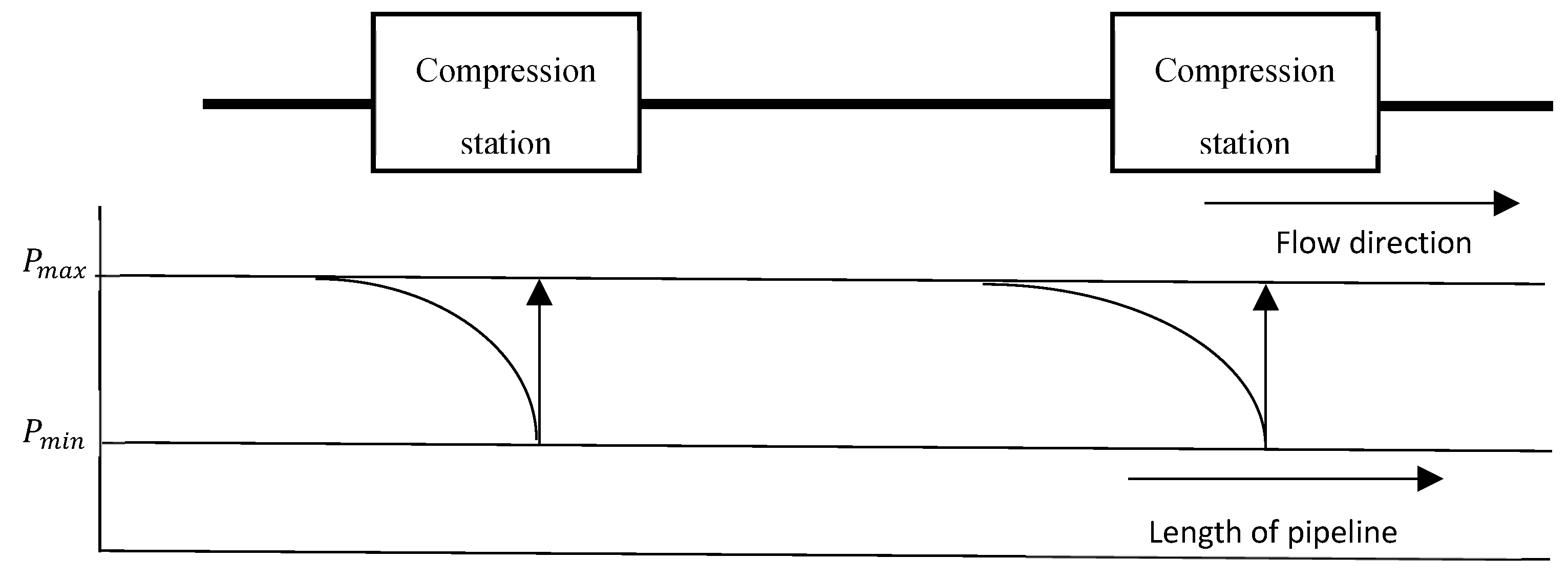
Figure 2.
Erosional velocity limit corresponding to H2 pressure.
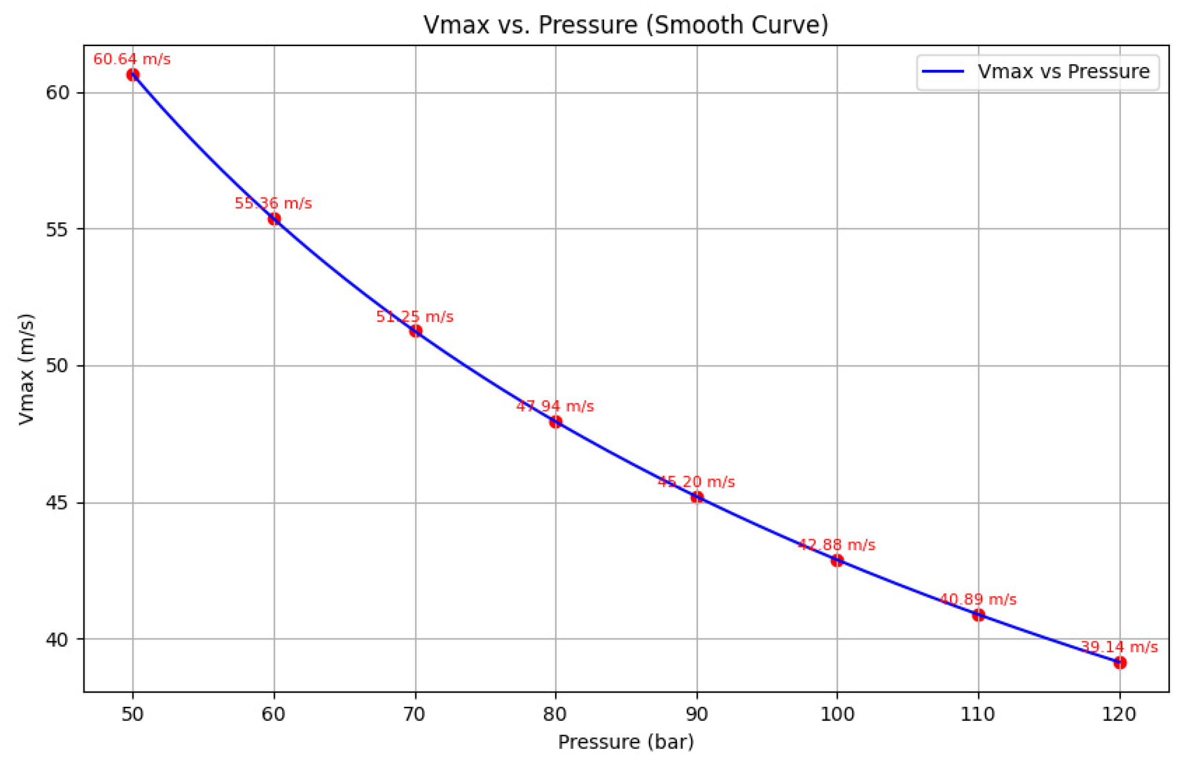
Figure 3.
Schematic representation of a GH2 pipeline with no elevation difference.
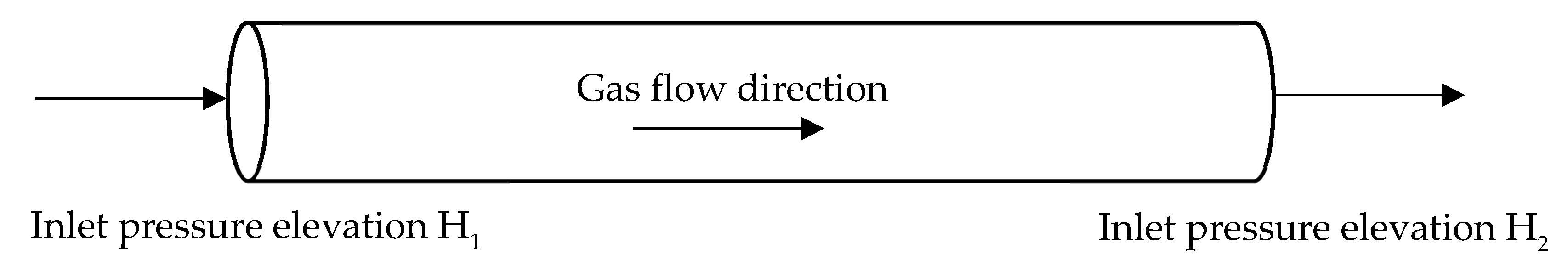
Figure 4.
Schematic representation of a GH2 pipeline with elevation difference.
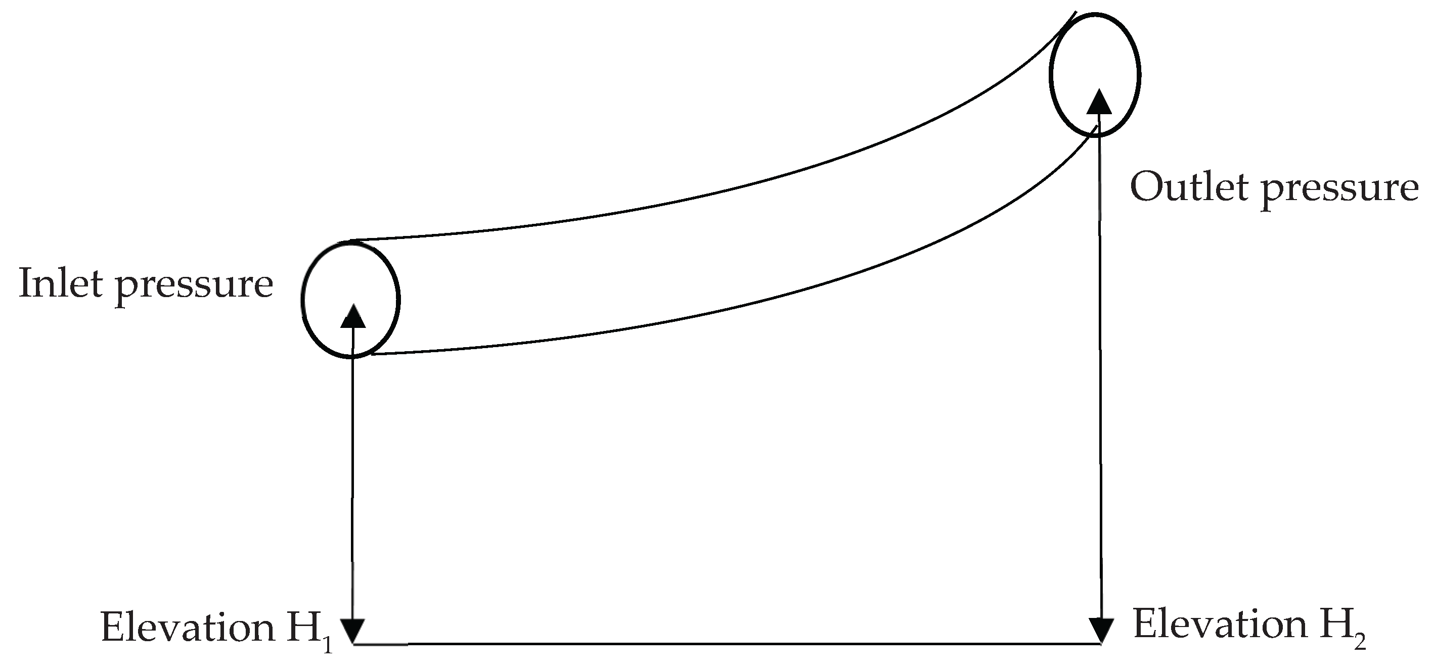
Figure 5.
Joule-Thompson co-efficient for hydrogen gas at different temperatures.
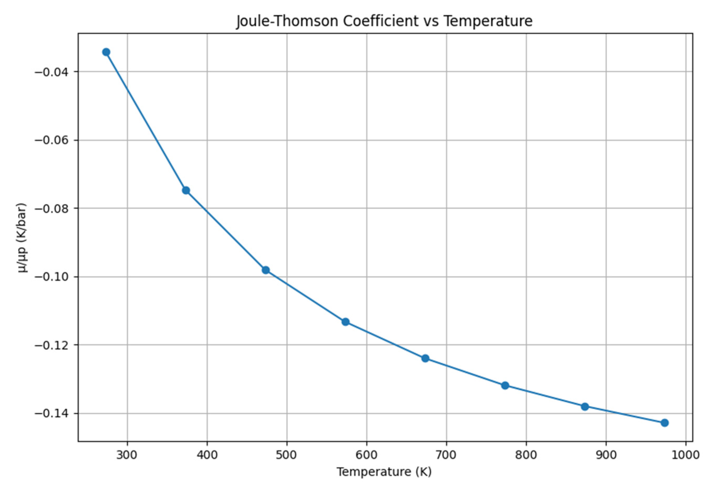
Figure 6.
Inflation layer on the model.
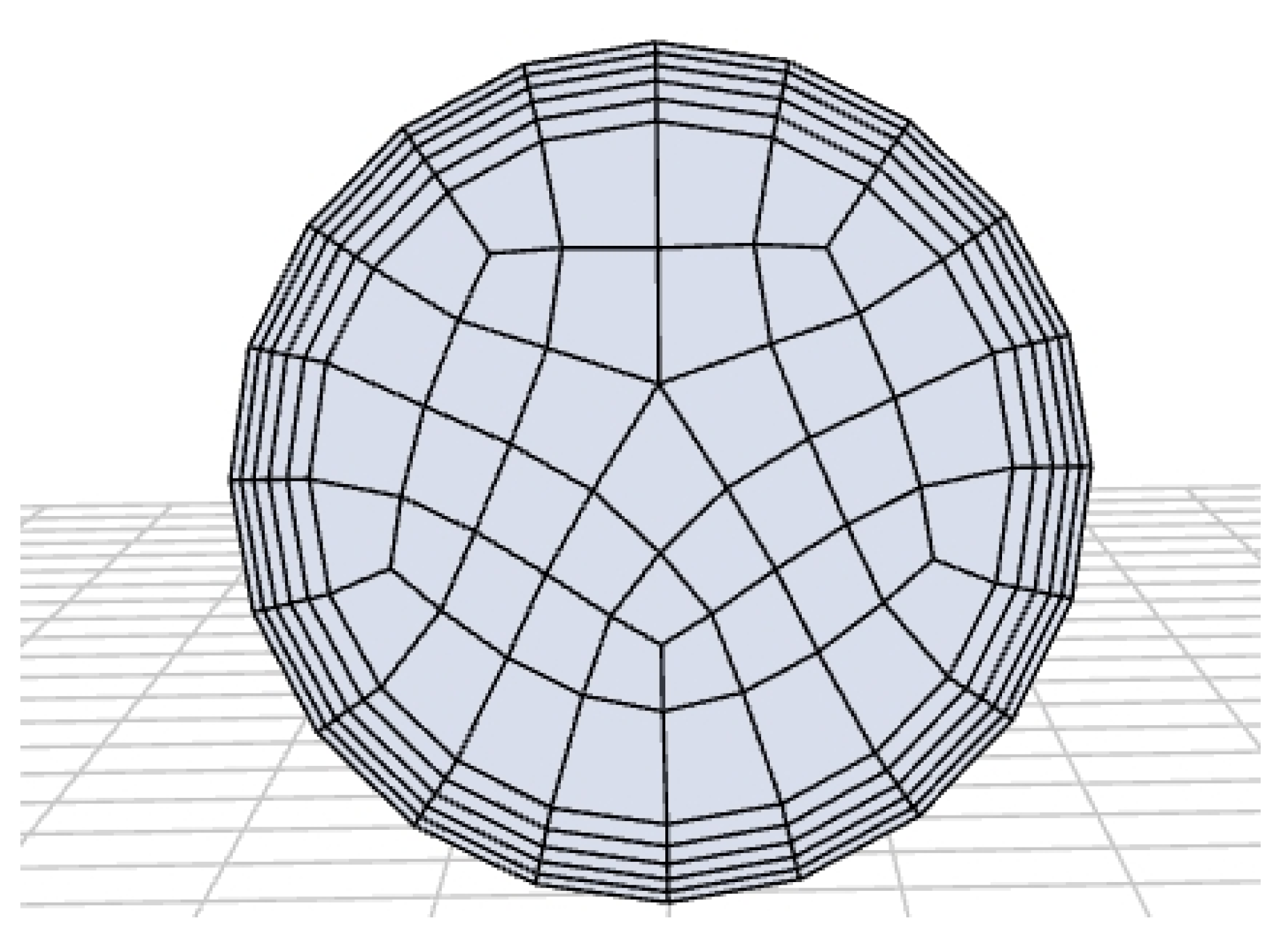
Figure 7.
Isometric mesh view inside a pipe.
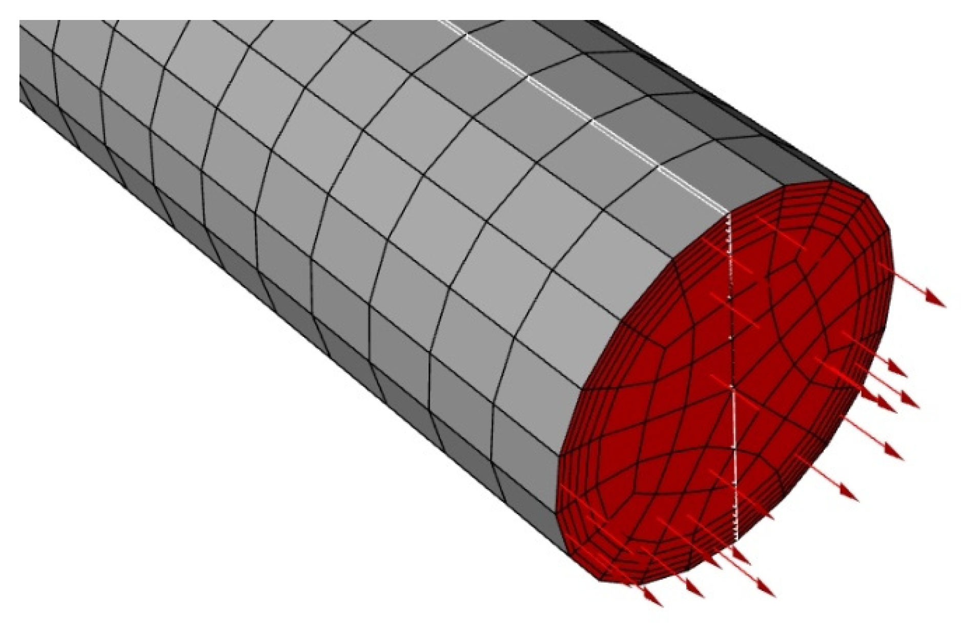
Figure 8.
Pressure loss vs initial pressure for surface roughness of 0.02mm.
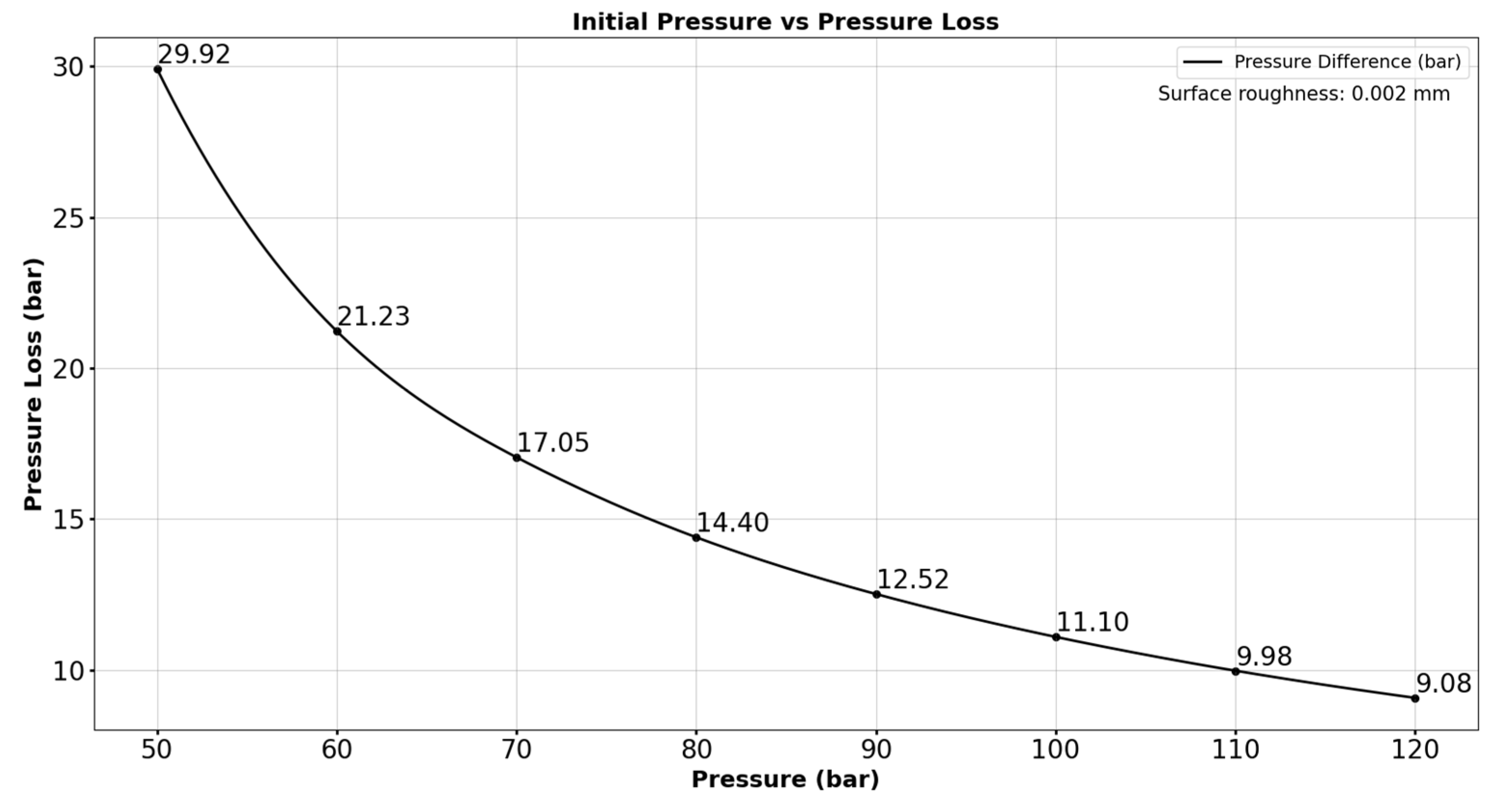
Figure 9.
Erosional velocity and actual velocity for a given gas pressure.
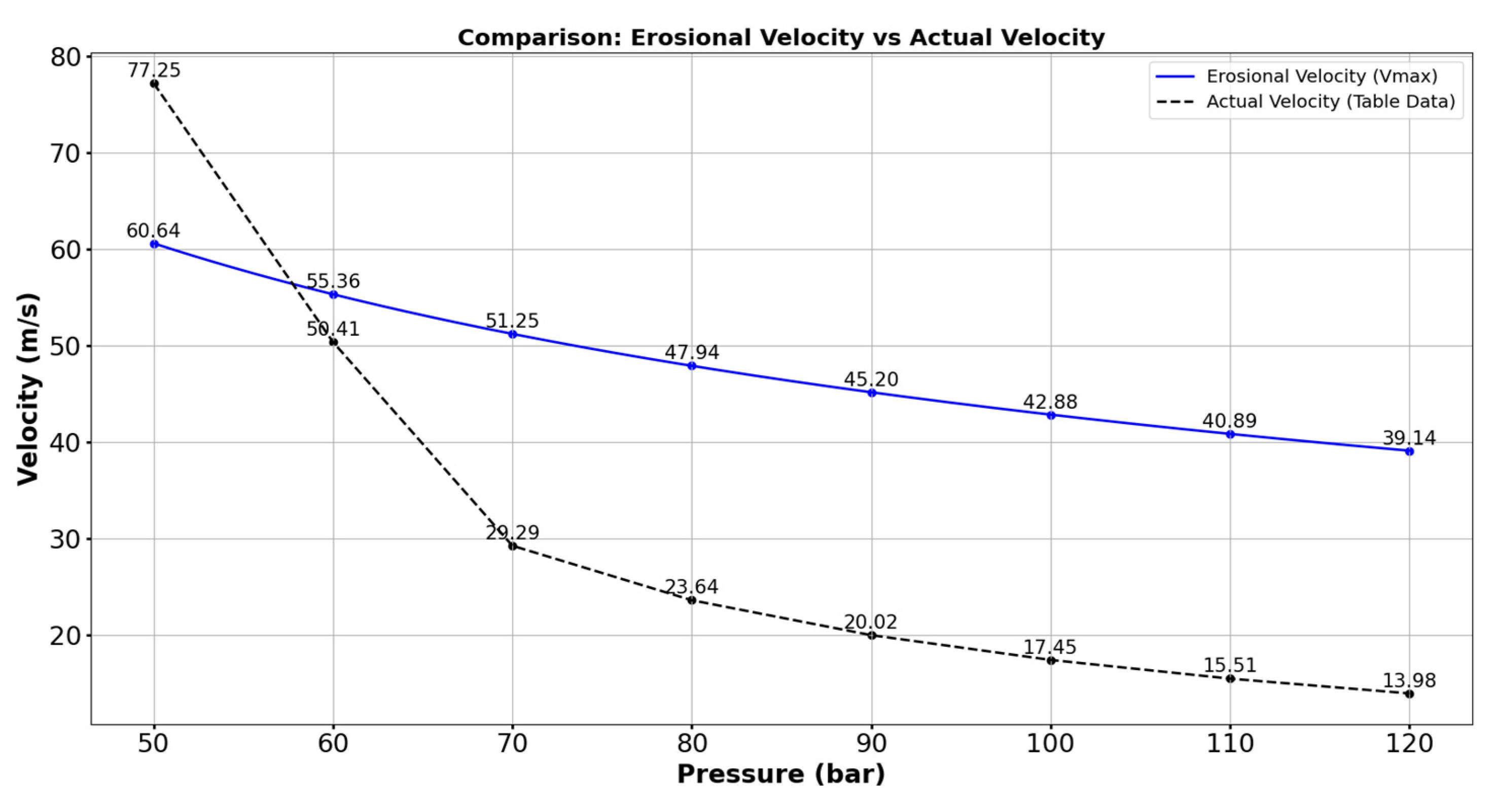
Figure 10.
Reynolds number and friction factor for surface roughness 0.02mm.
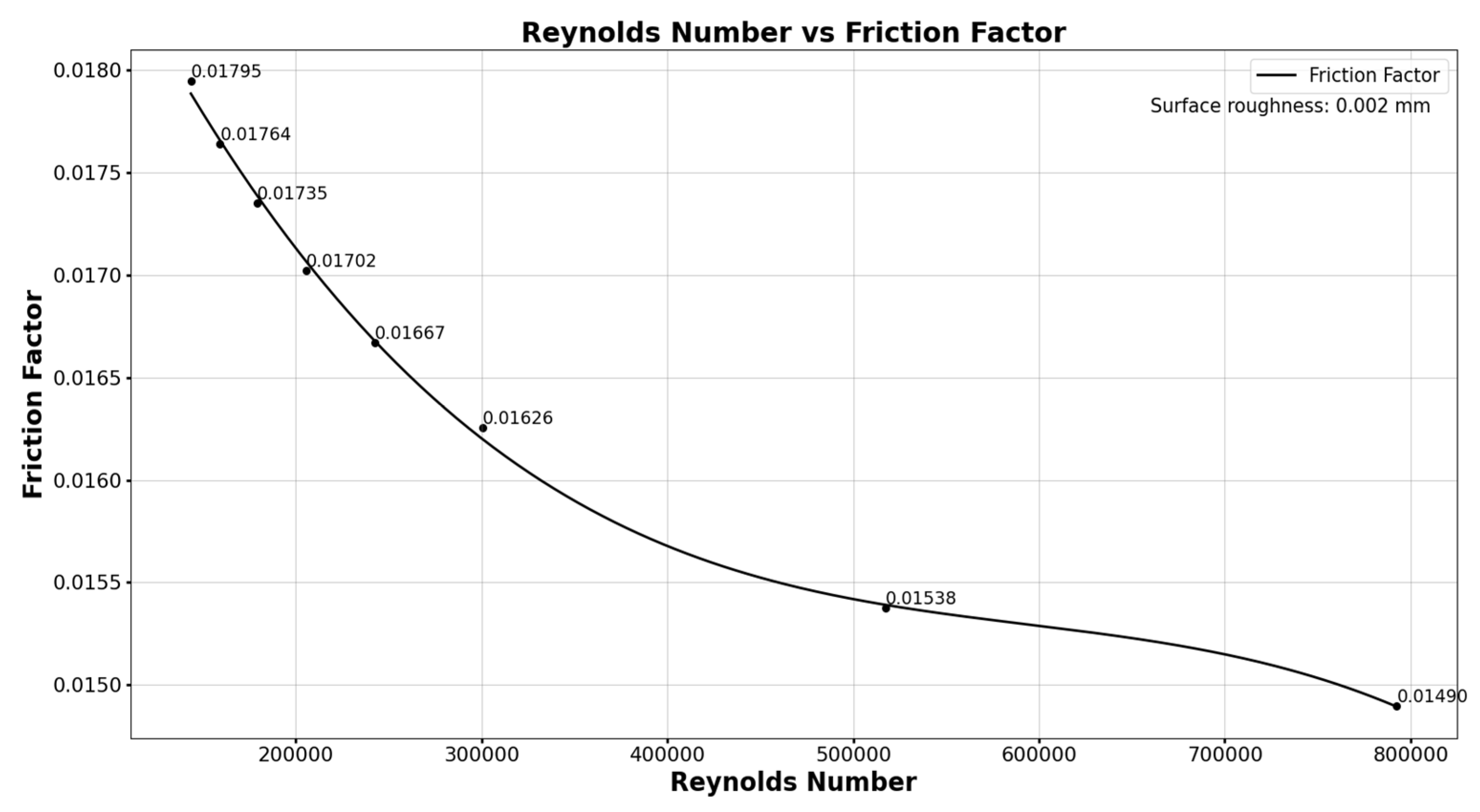
Figure 11.
Pressure loss vs initial pressure for surface roughness of 1.5mm.
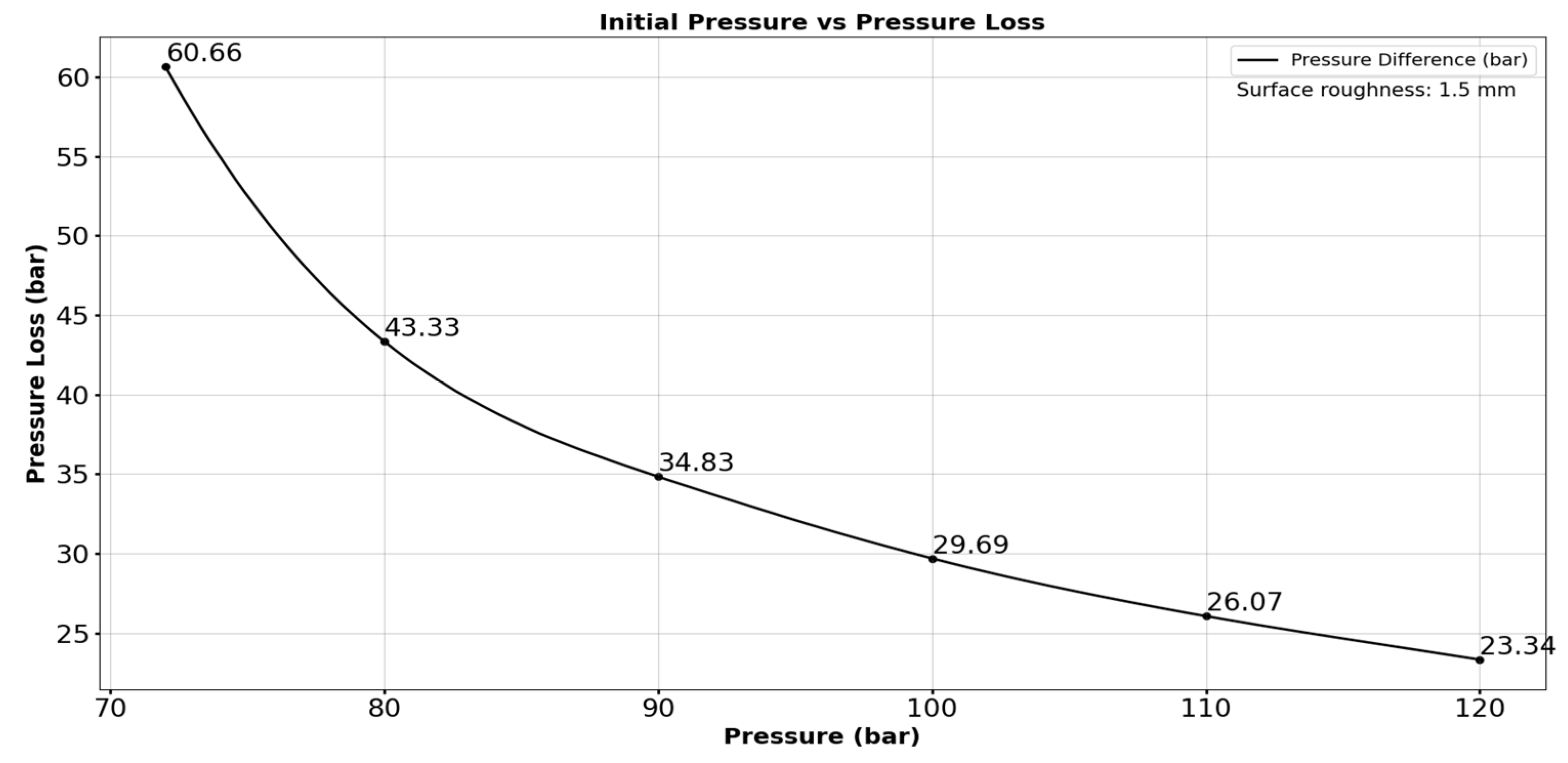
Figure 12.
Erosional velocity and actual velocity for given gas pressure.
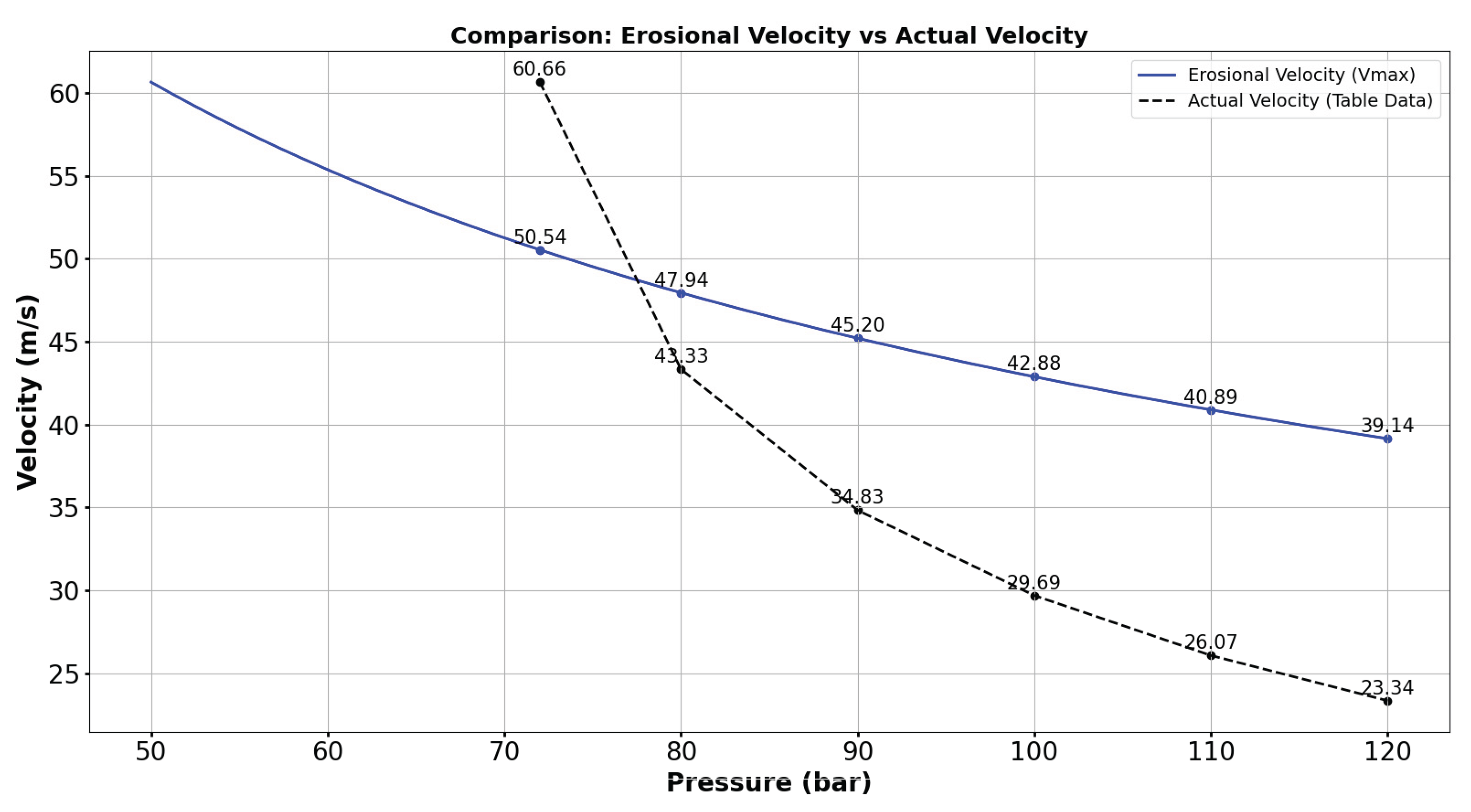
Figure 13.
Reynolds number and friction factor for surface roughness 1.5mm.
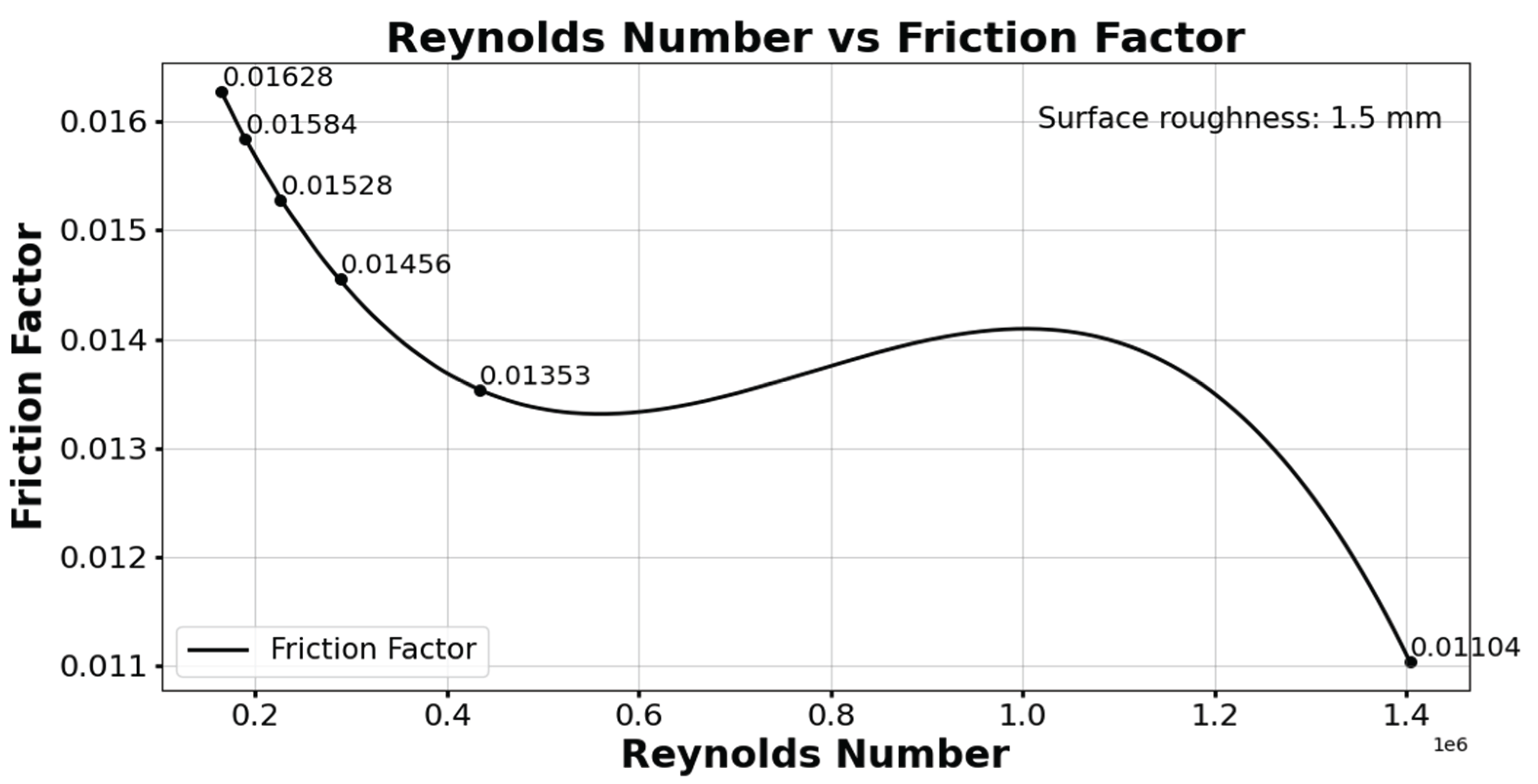
Figure 14.
Reynolds Number and friction factor relation for different surface roughness values.
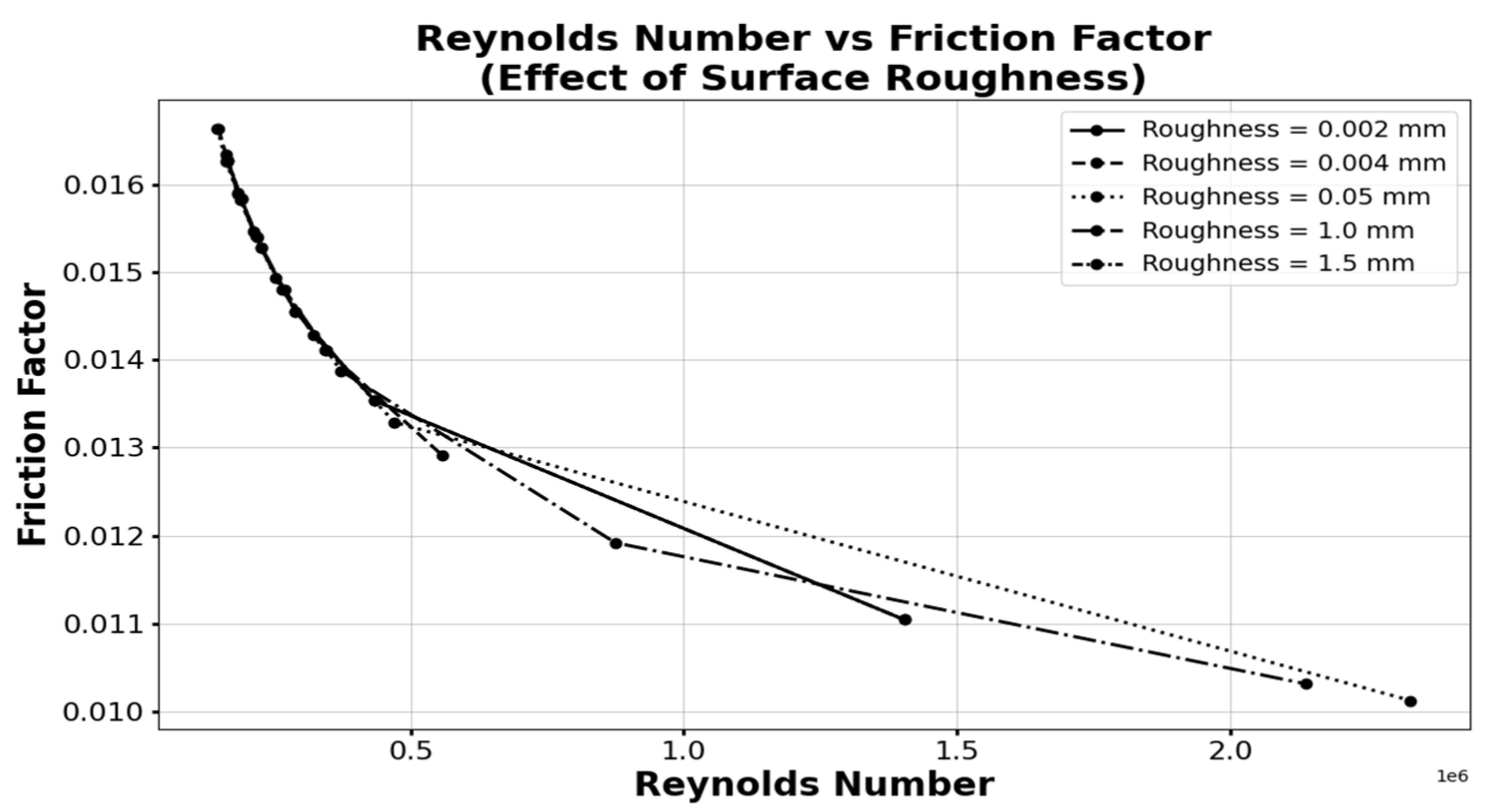
Figure 15.
H2 Pressure losses over a distance of 100m for different gas pressures (rough ness = 0.02mm).
Figure 15.
H2 Pressure losses over a distance of 100m for different gas pressures (rough ness = 0.02mm).
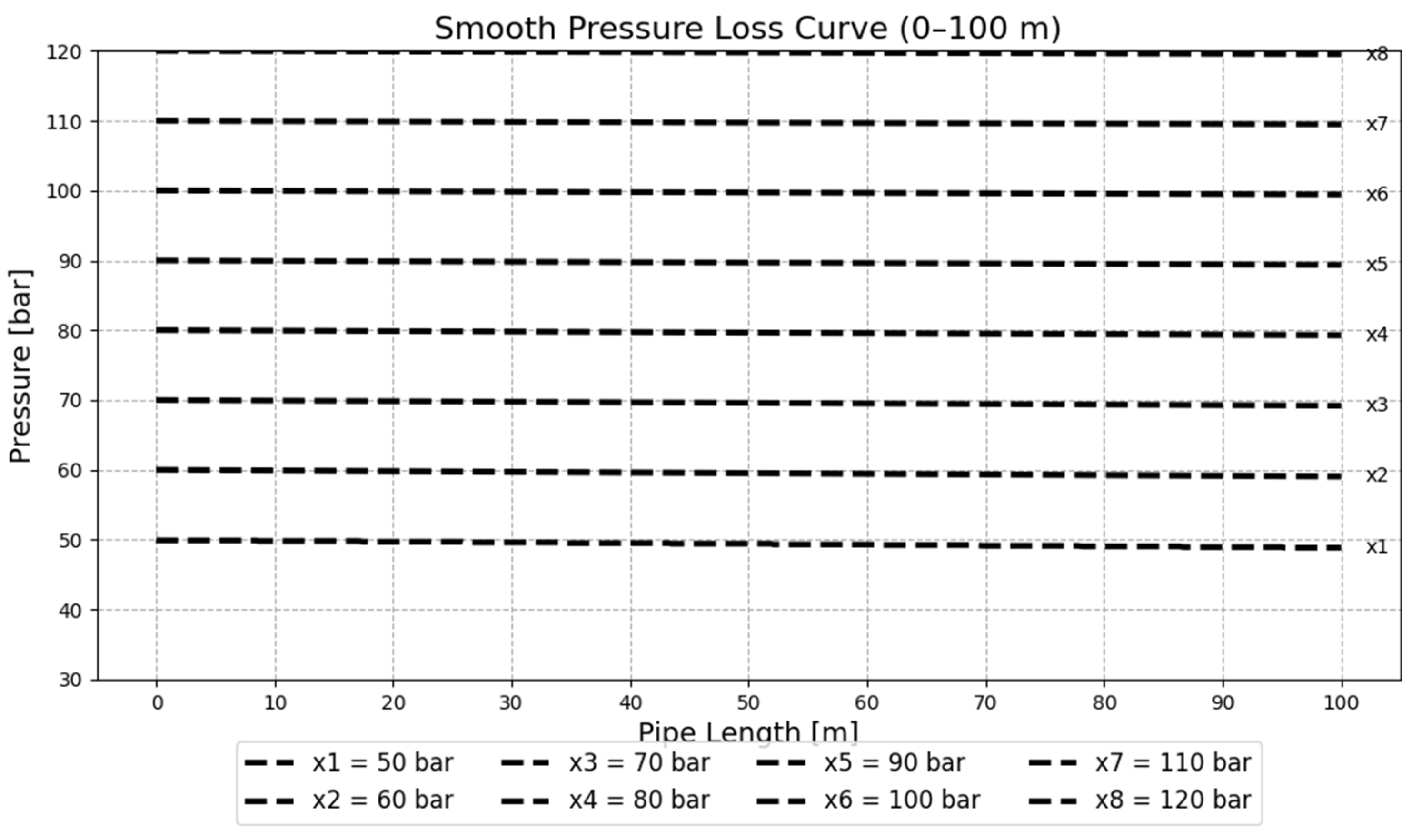
Figure 16.
Velocity profile of H2 gas in pipeline for surface roughness 0.02mm.
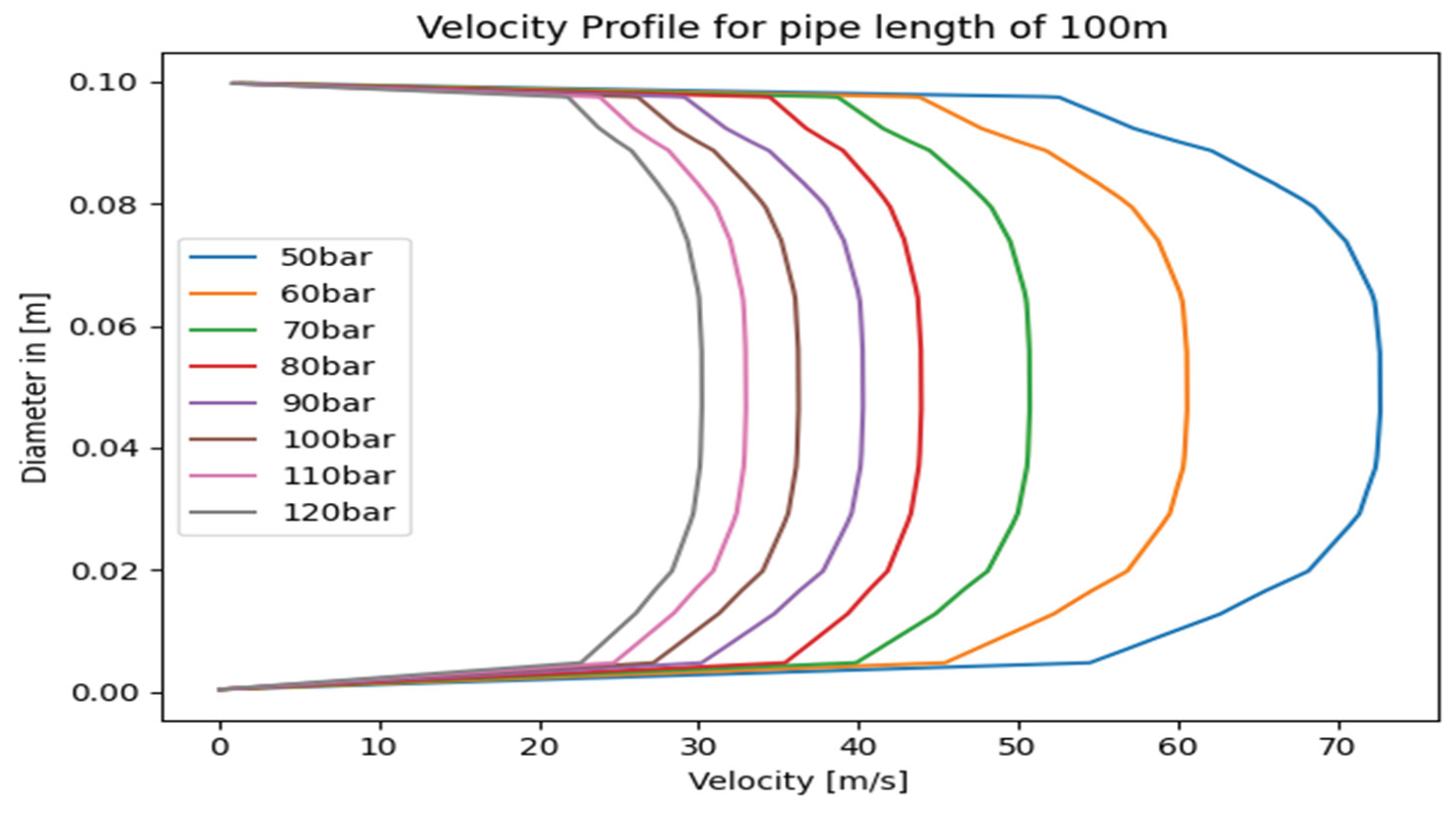
Table 1.
Pressure loss for 100km with material roughness 0.02mm using AGA.
| Initial pressure in bar | Final Pressure in bar | Pressure Difference in bar | Velocity m/s | Reynolds Number | Friction factor |
|---|---|---|---|---|---|
| 50.00 | 20.08 | 29.92 | 77.25 | 792606.00 | 0.014896 |
| 60.00 | 30.77 | 21.23 | 50.41 | 517220.00 | 0.015377 |
| 70.00 | 52.95 | 17.05 | 29.29 | 300523.00 | 0.016257 |
| 80.00 | 65.60 | 14.40 | 23.64 | 242552.00 | 0.016668 |
| 90.00 | 77.48 | 12.52 | 20.02 | 205410.00 | 0.017022 |
| 100.00 | 88.90 | 11.10 | 17.45 | 179041.00 | 0.017349 |
| 110.00 | 100.02 | 9.98 | 15.51 | 159136.00 | 0.017639 |
| 120.00 | 110.92 | 9.08 | 13.98 | 143438.00 | 0.017946 |
Table 2.
Pressure loss for 100km when the material roughness is 1.5mm using AGA.
| Initial pressure in bar | Final Pressure in bar | Pressure Difference in bar | Velocity m/s | Reynolds Number | Friction factor |
|---|---|---|---|---|---|
| 72.00 | 11.34 | 60.66 | 136.80 | 1403605.00 | 0.011043 |
| 80.00 | 36.67 | 43.33 | 42.30 | 434009.00 | 0.013534 |
| 90.00 | 55.17 | 34.83 | 28.11 | 288416.00 | 0.014555 |
| 100.00 | 70.31 | 29.69 | 22.06 | 226341.00 | 0.015277 |
| 110.00 | 83.93 | 26.07 | 18.48 | 189609.00 | 0.015836 |
| 120.00 | 96.66 | 23.34 | 16.04 | 164574.00 | 0.016275 |
Disclaimer/Publisher’s Note: The statements, opinions and data contained in all publications are solely those of the individual author(s) and contributor(s) and not of MDPI and/or the editor(s). MDPI and/or the editor(s) disclaim responsibility for any injury to people or property resulting from any ideas, methods, instructions or products referred to in the content. |
© 2026 by the authors. Licensee MDPI, Basel, Switzerland. This article is an open access article distributed under the terms and conditions of the Creative Commons Attribution (CC BY) license (http://creativecommons.org/licenses/by/4.0/).
Copyright: This open access article is published under a Creative Commons CC BY 4.0 license, which permit the free download, distribution, and reuse, provided that the author and preprint are cited in any reuse.


