Cost and Capacity Issues in Small Hospital Departments, Difficulties in Estimating Future Demand, the Impact of Seasonality, and the Cost Reduction (If Any) from Reducing Length of Stay

1. Introduction

1.1. Overview

This is part 4 in a series comparing international hospital bed numbers [1], bed demand and occupancy [2], and how to conduct ‘good’ hospital capacity planning [1,2,3]. This part is a linking study for both maternity [3] and pediatric capacity planning [4] due to their common reliance on trends in births as a primary factor in determining past and future bed capacity, and their relatively small size. They are used to illustrate issues common to many small hospital departments where the bed pool is reserved for a specific set of patients.

Given that pregnancy and birth are a fundamental part of healthcare planning it is surprising that in England over the last 35 years no guidance has been given regarding how to calculate the required number of maternity beds to support admissions for care during pregnancy and childbirth. How to make such calculations has seemingly been lost from the collective memory [3]. There is some guidance by the British Association of Perinatal Medicine regarding neonatal cot numbers and staffing [5], although the issue of determining cot numbers is somewhat vague. While a recent study outlined how to go about maternity capacity planning [3], a simple table linking annual births to the required number of available beds is lacking. Indeed, additional discussion regarding international trends in births is needed as is a more detailed examination of the issue of variable seasonality (timing and magnitude) in births with more explicit advice on the best way to calculate ‘seasonality’.

Regarding a potential births-to-beds calculator, the basis for such a calculator lies in the field of Poisson statistics and queuing theory. Poisson randomness was presented in the paper by AK Erlang in 1909 and subsequently developed to include implications to queuing theory with the Erlang B and other queuing equations [6]. It was first used to size telephone exchanges and is now used with great confidence in multiple industries to calculate how many servers (beds, midwives) are required to meet incoming demand at various levels of ‘loss’. i.e., the customers/patients must wait or go away [6].

Using queuing theory and the Erlang B equation to calculate hospital bed capacity was first suggested in 1954 [7] and for obstetric units in 1959 [8]. It is now widely used in academic literature for all aspects of maternity and pediatric capacity planning [3,9,10,11,12,13,14,15,16,17,18,19,20] where it is especially relevant to unscheduled care [12,15]. Erlang B should therefore be widely used in hospital capacity planning, but widespread ignorance seems to prevail among hospital managers and government agencies. Indeed, almost every study on the adverse effects of high hospital bed occupancy has ignored the effect of size on turn-away.

This study demonstrates how such tables can be generated and is validated using maternity unit data from England and the USA. In many ways, that is the ‘simple’ part, because Erlang B assumes a steady state whereas births involve considerable seasonality. In addition, forecasting future births entails considerable complexity and uncertainty and this will be presented using examples from around the world.

Issues regarding whether reducing length of stay (LOS) in short stay specialties such as maternity actually reduce costs are addressed in greater detail and it is proposed that most maternity costs, both direct and indirect, should be apportioned on admission rather than LOS. Using LOS creates the illusion that LOS is ‘expensive’ and must be reduced to save money. An irrational focus on reducing LOS then ensues which may not benefit the patient or reduce total system costs.

1.2. The Nine Fatal Errors in Capacity Planning

Over a 30-year career in hospital capacity planning I have noticed that poor advice is often given by external ‘experts’ leading to the construction of hospitals or departments which are too small to be fit-for-purpose. This has led to the formulation of nine ‘never make these fatal errors’ in capacity planning.

• Attempt to minimize capital and staff costs by devising the minimum case possible for all variables and assuming all schemes to reduce demand will simultaneously achieve 100% success. See point #8.
• Use simplistic age-based forecasts for admissions based on a single year of data. Instead use more than 8 years of data (preferably 15 years), to follow the trend in each year of age. Then take the trend into the future with multiple probable scenarios along with the observed (past) uncertainty associated with demand.
• Calculate avLOS based on midnight stays, always use real time data. Midnight LOS will consistently underestimate the real avLOS [3].
• Assume that avLOS is a constant, rather than a variable with confidence intervals, and assume that avLOS decreases ad-infinitum. Most trends in LOS decrease toward an asymptote because there is a biological limit to recovery and/or the effect of medications.
• Focus exclusively on those HRG/DRGs which show above average LOS. These will generally be matched by other HRG/DRGs with lower-than average LOS. These arise due to the ambiguities in the local clinical coding process compared to that applying to the national average. This includes how doctors record diagnoses and the depth of local coding with complications and existing conditions affecting health. Local LOS is subject to sampling error as it is a small subset of national data [21].
• Use annual averages for admissions and avLOS. Many conditions show seasonality due to multiple causes and LOS can also show seasonal variation.
• Assume that lower avLOS means better care or that lower avLOS makes large savings in costs. It is the volatility in admissions which dominates bed demand not the calculated avLOS – this directly contradicts the accepted dogma that reduction in LOS is one of the key ingredients to reducing bed demand. Reducing LOS only benefits a steady state system (such as elective/scheduled care) or the baseline bed demand which lies beneath the volatile changes in emergency/unscheduled care, see I.6,9 in Supplementary material S1 of [3]
• Assume that 85% occupancy is a proven figure. Proof of 85% as an optimum occupancy does not exist and most categorically does not apply to small bed pools, see references and discussion in [1,2,3].
• Make simplistic models comprising all the variables and proposed schemes to reduce admissions and LOS. An alternative is to use Monte Carlo simulation (including seasonality) which will show the full range of probable outcomes. This is a subset of operational research [22,23,24]. The alternative is to use past data to illustrate the sources of variability – upon which Monte Carlo simulation will be based but without the full nuances of the real world. Hence simultaneous variation in admissions and LOS imply that the actual trend in occupied bed days is a preferred approach.

The nine fatal errors have been regularly observed by the author relating to capacity planning in England [1,2,3]. These were forced on the English NHS in an environment where politicians had an erroneous belief that the NHS had too many beds in addition to a serious policy fiasco where the Private Finance Initiative (PFI) for building hospital capacity necessitated government Treasury rules for the affordability of PFI projects, where the fiscal rules contradicted the real world of how bed demand behaved [1,2,3].

These nine fatal errors apply across all aspects of hospital bed planning and are illustrated in both the maternity [3] and pediatric [4] capacity planning studies.

2. Materials and Methods

2.1. Sources of Data

Data relating to births and available beds for US maternity units in 2000, 2009 and 2019 was from the study of DeSisto et al. [25] while data for English maternity units was from NHS maternity statistics for births in 2023/24 [26], and for available beds in 2023/24 from the NHS England bed availability KH03 series [27]. Neonatal unit data is from, winter daily SITREPS [28].

International births were from the United Nations [29], annual births in the USA [30], births in Arizona [31] and Hawaii [32]. Monthly births in European countries from Eurostat [33], and annual births in Australian regions [34].

Monthly deaths by age and sex, England and Wales [35]. Data relating to vaginal delivery and cesarean section (C-section) in Australian hospitals [36].

2.2. Additional Data from English Hospitals

Additional data covering births in 2023/24 split by site were obtained by Freedom of Information requests to larger English NHS Trusts.

2.3. Estimating Births in Auasralian Hospitals

Data regarding the number of admissions at each Australian hospital for vaginal delivery and cesarean section [36] were added together and this total was then uplifted to total births in 2023 [34]. Hospitals were then grouped in 1000 increments in births up to >7000.

2.4. Births in US Hospitals by 1000 Birth Increments

Data from DeSisto et al. [25] covers only 7 broad intervals up to 7000+. The first 3 bands up to 999 births were added together. Above 1000 each broad band was approximately split, i.e., band 4000 to 6999 was split into 5 bands to give a smooth transition between the adjacent bands, namely,2000 to 3999 and 7000+. For the purpose of plotting data onto a chart high precision is not required

2.5. Births in US Hospitals and the Ratio of Births per Bed

Data from DeSisto et al. [25] covers 7 broad intervals up to 7000+. For the purpose of plotting births versus available beds per 1000 births data on a chart, births were taken as a single value by estimating that the average was reasonably close to the maximum value in each band. High precision is not required.

2.5. Linking Births and Beds for English Hospitals

For each NHS Trust annual births and beds were linked in an Excel spreadsheet. For the larger NHS trusts a Freedom of Information request was sent to obtain the number of births at each site run by the Trust.

2.6. The Line for 0.1% Turn-Away

Data from the Erlang equation at 0.1% turn-away was taken from Jones [3,4] where occupied bed days were converted to births by assuming that each birth was associated with 3.2 occupied bed days per birth. This is the total of all bed days (in real time) associated with admissions during pregnancy and during childbirth, but excluding time spent in the birthing unit. The tabular data of Jones [3,4] goes in 1 bed increments up to around 50 beds and wider increments (usually 5 beds) were converted to 1 bed increments by linear interpolation.

3. Results

3.1. Defining a Bed Pool

A bed pool is a collection of beds dedicated to a set purpose such as adult/child, maternity/other care, the critical care unit, the birthing unit, etc. Other types of care are not allowed to cross into the defined bed pool and most importantly the bed pool size must be determined at each site if the organization operates across multiple sites.

The bed pool then becomes the fundamental unit for capacity planning. The planner must therefore understand which patients use the different bed pools. In most instances this can be achieved using the ward name. Some discretion is also allowed if patients can be quickly transferred between sites to balance demand among the smaller bed pools. These become intra-organization transfers as opposed to officially recognized inter-organization transfers.

Smaller hospitals will increasingly rely on transfers to larger hospitals for the care of more complex patients, and adverse outcomes may then show up in the hospital receiving such patients.

In the case of small community/rural hospitals, out of necessity, the hospital itself may well become the multi-specialty bed pool.

3.2. Maternity and Pediatric Units at the Same Location Have a Smiliar Size

This study forms a common overlap between maternity and pediatric capacity planning and so it is useful to note that when located at the same hospital they both have a similar size.

In this analysis, occupied rather than available (staffed) beds are used to avoid additional uncertainty arising from both units operating at different levels of turn-away. The data is from NHS England quarterly bed statistics and covers the years 2022/23, 2023/24 and 2024/25 [27]. The data covers hospitals which have both a maternity and pediatric unit, i.e., it excludes Children’s hospitals without a maternity unit such as Great Ormond Street and vice versa, and excludes any LOS associated with same day stay admissions.

The data is structured as follows. On the left-hand side is quarterly data for individual hospitals, next comes annual data at the same hospitals and then quarterly and annual data covering English regions and finally on the right is the ratio for the whole of England.

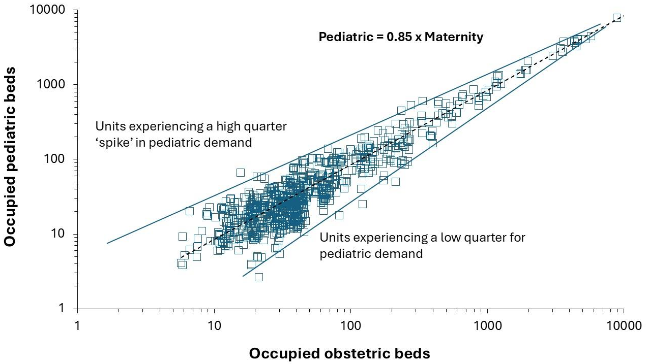
Figure 1 displays the data for all English hospitals which have both a pediatric and a maternity unit, then data for English regions where the ratio will also include free standing women’s and pediatric hospitals and finally data for the whole of England.

Figure 1 shows that there is greater scatter in the quarterly data simply because pediatrics show a different pattern and higher seasonal behavior [3,4]. In England, seasonality is mainly restricted to higher births around September [3]. In addition, the scatter increases as the size of the unit decreases, which is an expected outcome from Poisson-based randomness in arrivals and case-mix variation from different populations.

However, when looking at specialty totals across England (excluding mental health) over the years 1998/99 to 2023/24, where bed days includes a contribution from same day admissions, it is observed that occupied beds for specialty pediatrics (specialty code 420) versus maternity (obstetrics plus midwifery) account for 5.6% to 6.8% of total acute occupied beds while maternity only accounts for 3.5% to 4.5% of the total. This data source will attribute LOS in Children’s hospitals to the pediatrics total.

The ratio between pediatrics and maternity will vary between countries especially if the average LOS is markedly different to that in England, and if real time LOS is used [3]. The scatter at regional level will also dflowse because of the unequal distribution between free standing children’s and women’s hospitals which will distort flows to nearby surrounding general pediatric and maternity units.

In conclusion, whatever the exact ratio, both specialties are small in relation to total acute care. Due to the relationship between size and bed occupancy (see later) it is important to use real-time occupied bed days rather than available beds although both metrics could be presented. The main point is that similar sizes imply approximately the same issues with economy of scale. In addition, a small pediatric/maternity unit will usually imply a small hospital.

3.3. How Many Beds Are Needed for Various Levels of Births or Admissions?

As presented in previous studies [2,3] the Erlang B equation can be used to link available beds, bed occupancy and turn-away. Turn-away measures the proportion of time that a bed is not immediately available for the next patient and is therefore a measure of delays to treatment, hidden queues, cancelled operations, transfers to other hospitals and operational chaos.

All Erlang calculators exist to help make management decisions by performing alternate calculations under various assumptions. The output must always be compared against real data. Never use annual averages as the idea is to estimate peak demand.

To assist hospital managers two bed calculators will now be discussed and are available in Supplementary material S1., namely:

• A modified Erlang B calculator using births and bed days per birth, which calculates required beds at an assumed 0.1% turn-away.
• An Erlang B calculator using daily admissions and average length of stay which shows average occupancy and turn-away for 1 bed increments in available beds.

Given that all care during pregnancy and childbirth requires immediate attention a turn-away of 0.1% or less is recommended. Strictly speaking the admission rate and length of stay associated with the peak month for births should be used since an annual average will underestimate real bed requirements. This is covered in the section regarding seasonality. If the unit is currently operating at high turn-away, then the total bed days per birth will be lower than the required level and will need an uplift. One solution is to estimate the bed days per birth during the months when births are lowest and turn-away will also be lower.

Erlang depends on accurate length of stay (LOS) which must be derived from real time data. Average LOS based on midnight stays give averages which are lower than reality [3]. In addition, an allowance must be made for the time it takes to get the bed ready for the next patient. There is no point in fooling yourself by feeding a low LOS figure into the model.

3.3.1. A Births-to-Beds Calculator

The first calculator is a births-to-beds calculator which uses outcomes from Erlang B which meet the criteria of 0.1% turn-away, however, it uses the expected number of annual births (a readily available statistic) and the ratio of total bed days per birth. This is found in the Read Me 1 section of the spreadsheet in Supplementary material S1. A calculator at 3% turn-away is also given, and the base data is provided in another tab. The reason for the 3% turn-away calculator is given in the discussion.

For the maternity unit total bed days include all stays during pregnancy and after discharge from the birthing unit. For the birthing unit this will simply be the average stay in the birthing unit. For the neonatal unit the total bed days will be directly from that unit divided by the total births. Hence there is a hidden conversion for the proportion of births that are admitted to neonatal critical care. The same reasoning applies to any ambulatory ‘assessment’ units whose beds and occupancy must be calculated separately.

This calculator asks the user to input the value for seasonality in cell A2. This is a locally derived figure or nearest estimate from a later section dealing with seasonality.

This calculator also shows the ratio of required beds per 1000 births which is a measure of bed throughput. It immediately reveals that smaller units rapidly lose economy of scale and incur inescapable and escalating costs per birth.

Table 1 illustrates the output from this calculator at three different levels of total bed days per birth. In this example no adjustment has been made for seasonality. For each increment in available beds the annual births column shows the maximum births consistent with 0.1% turn-away. The next column shows this as a ratio of beds per 1000 births. The ratio of beds per 1000 births demonstrates that diseconomy of scale is operating powerfully below 10 beds.

As can be seen in Table 1, a 6-bed unit can only accommodate 131, 105 or 84 births at 3.2, 4 or 5 total bed days per birth. Such small units are usually not resourced for complex patients and/or will not have neonatal capacity and so mother/baby will be rapidly transferred to a larger unit. Hence their effective bed days per birth will be lower than the 3.2 bed days per birth in the first column.

The calculator also contains provision to input variables relevant to the birthing unit such as day-of-week (cell A3) and hour-of-day (cell A4). The study of Dexter and Macario [14] describes the day-of-week and hour-of-day factors relevant to birthing units.

Should you wish to check the overall size of an Obstetric or midwife-led unit using this calculator then use the same number of annual births but the total bed days per birth will be the sum of all LOS (in real time) across all types of beds such as antenatal/postnatal, birth centre, labor ward, triage or recovery beds. This will give a total unit size which is slightly too small due to the economy of scale implied by the larger total of beds. As a rough guide, total beds should be around 1.3- to 1.4-times the number of maternity beds. The higher figure is likely for an Obstetric unit while the lower figure for a mixed Obstetric/midwifery unit.

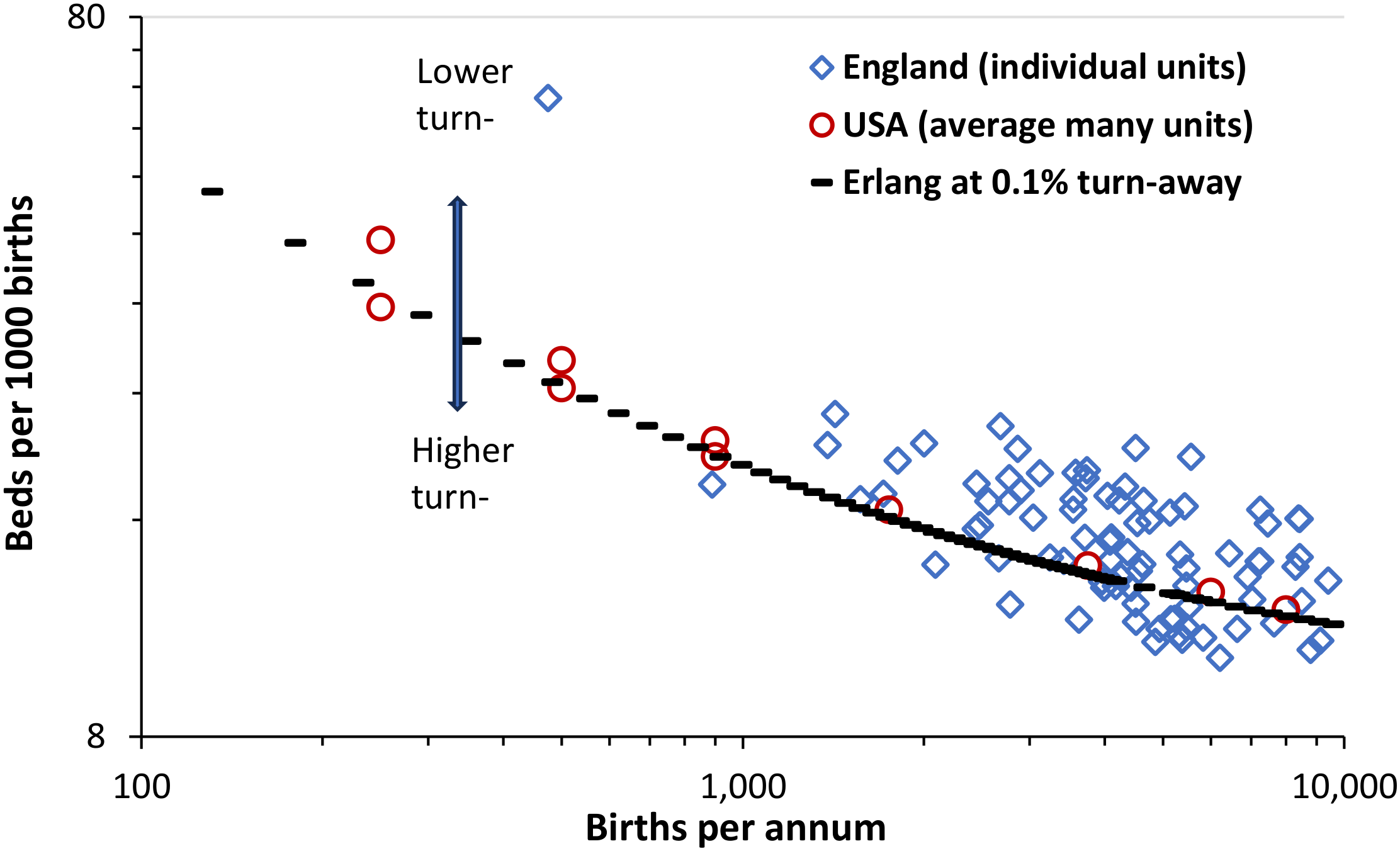
The output from the births-to-beds calculator has been checked against the real world where Figure 1 shows the relationship between available beds per 1000 births and births for each of two data sets., namely individual maternity units in England [26,27] and national averages for units of different sizes in the USA [25]. Data for the USA is the highest and lowest values observed over the years 2000 to 2019. Data for England has been trimmed to exclude implausibly high/low values. Regarding implausibly low figures for bed occupancy I have contacted a number of Trusts and have discovered that a significant number are incorrectly reporting total birthing plus maternity beds as the ‘maternity’ bed count while matching this against the occupied beds in the maternity unit.

Figure 2 uses the ratio of beds per 1000 births to illustrate the effect of size on bed utilization as shown in Table 1. As can be seen both the US and English data lie along the line described by the Erlang equation at 0.1% turn-away. England will have slightly higher LOS than the USA hence the data lies slightly above that for the USA.

There is some scatter in the English data simply because around half of English units operate above 0.1% turn-away [3].

For context, the smallest general maternity unit in England has around 10 beds because England has far higher population density than the USA. England and the USA tend to operate at very low length of stay compared to other countries [34]. By way of comparison there are around 23.3 to 25.9 beds per 1000 births in Belgium where 37% of maternity units are in the range 500-1000 births per annum and the three largest units have just over 3000 births p.a. [39,40].

The issue of forecasting future births is covered later, with a birth forecasting tool presented in Supplementary material S2.

3.3.2. A Calculator Using the Erlang B Equation

The second calculator uses the Erlang B equation [12] where the daily admission rate and average length of stay are entered. In Supplementary material S1 this calculator is found in the Read Me 2 section.

To those unfamiliar with Erlang B the equation has two parts, namely, a top part which is divided by the bottom part. Erlang B involves the manipulation of very large numbers which even computers struggle to handle, however, the calculator will handle almost all scenarios applicable to maternity units especially below 30 beds. Above 30 beds multiple Erlang B calculators can be located by an internet search. These use a variety of estimation methods to handle the very large divisions required by Erlang B.

The sheet ‘Turn-away and occupancy’ is where the daily admission rate and average length of stay (avLOS) are input and the user simply scrolls along row 4 to find the number of beds compatible with the desired level of turn-away. Row 6 gives the average occupancy at this level of turn-away while row 8 shows the average number of occupied beds. This calculator can be used for all types of bed pools including the maternity ward, the birthing unit, neonatal critical care, pediatric units, a cardiac ward, etc.

The excellent study of Dexter & Macario [14] gives an example of how to use this calculator when there are day of week and hour of day patterns in the arrival rate and bed occupancy. Also note that day-of-week factors will be required to cope with the impact of ‘elective’ maternity (such as C-sections, etc.) admissions. In parturition there is some discretion to move otherwise unscheduled events to scheduled intervention. Hence the arrival rate will have to be adjusted upward to account for the general Monday to Friday workload from any ‘elective’ events.

In the case of small community/rural hospitals where pregnancy and childbirth are part of a wider mix of services then it is appropriate to use the admission rate to the entire hospital (all specialties) and the resulting whole hospital avLOS become the inputs. Use historic data to scan for seasonal profiles and if bed demand varies by day of the week and hour of day. Adjust the inputs into the calculator appropriately.

Finally, never assume that avLOS is a constant and check for any seasonal variation as the case mix subtly changes.

3.3.3. Comparing Different Sized Units

Previous studies have used Erlang B loss tables to show multiple lines of constant turn-away where the unit size and average occupancy is input, thereby allowing a like-for-like comparison between multiple units of disparate sizes [2,3,4].

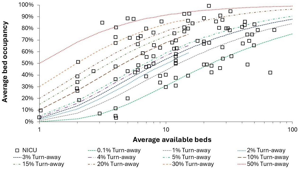
Figure 3 shows the situation for neonatal intensive care units (NICU) in England for the autumn/winter/spring period in 2024/25. Occupancy and turn-away for these units in the winter of 2023/24 has been previously reported [3]. A surprising number of units operate above 20% turn-away, which has never been investigated in terms of adverse outcomes. This type of chart is recommended for regulatory agencies.

NICU is characterized by high levels of immediate access but with only around 20 units correctly functioning near to or below the 0.1% turn-away line. English units tend to operate in a hub and spoke arrangement centered around larger regional hospitals (lying at the right-hand side of Figure 2), however, units above the 20% turn-away line almost certainly need more beds. For both PICU and NICU in England [2,4] several units operate above 85% average occupancy and will therefore experience the combined deleterious effect of high turn-away and high busyness. Compared to the USA England has fewer NICU per 1000 births and this is reflected in higher overall turn-away in Figure 2.

Regarding the level of safety for maternity units, note in Figure 2 that around 20 units consistently function above 85% average occupancy. Based on the principle of the link between busyness and patient safety [2,3], such units should be on the hospital’s risk register and questions should be raised as to why this situation has not been addressed. Recall, that turn-away is a risk factor but that the expression of this risk depends on the level of staffing (which is sometimes approximated by the 85% occupancy figure).

3.3. The Size of Maternity Units in Different Countries

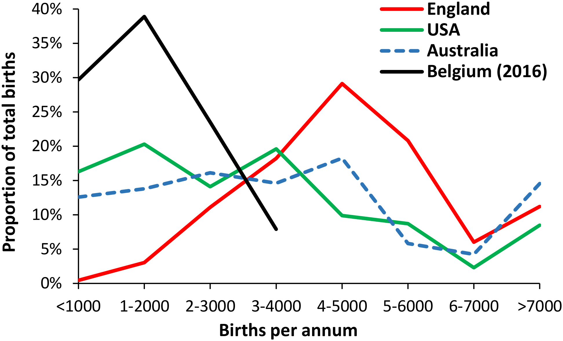
While the USA has several large cities only two states have more than 1000 persons per square mile (equal to 390 persons per square kilometre) [41]. Over 90% of the surface area is low density rural areas [41]. This implies a disposition to small maternity units commencing with just 1 (nominal) bed [25]. In contrast England has very high population density and this reflects in almost all maternity units above 10 beds (1000 births). Australia has another geographical distribution with large cities along the coastline. Prior to 2019 Belgium had a system focussed on numerous small units [39,40]. These are illustrated in Figure 4 where the distribution of maternity units by size in Australia is somewhat similar to the USA due to a disparate rural population. Belgium had a very high proportion in the two bands >2000 births per annum – although this will undergo rationalization once the legislation is passed [39,40].

The data for England has been broken down to the level of single sites while that for the USA may include some organisations operating from multiple sites, especially in the >7000 births category. This disparity in size has huge implications to capital costs and the cost per birth in each country, i.e., due to low population density the USA is structurally expensive due to capital costs per birth and with additional disparities in salaries between the USA and England. The assumption is that Belgium is structurally more expensive than the USA, although the USA has a far longer tail in the <1000 birth category.

3.4. International Trends in Births

Given that both maternity and pediatric services are related by the trends in past and future births, such trends are an important aspect of capacity planning. [3,4]

The previous study investigating maternity bed capacity [3], it was suggested that births in England could rise by up to 24% higher than in 2023 over the next 15 years. An expanded birth forecasting tool is available in Supplementary materials S2 which is also relevant to pediatric capacity planning [4]. The dilemmas surrounding forecasting future births are addressed later.

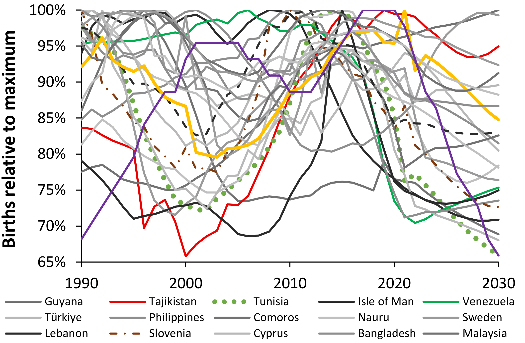
To illustrate the diversity of the trend in births overtime Figure 5 shows the birth profile of 25 world countries between 1990 and 2023 with a forecast through to 2030 [29].

As a point of comparison, the ratio of the maximum to minimum births for 239 countries ranges from just 1.03 in Bolivia to 5.8 in Montserrat, with a median value of 1.7. Values for the USA and UK are 1.16 and 1.21 respectively. The ratio for the world population is 1.11 due to high growth countries (mainly Africa, Afghanistan, Iraq, etc.) counterbalancing those with declining births (mainly India, Nepal, Asia, South America, etc.).

Each country reflects a unique combination arising from the timing of previous births, government birth control policies, net migration, economic cycles, etc.

Note the somewhat artificially smooth trends produced by the World Bank for the period 2024 to 2030. This issue was covered previously [3]. The key message from Figure 5 is to never assume straight line trends.

3.5. The Dilemmas Regarding Forecasting Future Births

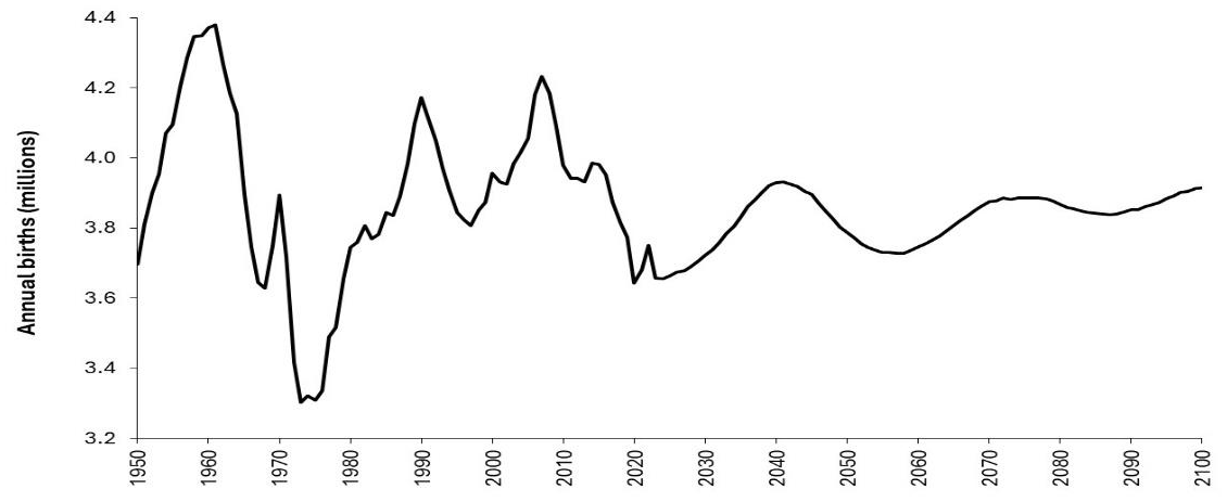
While it is true that the fertility rate is decreasing around the world [42], it is not true that the number of births is decreasing in every country (as in Figure 5) or location. The previous study on maternity capacity planning [3] devoted considerable attention to the unreliability of birth forecasts and the local factors affecting these trends. To illustrate these concepts Figure 6 shows the trend in births for the USA between 1950 and 2024 along with a forecast to 2100 [30].

The trend for the USA encompasses the combined effects of past trends in births, immigration, birth control, and fertility rates, and how these have a knock-on effect in the present and future. It was previously noted that England has a similar cyclic pattern to the USA arising from the World War II baby boom [3] while Figure 5 suggested that cyclic trends are fairly common in disparate countries, although probably with different causes.

Each maternity and pediatric unit sits within a bigger national, regional and local context which must be understood to construct reasonable scenarios for future demand. National and state statistical agencies will have the relevant data and may be able to assist with local birth forecasts under various assumptions. Key factors will be approval for new dwellings and potential expansion/contraction of major local employers.

3.6. Local Trends in Births

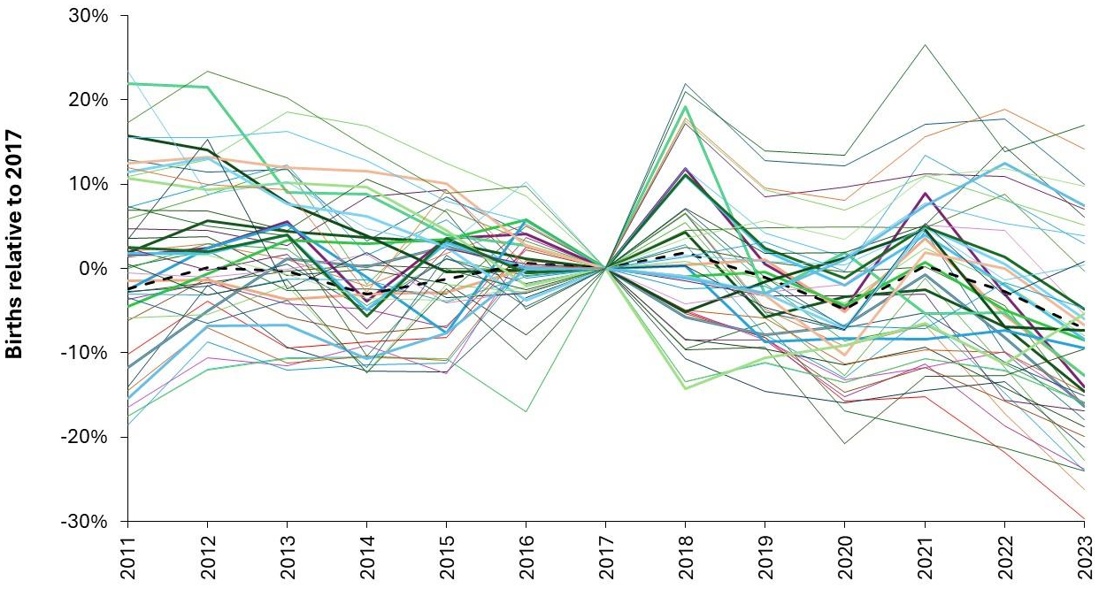
To further illustrate the issue regarding local trends, Figure 7 shows the trend in births from 2011 to 2023 relative to 2017 in selected Australian regions.

Australia has around 300,000 births per annum (black dashed line). Most regions have over 1,000 births per annum but the smallest region, namely South East Tasmania, has less than 400 per annum. Figure 7 demonstrates the highly regional nature of birth trends and that even at regional level there is considerable volatility between years.

Even at the level of Australia (black dashed line) there are occasional minimum years as in 2014, 2020, 2023.

The minimum in 2020 (-3.7% compared to 2019) is repeated in other countries, despite an almost total lockdown in Australia including international travel, i.e., COVID-19 infection per se is an unlikely cause. In England and Wales, the minimum births in 2020 only commences from June 2020, i.e., conceptions after November 2019, which is before the arrival of COVID-19. Births stay depressed until the 12-months ending June 2021 and then show a significant surge for the 12-months ending February 2022, i.e., conceptions before June 2021. Hence, while tempting to invoke COVID-19 the real cause(s) may lie elsewhere.

However, even for Australian regions with 1000 births the change ranges from -12% to +6% (1 STDEV of Poisson variation is ± 3%). Changes for the other years will have various contributory factors.

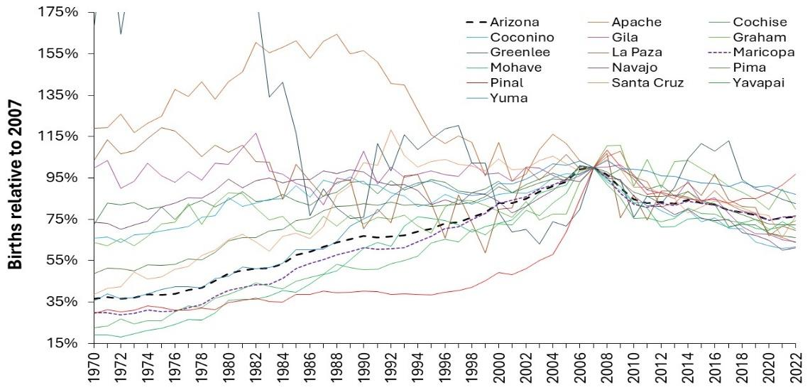
Finally, returning to the USA, Figure 8 [31] shows the trend in births for counties in Arizona.

These trends are unlike that for the USA in Figure 6 and look to be dominated by population changes especially in Pinal (5127 births in 2022, 31 persons per km²) and Greenlee (114 births, 2 per km²) counties. Hawaii also shows a maximum in 2008 followed by a 22% decline to 2023 and no immediate sign of reaching a minimum [28]. The importance of local factors cannot be overstated. A forecasting tool to estimate future births is provided in Supplementary material S2, however, it relies on local knowledge.

3.5. Using Births to Forecast Pediatric and Neonatal Admissions

Given that both maternity and pediatric services are related by births, Figure 1 [27] explored the relationship between the respective size of these units in the same hospital or region. In England, a pediatric unit has around 85% of the number of occupied beds as an associated maternity unit, with wider variation in this ratio as the hospital gets smaller or the comparison is made based on quarterly data.

The previous study investigating maternity bed capacity [3], it was suggested that births in England could rise by up to 24% higher than in 2023 over the next 15 years. A birth forecasting tool is provided in Supplementary material S2. Data in S2 is specific to the UK but can be adapted to other countries when used in combination with local knowledge.

The approach taken in S2 is to gather data on births at a local government level over a 20-to-30-year period or more. Since the UK has a strong cyclical pattern, this is used to estimate the next cycle. This approach can also be used for other countries such as those in Figure 5. In the absence of cyclical trends, a number of potential trends can be explored. Any available government statistical agency forecasts should also be considered to arrive at a number of alternate scenarios. A moving 12-month total of local births can then be used to see which scenario looks to be the most viable.

Supplementary material S3 presents one potential tool for forecasting pediatric (or other) demand. The main point of the forecasting tool is to force the use of single year of age in the understanding of why pediatric demand is so volatile. The issue of single year of age behavior in pediatric deaths will be explored in the discussion.

The sheet ‘Forecast admissions’ in S3 is used to circumvent the key problem that the catchment area of a hospital is not exactly known. However, births, neonatal and pediatric admissions and bed days are known for the unit wishing to forecast future capacity – assuming that the pediatric and maternity units are reasonably close by. Alternatively use births for nearby geographies for which data is available.

In ‘Forecast admissions’ data has been added for births to the residents of Milton Keynes in England where actual data is available up to 2023. Neonatal and pediatric admissions are merely example data from national ratios. Neonatal admissions assume an approximate ratio of 1 neonatal admission per 7 births (see below). Each unit will substitute their own actual births and admissions data.

Note how the forecast admissions rely on a cascade of ages arising from births. Hence births in 2002 become the population of 1 year-old in 2003, while births in 2011 become the population of 14-year-old in 2025, etc. For the sake of simplicity childhood deaths and inward/outward migration are ignored. The unit will also substitute their best forecast for future births (as alternate scenarios).

The aim of the sheet in S3 is to calculate a time series for admissions per birth/population by single year of age over 10 to 15 years to visualize the extent to which the trends in admissions show variation over time. The next step is to attempt to estimate how the admission rate will trend over time. In the example shown in the ‘Forecast admissions’ sheet the maximum admission rate from the past has been chosen to estimate the likely worst-case years in the future. The worst case will not simultaneously happen for all ages. The sheet shows that the variable admissions are dominated by the first year of life.

This approach has a major limitation in that its usefulness decreases as the size of the unit decreases and it will therefore give results dominated by Poisson randomness in small units which will include most US pediatric units. In such cases it can be used at State or Area Health Board level to gain insight into the fundamental issues surrounding uncertainty in capacity planning.

A highly recommended alternative is to substitute occupied the larger number of bed days instead of admissions. Since beds numbers are the goal the occupied bed days (average occupied beds = bed days ÷ 365 days per annum) approach is highly recommended. This sheet gives an annual average and an adjustment for seasonality will be required which can be achieved by an analysis of past daily occupied beds which is covered in the pediatric study [4].

As mentioned in the birth trends section the difficulty comes when attempting to forecast the future.

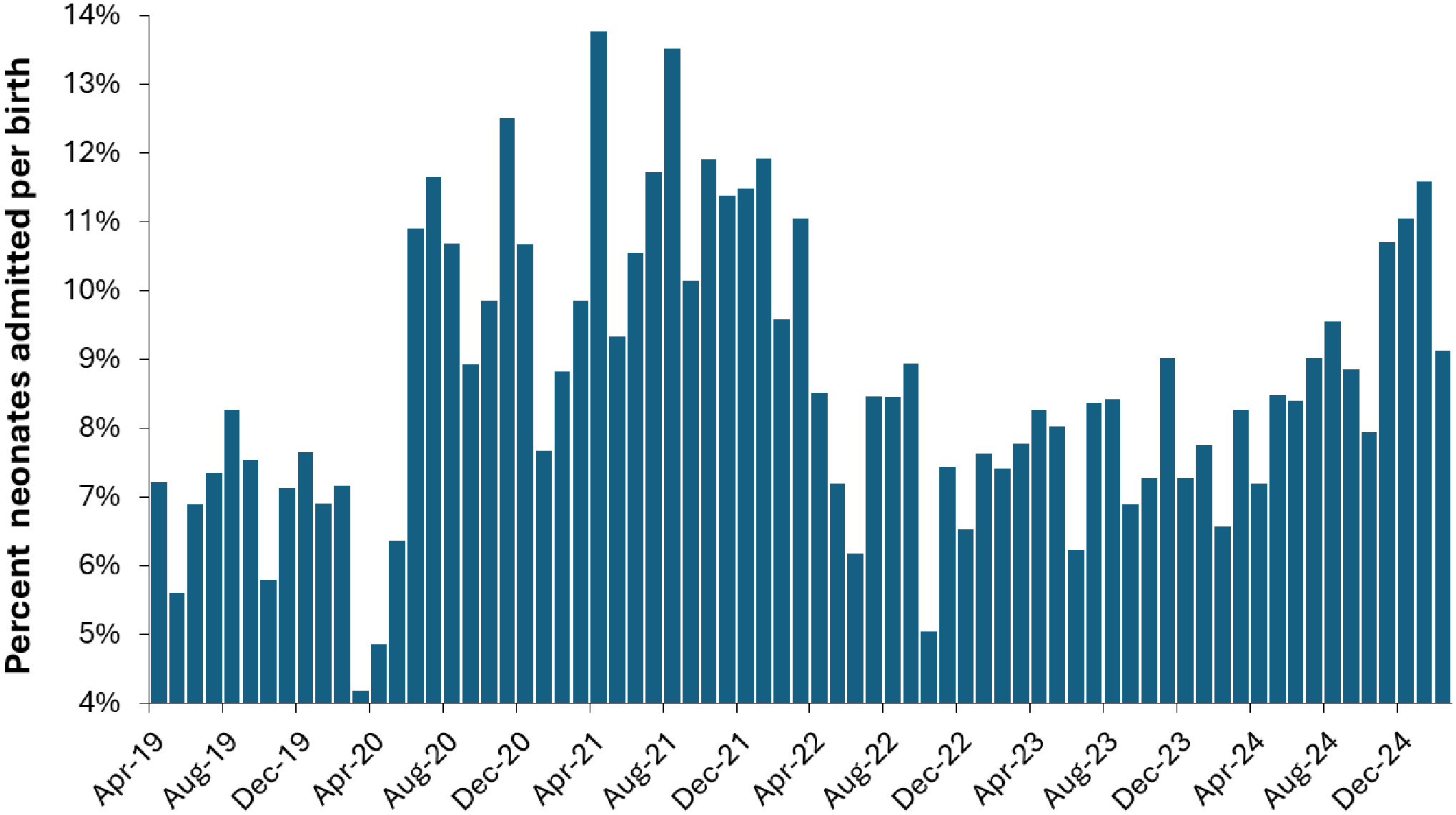
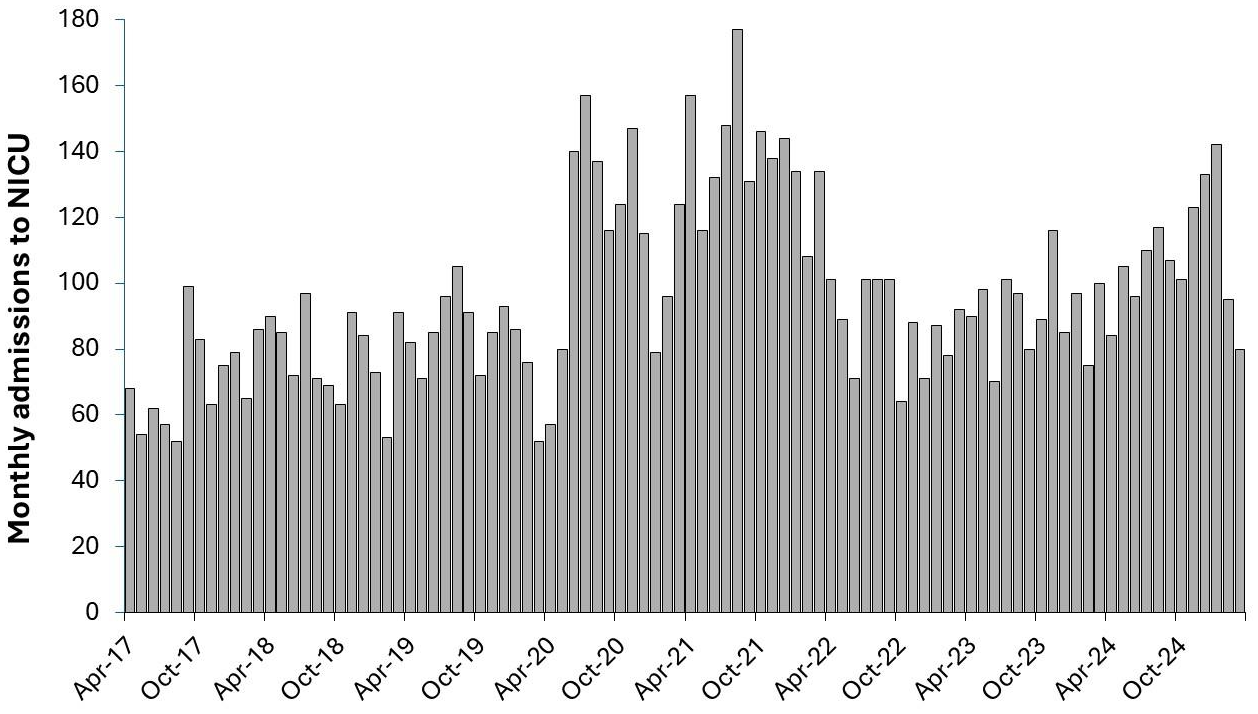
3.7. Issues Specific to Neonatal Intensive Care

Regarding neonates, Figure 9 shows that the proportion of births resulting in an admission to the neonatal unit shows systematic variation. Note that the actual monthly admissions shown in Figure 10 are the combination of births x proportion progressing to NICU. The data in Figure 9 and Figure 10 comes from a Freedom of Information request to the St Bartholomew’s (Barts) group of hospitals in London.

While it is tempting to assume that the first peak in Figure 9 is due to COVID-19, it is important to point out that the timing does not exactly coincide, and the data does not reflect the minimum points in the summer for COVID-19 infections. It is not widely appreciated that COVID-19 had a profound effect on the frequencies of pathogens via pathogen interference [4], and that lockdowns only temporarily altered the transmission of different pathogens. In addition, many neonatal conditions originate during pregnancy, especially during the first trimester. Hence births from April-20 onward will be influenced by events during the preceding 9 months of pregnancy.

Figure 9 and Figure 10 also demonstrate that annual averages can be very misleading. Indeed, due to the systematic changes in the ratio of neonatal admissions per birth, a 12-month total will give different answers depending on when the 12-month starts and finishes. This is called the calendar year fallacy.

Hence the actual admissions to NICU are a complex combination of the (variable) seasonality in births and the (variable) proportion of births progressing to the NICU. It would seem that irrespective of the trend in births that NICU admissions are increasing over time and show periods of high demand. The period of high demand during the first two years of COVID-19 should be investigated to see if the spectrum of diagnoses associated with admission was different to ‘normal’ [43]. However, note that admissions during the winter of 2024/25 were nearly as high as the two peaks during the first 2 years of COVID-19.

Note that the age in weeks for admission of premature neonates is decreasing over time as technology and medications improve [44], and that a higher proportion of births result in a NICU admission where the mother is aged over 30 years [44,45]. Also note that very preterm babies have a higher PICU admission rate in the first 2 years of life [44,45]. This brings us back to the issue of uncertainty about future demand and the need for flexible floor space to cope with future uncertainties.

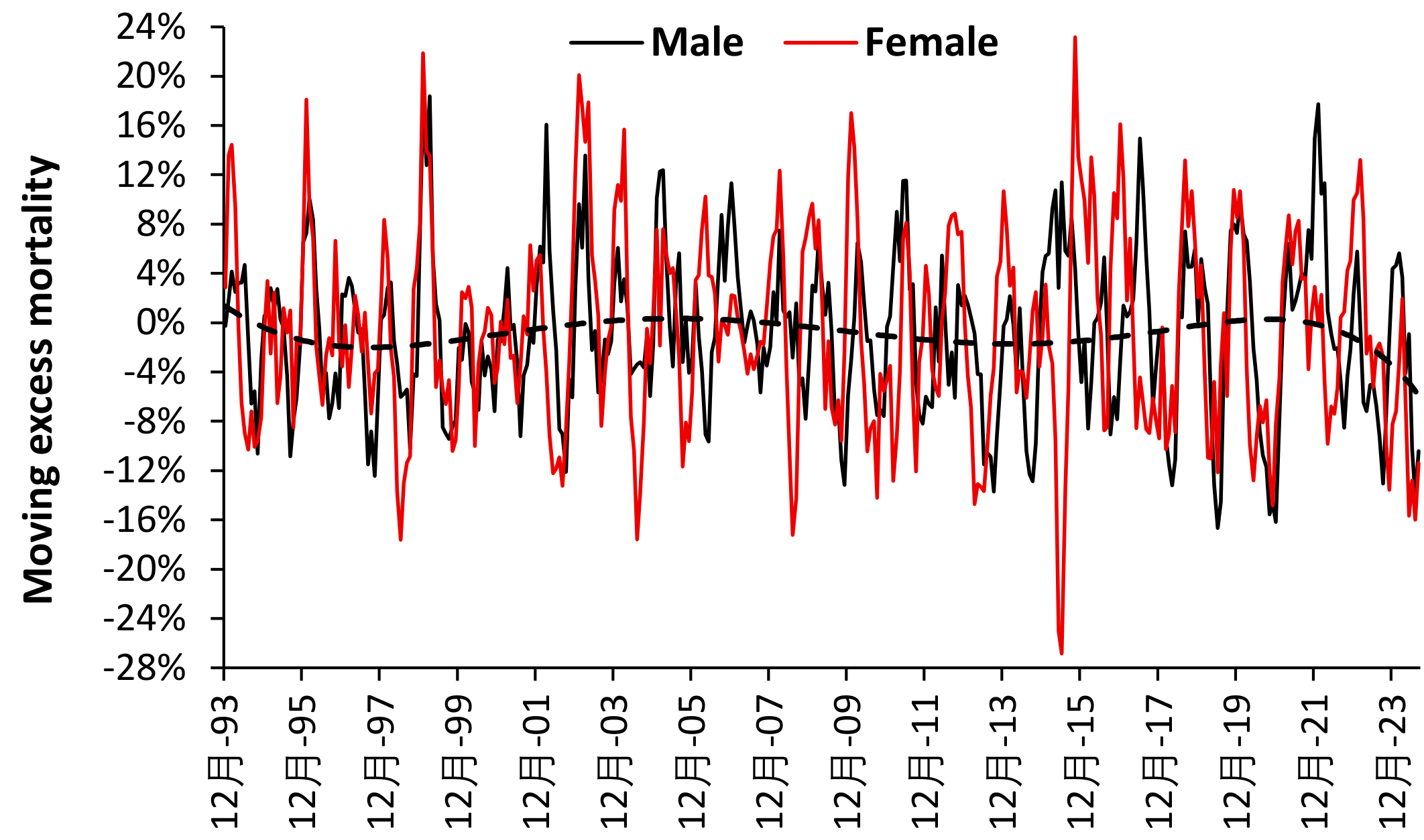
3.8. Potential Roles for Pathogens in Neonatal Morbidity

Regarding the issue of potential roles for pathogens in neonatal morbidity, Figure 11 uses a moving excess mortality calculation to locate periods of unexplained higher deaths. An excess mortality calculation compares the average number of deaths in the most recent 4 months to the average for the preceding 8 months. Then move forward by 1 month and repeat the calculation. A 4-month window gives time for any agent to spread across England and Wales. The majority of deaths in the first year of life are for neonates, usually in the first week of life.

As can be seen in Figure 11 the highest period for female deaths occurred in the 4-months ending October 2015 (+23%) while for males this occurred for the 4-months ending in March 1999 (+18%). The lowest levels of excess mortality for both males and females occurred in 2000 and 2001.

For females a 4-month deficit in mortality occurred in the period ending June 2015 which did not occur in males. Major deficits in female mortality all occurred in the 4-months ending June or July.

This method has seemingly not been used to detect the impact of uncharacterized infectious outbreaks on females and males, either during the first trimester or after birth. The dotted line suggests that there may be long-term undulations in excess mortality.

There was no noticeable excess mortality during COVID-19 when pediatric admissions appeared to reduce [4]. As opposed to adult mortality there is no clear winter-only peak in deaths. Epidemics are known to have seasonal patterns [46] and a multiplicity of pathogens seem implicated.

These hidden patterns will impact on NICU bed demand and so it is highly recommended that NICU bed occupancy be followed at daily intervals for as long as each unit has data. Recall that 100% occupancy signifies too few beds relative to demand and these need to be adjusted to estimate real bed demand. The data can then be extrapolated using anticipated trends in future births, and trends in neonatal health due to maternal obesity and declining weeks since conception at which neonates are admitted.

Given this uncertainty it is advised that neonatal units be built with excess floor space to allow for unexpected disease outbreaks and trends in pre-term neonatal medicine. An expanded birth forecasting tool is available in Supplementary material S2 which requires adaptation to cover different countries/scenarios.

3.9. Seasonality in Births and the Effect of Unit Size and Staffing Profiles

Seasonal profiles are well recognized in biology and human health and are subject to metrological and social factors including major holidays [47,48,49,50,51]. The previous study [3] highlighted that births show seasonality which will immediately impact neonatal demand and pediatric demand in the first year of life.

When approaching the quantification of seasonality, it is important to realize that there are two possible approaches.

• Assume that seasonality has a fixed profile and hence calculate averages for each month. This approach is most suited to planning staff numbers by month of the year.
• Recognize that seasonality may show variability due to changes in all the contributory factors. On this occasion a moving 12-month calculation is more appropriate. This approach is most suited to determining the maximum size of the bed pool to cope with the seasonal maximum in births.

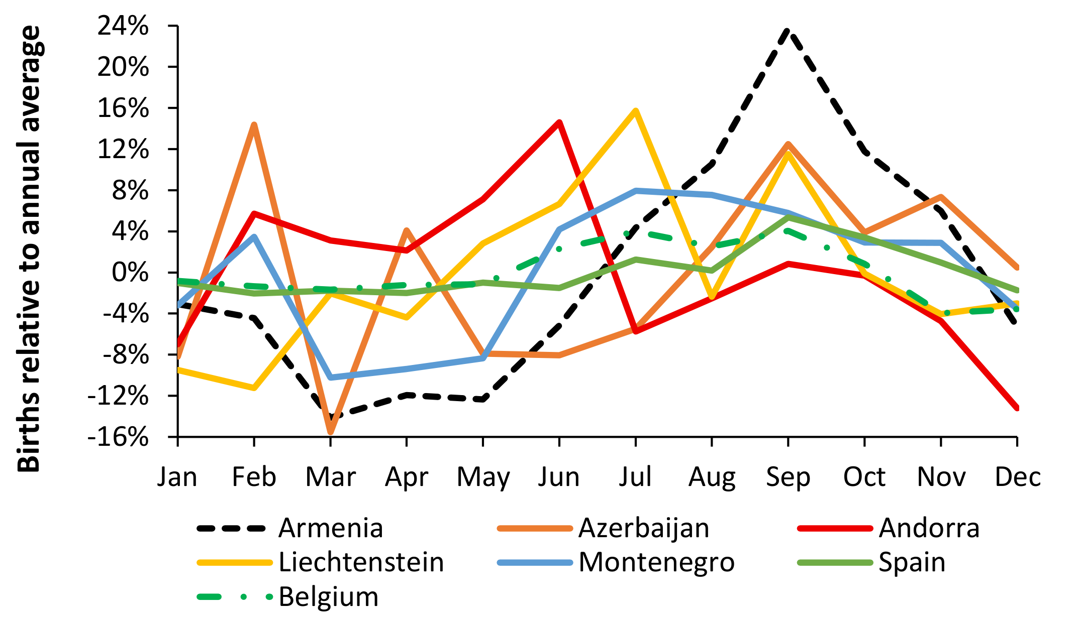
Figure 12 (using method #1) demonstrates that all European countries show unique (average) patterns in the seasonality of births and hence each neonatal/pediatric unit should be aware that the local seasonal pattern will subtly affect bed demand and staffing profiles

Note the diversity in the profiles with different months for the peak in births, different magnitudes for the peak and differences in the gap between the maximum and minimum, i.e., Armenia the largest gap and Belgium the least. Across Europe 4% of countries show the average maximum in February/July, 4% in June, 6% in July/September, 29% in July and 57% in September. The maximum in September may arise in countries with a strong Christmas/New Year holiday tradition, with December or early January being the month of conception.

Recalling that this is an average and that the maximum birth rate in every year may not always be at the seasonal maximum average month. However, for staff planning for each month this approach is appropriate.

Systematic factors are clearly involved. The key point is that the local pattern of seasonality in births must be established for each neonatal/pediatric unit, with lagged effects in the pediatric unit, i.e., seasonality in births will have a 6-month lag for admissions for 6-month-old infants, etc.

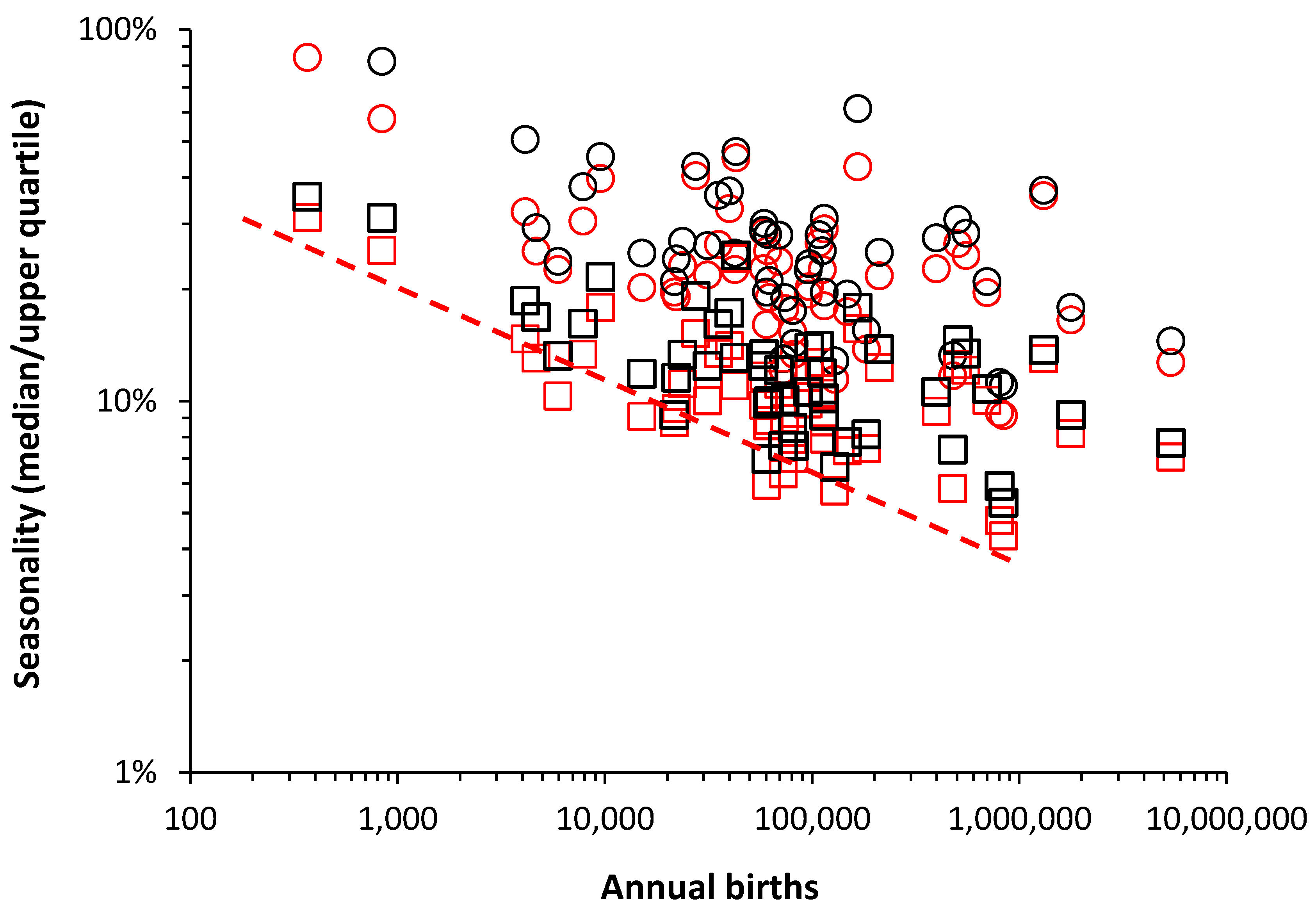
Figure 13 (using method #2) demonstrates that the apparent seasonality depends on the geographic size of the country. In Figure 13 the data at the extreme right is for the European Union. The dashed red line shows the minimum possible seasonality and a log-log decline as size increases. A more homogeneous population mix may account for some of the lower percentage increase values in some countries such as Finland, Belgium, France, etc. Countries of large geographic size such as Germany, Russian Federation and Ukraine can be expected to show region-specific profiles. At local level small number Poisson variation adds to the volatility in the seasonal profile.

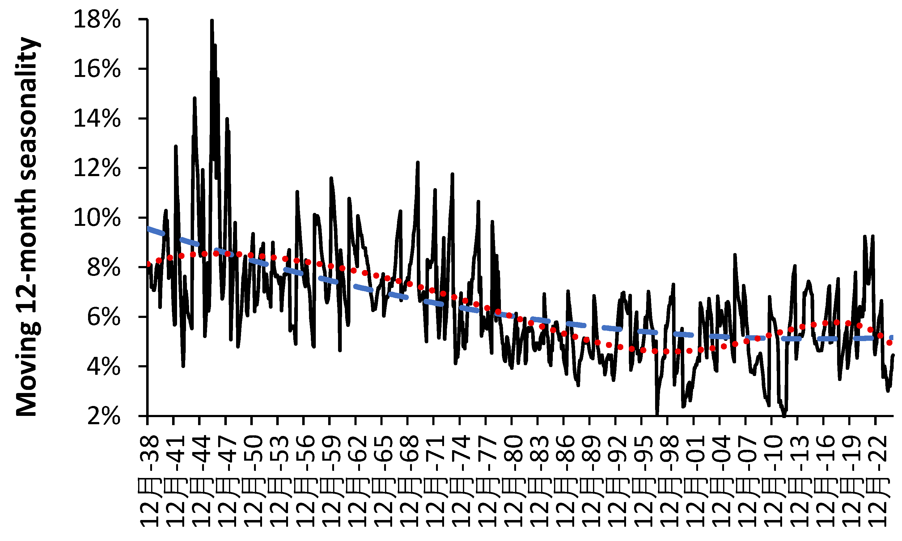
It should be noted that seasonality is not only volatile but is changing over time. For example, Figure A1 in the Appendix shows a moving 12-month seasonality calculation (maximum month versus 12-month average) in England and Wales from 1938 onward. The dashed line in Figure A1 is a polynomial curve fit. The ratios of the maximum to minimum and the maximum to the average births had the highest value of 38%/18% respectively in 1946, a local maximum of 23%/12% in 1970, and another local maximum of 21%/9% in 2021. An all-time minimum of 5%/2% occurred in 2012. More recently in 2024 there was another minimum of 7.6%/3.0% (using data from [3]). The ratio appears to decline through to the 1980s and may have reached an asymptote since then. Note that before 1978 February is the most common month for the seasonal maximum and then shifting to around July to September from the 2000s. with the 1980s and 1990s showing a transition between the two. Seasonality also seems to go through a minimum in the 1980s. Such longer-term patterns are poorly understood or investigated.

Given that births in the majority of maternity units fall below 10 000 per annum the minimum possible seasonality in Figure 12 is 10% more than the annual average at 10 000 per annum rising to 20% at 1000 births per annum.

It is suggested that for the calculation of bed numbers that the upper quartile from method #2 may be the appropriate figure to use in the two bed calculators in Supplementary material S1.

Supplementary material S4 gives a summary of the seasonality calculations for European countries between 2006 and 2015 [29]. Note how a calculation based on the average for each month relative to the calendar year average (method #1) gives a lower value for apparent seasonality than the moving 12-month method (2).

3.10. Length of Stay (LOS) and the Benchmarking Fallacy

This section is very important because there are many fallacies surrounding LOS benchmarking and the supposed reduction in costs when LOS is reduced. Detailed analysis of LOS is therefore a very important defensive step, since there is a widespread perception that LOS ‘should/ought’ to reduce ad-infinitum. While LOS did reduce somewhat rapidly during the 1970’s and 1980’s the rate of reduction dramatically reduced from the 1990’s onward [4].

In LOS benchmarking it is often insinuated that “your LOS is higher than the national average, and therefore you must be inefficient and could save x% beds by moving to the national average”. This can be called the steady state fallacy, i.e., LOS is only of primary importance in bed demand when admissions and case mix are at steady state.

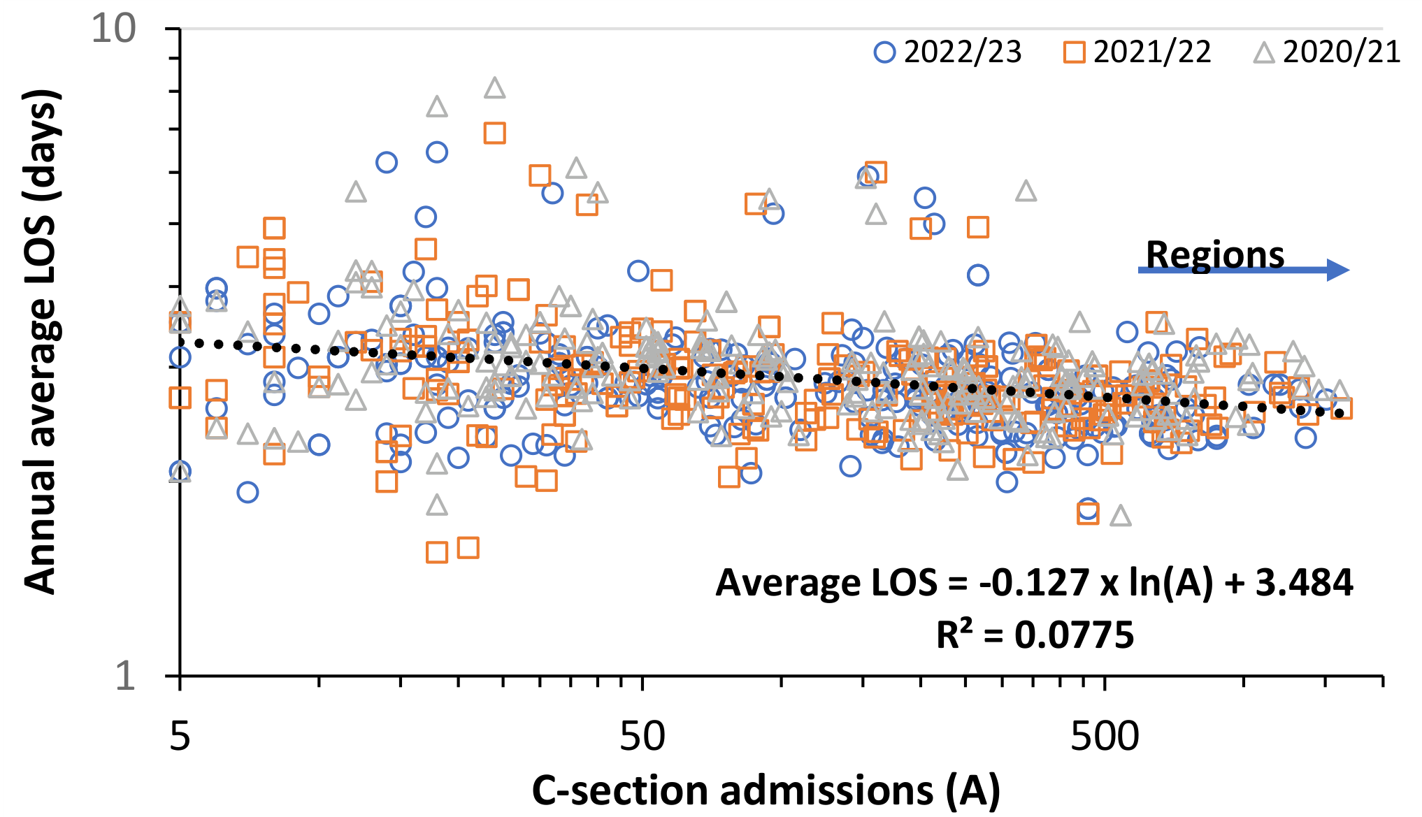
Figure 14 shows annual average admissions and avLOS for caesarian section (C-section) in Australian hospitals over three consecutive recent years, and illustrates the concept that avLOS may be unique to each hospital with its admission thresholds (private/public, size, etc), surrounding community (socio-economic, ethnic, cultural, social group, travel distance) and how these interact with government structures (health policies, health authorities, social services, etc.). This system also interacts with the meteorological and infectious environment leading to simultaneous variation in admissions and avLOS.

In Figure 14 LOS is measured at midnight and avLOS is only calculated when there are 5 or more admissions and has been truncated to remove unusually long stays. As can be seen there is a trend to higher avLOS as unit size reduces, however the dominating factor is the high annual and systematic scatter around this trend, hence the low R². The majority lie at an average below 3 days, but a subset lies at an average above 3 days.

It is my opinion that no benchmarking tool exists to adjust for the simultaneous interaction between all factors influencing avLOS. It is merely interesting but not prescriptive to attempt such comparison.

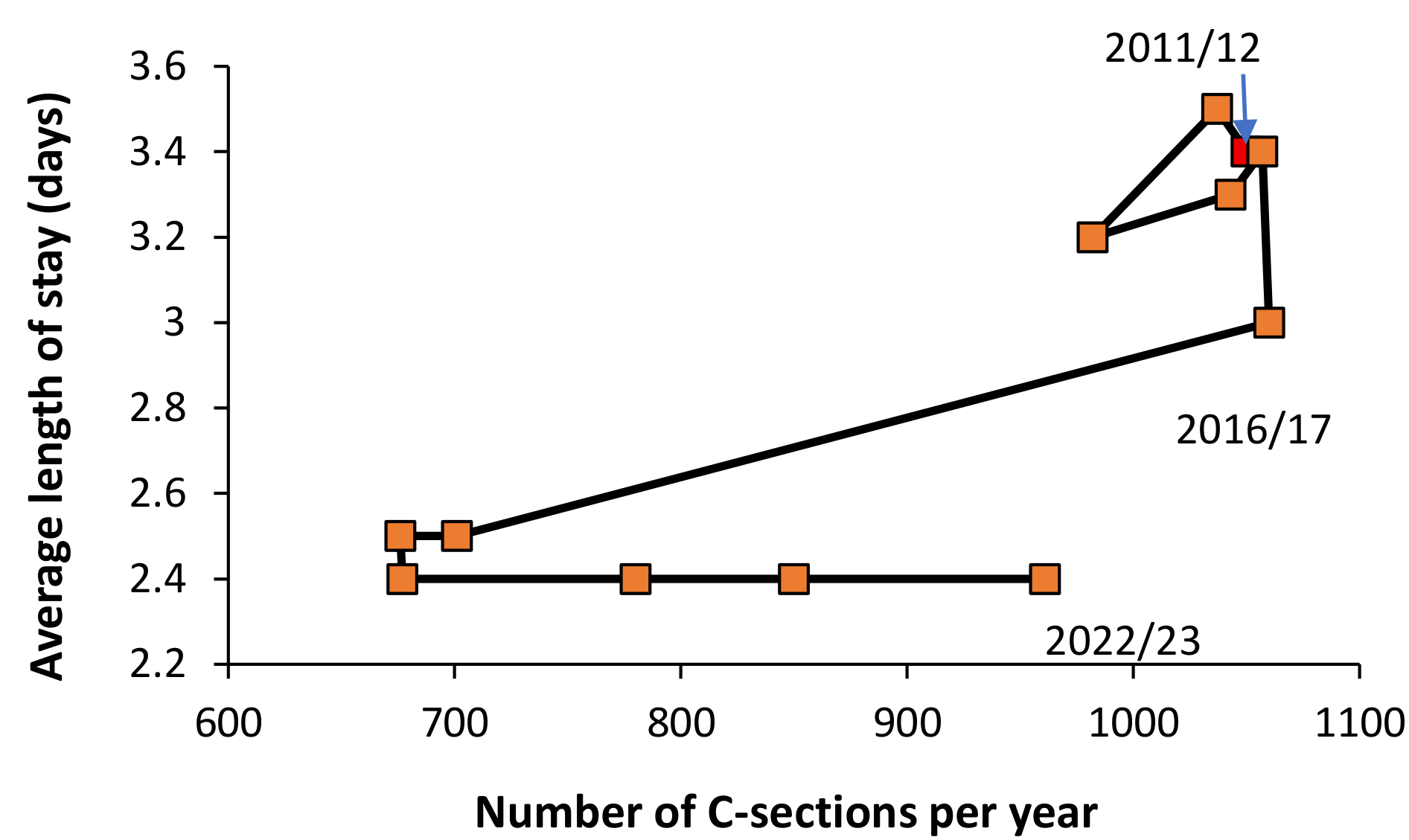
In the case of C-section, the question as to whether the procedure is clinically justified is of greater importance than arguments around avLOS. This is illustrated in Figure 15 for C-sections per year at the Mater Women’s hospital in Brisbane, Australia [37]. As can be seen prior to 2016/17 there were typically >1000 per annum at an average LOS of between 3.2 and 3.5 days stay. In 2016/17 the number of C-sections remained >1000 per year but avLOS had declined to 3.0 days, followed by massive shift to both lower avLOS and procedures per year (although the number per year has been slowly increasing since 2019/20. Note that the data in Figure 14 covers the years after the transition to a lower avLOS at this hospital.

There are several issues relating to this data.

• LOS is measured at midnight and avLOS must be calculated using real time data [3].
• It requires feedback from the mothers regarding their perception regarding the benefit of this change

If decreasing LOS is in the interest of the patient, then it should be pursued because the focus is on the patient. However, such reduction may involve changing both the hospital and surrounding social systems.

As an example, many hospitals now run ‘fit for surgery’ and ‘fit for pregnancy’ programs where patients attend managed fitness/nutritional classes to ensure optimum recovery after elective surgery or delivery. In the case of children, nutrition prior to surgery would probably be the main focus.

3.11. Unit Size and Cost per Patient

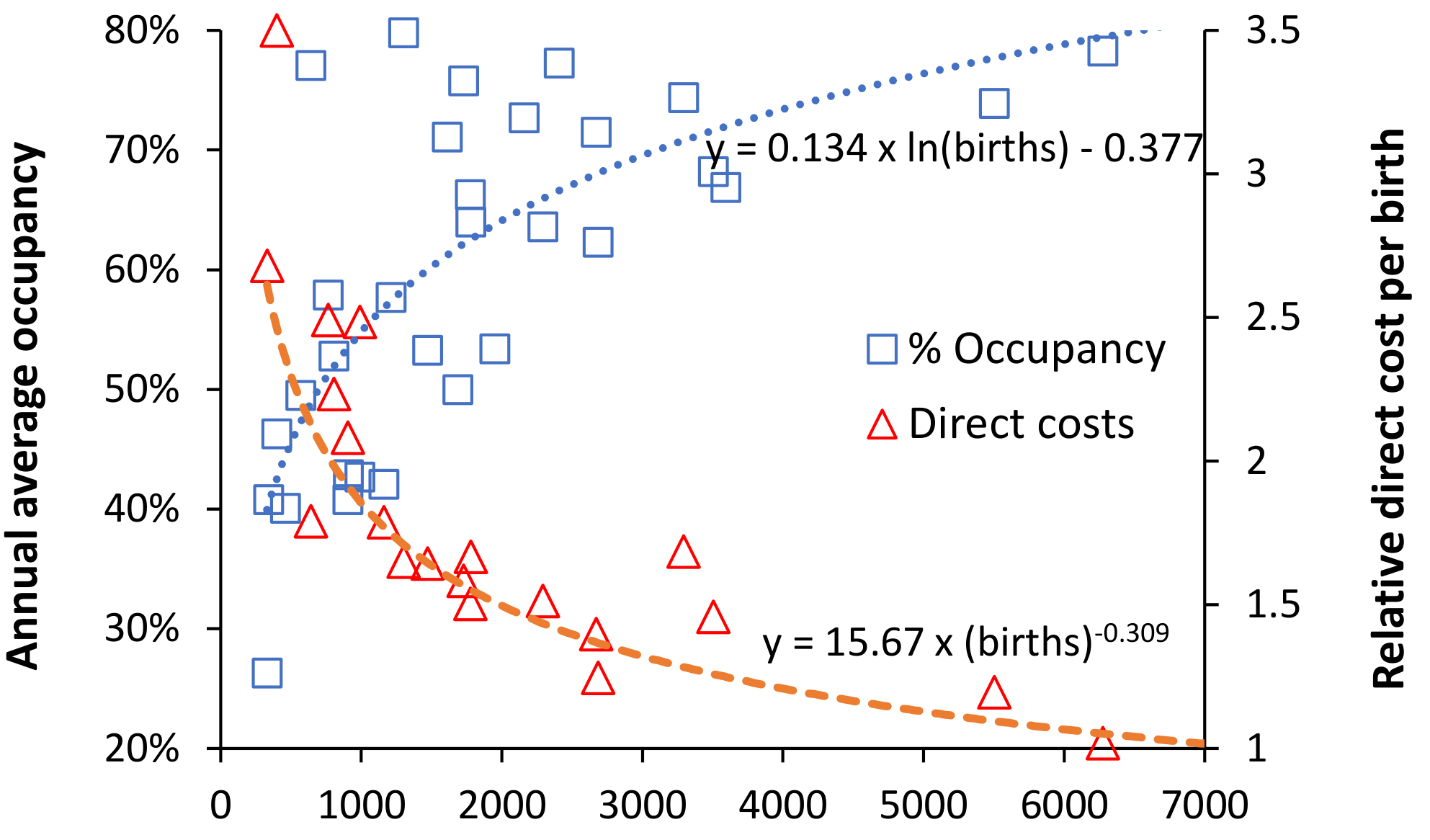
Reanalysis of the data of Thompson and Fetter [52] which covers 33 Obstetric units in Connecticut USA in the early 1960s is shown in Figure 16. Note that this study contains high scatter regarding direct costs because each of the 33 hospitals will have used different methods to allocate ‘direct’ costs. In the obstetric unit.

The trend for size and average occupancy followed Erlang B at 5.8 bed days per birth at 0.1% turn-away. Recalling that this data was in the early 1960s hence higher bed days per birth. However, the relationship between size and direct costs can be modified by running smaller units with a higher average occupancy. This only seems to occur below 3000 births per annum, i.e., where smaller size places pressure on costs, which is then compensated for by increasing average occupancy. This strategy is used in the absence of the awareness that turn-away may have deleterious consequences.

A similar situation was observed in Belgium [39,40] where some smaller units operated at large hospital equivalent bed occupancy in an attempt to mitigate the effects of small size on higher cost. In the absence of the births-to-beds calculator this behavior was considered ‘normal’. Note also that the minimum economic size estimated for Belgian maternity units of 557 births per annum [39,40] corresponds to the point where the power law relationship of size and costs rapidly escalates.

Figure 16 has excluded data from small units running at high occupancy and including this data generates a relationship between relative cost and average occupancy:

Relative direct cost = 0.942 – 1.385 x ln(average occupancy), where r-squared = 0.61

Because average occupancy is a decimal the log value is a negative and so lower average occupancy adds to the relative direct cost (as expected) while higher average occupancy is able to mostly mitigate the effect of smaller size of costs. This relationship implies that increasing average occupancy from 26% (equivalent to around 300 births p.a.) to 80% (around 7000 births p.a.) effectively reduces costs by around 45%, irrespective of size. The effect of this overriding relationship upon patient safety has never been investigated because it generates the adverse effects of turn-away.

However, the above trends were from the USA where there can often be more than one obstetric unit per town or city. The author noted that one small unit managed to operate at high average occupancy because a larger unit also operated in the same town [52]. Hence, when the smaller unit hit 100% occupancy the higher turn-away was counterbalanced by diverting patients to the larger unit. The smaller unit was effectively using the ability of the larger unit to intermittently absorb patients, leaving the small unit to run at a very competitive low cost per patient – which effectively mimicked allowing a part (say one ward) of a larger (combined) unit to operate at high occupancy. This is a ‘cunning’ but somewhat parasitic relationship.

The relevant point here is that when there is only one unit per town then smaller size looks to incur both higher capital and staff costs.

4. Discussion

The hidden complexity behind capacity planning during pregnancy, childbirth and pediatrics has been detailed using multiple sources to illustrate the multi-dimensional aspects of uncertainty and complexity. Several key points will now be discussed.

4.1. The Fundamental Role of the Trends in Births

The previous study discussed the uncertainty surrounding birth forecasts [3] and highlighted that such forecasts, especially those using the total fertility rate (TFR) methodology, were (in hindsight) extremely unreliable. Traditional fertility rate-based forecasts, as for the USA in Figure 6, typically appear to underestimate the future and lead to forecasts which are overly smoothed, compared to the more peaked behavior seen previously. Three-parameter models have been shown to give a flexible range of more realistic forecasts [53,54,55,56,57,58,59]. Unfortunately, such models require assistance from government statistical agencies who may be unwilling to assist – perhaps not wanting to challenge their TFR-based forecasts.

Uncertain/unreliable birth forecasts then invalidate subsequent maternity, pediatric and neonate population forecasts. The pragmatic and simple methods given in [3] and Supplementary material S2 allow any unit to construct alternative scenarios for future births and maternity/pediatric demand.

The whole idea is to derive a set of realistic forecasts which tend to focus on the maximum to the above average cases. The best way to prepare such forecasts is to use a moving 12-month total using historic data. Then add the alternative forecasts and compare these with the emerging actual trend. Plans are made (with flexibility) based on the alternatives. The actual births are then compared to the forecasts to derive the best-case scenario just prior to commencing any construction or refurbishment and flexibility is deliberately incorporated into any physical space so constructed.

4.2. Seasonality and Circadian Patterns

It is known that the seasonality of births varies according to the mother’s age, education, social group, parity and geography, plus additional factors [46,47,48,49,50,51]. Figure 12 [33] shows that the profile across the year for births differs by country, while Figure 13 demonstrates that the seasonal maximum in each country shows different timing and magnitude. The USA may realistically be considered as a collection of 52 countries. This suggests that the seasonality profile may be specific to each pediatric unit and this needs to be confirmed. Analysis of births in England and Wales demonstrated that the seasonality of births shows long-term trends with associated high volatility. Volatility in any form drives the real-world bed occupancy margin [2].

Seasonality in births, or more correctly seasonality in conception [48], is clearly more important for neonatal demand profiles, but will also impact pediatric demand during the first year of life as a delayed time cascade.

This form of seasonality will then interact with other factors such as temperature, pollution, weather types, infectious outbreaks, etc. [43,44,45,46,47,48,49,50,51], all affecting those of different ages to different degrees. Once again this suggests that the actual profile of bed demand will vary by location and needs to be confirmed using actual data.

It is of interest to note from Figure 12 that Belgium has numerous small maternity units, however, the relatively flat seasonal profile for this country partly mitigates against the small size of the units [39,40]. From Figure A1 the calculation of seasonality should be restricted to recent data from 2000 onward.

Regarding the circadian cycle for births, research over many years has shown a peak in normal spontaneous delivery after midnight and around 2 am to 5 am, although induction of birth has altered this pattern to between 8 am and 4 pm [60] and days reflecting clinical convenience [61]. Levels of induction may indicate resource constraints.

4.3. Unit Size (Beds), Occupancy and Turn-Away

These issues have been previously discussed in greater detail [2,3], however, the Erlang B formula has been widely applied over many years to determine adequate bed numbers [6,7,8,9,10,11,12,13,14,15,16,17,18,19,20]. The surprising thing is that government health departments fail to use it as a capacity/quality/safety measure.

Figure 2 gives the occupancy at 6 a.m. while occupancy is often measured at midnight. As pointed out by Riahi et al. [62] bed occupancy also varies by day of week, and time of day such that hourly occupancy becomes a part of genuine capacity planning.

Hence Erlang B is good enough to provide clarity, to conduct what-if scenarios and to ask awkward questions such as why does our unit operate at such higher turn-away compared to everyone else? [2,3,4].

An excellent example of the effect of turn-away comes from a study on waiting time in the pediatric ED, often called access blocking [63]. In a 347 pediatric bed tertiary hospital (whole hospital average occupancy of 68% at 0.1% turn-away) when inpatient pediatric occupancy was at or more than 80%, every 5% increase in hospital occupancy was associated with an increase in length of stay of 18 minutes for discharged patients and 34 minutes for admitted patients. With a 5% increase in inpatient occupancy, there was an increase in the odds of either a patient leaving without being seen OR = 1.21 or being treated in a hallway bed, OR = 1.18. Unfortunately, this author was unaware of the calculation of turn-away.

Another study involving 116,235 pediatric admissions for 19 common conditions in hospitals across the states of Pennsylvania and New York showed that admission day occupancy (crowding) in the pediatric units affected the LOS for less complex conditions [64]. On this occasion percent occupancy is used as a proxy measure for busyness.

Further to the deleterious consequences of turn-away, a 2013 National Audit Office (64) report conducted during the 2012 peak in births in England showed that 12% of maternity units were capping annual total births, while in the period April to September 2012 some 28% were closed to admission for more than 12 hours, with an average closure of 3 days. Some 11% were closed to admission for >14 days [65]. Considerable delays to admission will have occurred as mothers are diverted to alternative maternity sites.

The key concept from Figure 3 is to compare your unit with other units using the lines of turn-away to illustrate higher chaos as turn-away increases. An adequately resourced unit will have an annual average occupancy rate consistent with around 0.1% turn-away or lower. However, as explained previously [2,3,4] for something like a children’s hospital with a high level of elective surgery it may be possible to operate at 3% turn-away if there is a considerable amount of ‘routine’ surgery which is not overly time-critical. The same applies to critical care units, which can become the rate limiting step even for emergency/urgent surgery.

Using the births-to-beds calculator from this study it has been estimated that around 107 English maternity units had too few beds at the peak in births in 2012, or the recent minimum births in 2025. Of these 54 to 63 failed in one or more quarters around 2012 and 41 to 48 failed around 224. Of these, 13 units failed the 0.1% turn-away test in all 6 quarters [66]. Nothing was done to remedy the situation after the 2013 NAO report leading to units failing to have sufficient capacity at the minimum in births around 2024/2025.

The suggested closure of the 17 smallest maternity units in Belgium [39,40] would represent an ideal application of the births-to-beds model as it would enable managers in the ring of hospitals surrounding each of the smallest units to calculate if the additional births at their unit would necessitate additional resources (beds/staff).

Supplementary material S1 also includes a births-to-beds calculator at 3% turn-away. This is because small maternity units tend to operate above the 0.1% turn-away line. This is probably driven by financial necessity, however, 3% turn-away is probably the maximum recommended. Up to the present there has been no research regarding the interplay between staffing ratios and turn-away and the risk of adverse outcomes. The suspicion is that staffing takes precedence, because on many occasions a healthy baby and mother can be discharged early if a bed is needed. However, in the labor/birthing unit closer to 0.1% turn-away would seem sensible.

As a final comment, Erlang B assumes a constant average arrival rate, hence, it needs to be applied relative to the arrival rate for the different seasons/periods as in Figure 11. Most neonatal units simply cannot have enough beds to achieve 0.1% turn away at the infrequent points of maximum demand which may occur during an infectious outbreak. The huge spread in occupancy and turn-away in English units is symptomatic of a poor planning process [2,3,4].

The most pragmatic solution is to look at the daily arrival rate (as admissions, not discharges) over many years and attempt to be at a high occupancy level, perhaps close to 100%, during those infrequent high events. This is a risk assessment judgement which balances the capital costs of the floor space and physical equipment against the frequency of such events. This also raises the issue of how do you staff a unit in the face of volatile demand? But first, we need to understand the definition of a small unit.

Regarding the size of maternity units in the USA supposedly commencing at 1 birth [21] it should be noted that rural areas of the US without access to an Obstetric unit have increased levels of births in community hospitals without birth facilities [67,68].

4.4. Poisson Variation Is a Hard Taskmaster Especially to the Small Unit

It has been observed by DeSisto et al. [25] that in the USA the size for a maternity unit commences at a nominal 1 bed and that 55% of maternity units handle fewer than 1000 births per annum. So how do we define a small unit? Poisson statistics describe the variation around the average for integer events (patients) relating to their average daily arrival rate. It has been used extensively for over 100 years in epidemiology and capacity planning [6,7,8,9,10,11,12,13,14,15,16,17,18,19,20]. At high numbers (generally >100 per unit of time) it can be approximated by a normal distribution but at smaller rates there is an increasingly skewed distribution. While the standard deviation is always equal to the square root of the average arrival rate, there is a minimum of 0, the average and the average minus 1 are the most common arrivals, and to compensate for the minimum of 0 there is a tail of higher arrivals possible per unit of time.

How does this dictate the definition of a small unit? At an (assumed constant) average of 8 arrivals per day, one standard deviation (STDEV) is equal to 8 ± 2.83 arrivals such that 0 or 1 arrival occurs about once a year, as do 16+ arrivals. Both 7 and 8 arrivals occur on around 51 days each per year. If the avLOS is 2 days (calculated at midnight) there will be an annual average of 16 occupied beds, and at an average occupancy rate of 80% (a high figure), the unit has 20 beds. What do you do on that 1 day when 16 patients arrive, and you have 16 occupied beds? You can immediately admit the 4 most acute patients and the 12 must wait in a queue (with triage). You can possibly arrange a hasty discharge for 8 patients, leaving 4 still waiting.

Hence the reasoning is that 8 arrivals per day (around 3000 births per annum) represent a small unit, which lies at the upper quartile of units in the USA [25], i.e., 75% of US maternity units are small to very small. This illustrates the importance of size and the lines of immediate turn-away in Figure 3. The USA has far lower population density than England and this is a common problem for many countries such as Australia, large parts of Africa and even the rural parts of India and China. The result is that capacity planning in most US maternity units is dominated by Poisson-based chance variation in admissions.

The study of DeSisto et al. [25] shows that 20% of births in the US occur in maternity units with <700 births per annum, while 80% of US maternity units have fewer than 2000 births per annum. Units with >7000 births per annum only account for 1.2% of hospitals. The above definition of 8 per day, i.e., around 3000 births per annum places around 90% of US births in small to tiny units. Figure 5 demonstrated a similar picture for pediatric units in the USA while Kozhimannil et al. [67,68] associate higher adverse outcomes with small maternity units and the same would be expected for smaller pediatric units.

Monte Carlo simulation and other operational research tools which will partly rely on Poisson statistics and Erlangs equations can therefore be employed to examine whether staffing and bed occupancy benchmarks are likely to work in the real world [69].

One study in Belgium where (for historic reasons) there is an abundance of small hospitals suggested that the minimum economy of scale occurred at 557 births p.a. [40]. Similar calculations were conducted in a 1963 [52] study based on US maternity units, as shown in Figure 16.

The situation in the USA is further compounded by the operation of a ‘free market’, some may call it a free-for-all, where hospital chains compete for market share resulting in multiple hospitals in each city/town where a system of rational planning would only have one larger hospital with consequent lower costs per patient.

4.5. Benchmarking avLOS

Before discussing avLOS, it is important to dispel misunderstanding regarding its role in bed demand. In elective/scheduled care it is absolutely true that reducing avLOS reduces bed demand and increases throughput per bed and therefore reduces the capital cost per patient and increases income per bed. Hence, implement a full range of patient-centered strategies to achieve this aim. While such strategies can also be applied to emergency/unscheduled care they have less impact on bed demand because it is the volatility in admissions and seasonality which sets the required number of beds and their average occupancy. Reducing avLOS is thus appropriate for all the elective/scheduled aspects of wider adult care. Since maternity and pediatrics are mostly emergency/unscheduled care the capacity planning process requires different thinking.

Interestingly from 1998/99 onward the number of occupied beds in the NHS stayed approximately constant, leading to escalating bed occupancies as the supply of beds declined as the PFI hospitals replaced the previous old hospital buildings [1,2,3,4]. This then created a somewhat obsessive need to decrease LOS by employing aggressive LOS benchmarking between hospitals. The lowest LOS was always declared to be the best/optimum LOS. The problem is that this type of benchmarking can lose sight of what is best for the patient – within a wider social context for children or mother/baby in maternity.

Figure 14 used Australian data for C-section to show high variation between units of similar size but in different parts of Australia. Any benchmarking requires far greater understanding of the complex contribution from societal, social group, distance, size and pressure on units with too few total beds.

4.6. The Illusionary Effect of LOS on Costs

Having established that the primary driver for bed occupancy is the volatility in admissions, it is apposite to investigate some of the myths surrounding LOS and costs [70,71,72,73,74,75,76]. Logically, any disease/procedure dictating an extended stay will have a higher cost, however, this does not automatically mean that reducing LOS will make a significant reduction in cost. In 1970 Lave and Lave [73] pointed out methodological difficulties and pitfalls for costing in a multiproduct setting such as a hospital. These have likely been ignored in the rush to demonstrate large savings. There are numerous studies claiming large reductions in cost by reducing LOS. However, the suspicion is that most of these studies have made erroneous assumptions around the behavior of costs in the real world.

Firstly, most studies are conducted in large hospitals which allows for higher average bed occupancy and diminishes Poisson randomness. Hence the hidden assumption is that costs in smaller hospitals behave the same way as in larger hospitals. This has never been investigated.

Perhaps one of the most important studies demonstrated that the cost elasticity for the effect of reducing avLOS on costs in the USA was very low, falling in the range 0.09-0.12. It shows that common perceptions regarding the extent of cost savings resulting from LOS reductions have been substantially overestimated [74].

Another erroneous assumption is that the cost per day is the average for the entire stay [75,76,77]. The daily cost typically shows an exponential decay with time [76]. One study demonstrated that the last full day of hospital stay for 12 365 surgical patients accounted for only 2.4% of total costs [75]. For patients without a major operation the last day accounted for 3.4% of costs, while those with a LOS of 4 days the last day accounted for a slightly higher 6.8% of total costs [75]. The authors stated that “physicians and administrators must deemphasize LOS and focus instead on process changes that better use capacity and alter care delivery during the early stages of admission, when resource consumption is most intense”.

This fallacy is further exposed in a study relating to CCU costs which showed that the first day accounted for 67% of total direct costs. Daily costs had declined to 40% of the average on the fifth day [77]. It is unsurprising that reducing LOS does not yield the anticipated benefits promised by simplistic cost assumptions.

An additional fallacy is to assume that fixed costs are variable. A US study calculated that 84% of hospital costs were fixed. Of this 32% were for support functions such as utilities, employee benefits, and housekeeping salaries, while 52% included direct costs of salary for service center personnel [78].

It is sometimes forgotten that to reduce LOS involves more intense input into the earlier days of the stay which can counterbalance and cost savings from decreasing the later less intensive days [79]. Hirani et al. [80] suggest that the cost of follow-up care may sometimes unexpectedly increase or have been omitted from the cost calculations. Indeed, identifying a problem while mother and baby are still in the maternity ward can avert a more serious readmission from the community [3].

Bowers et al. [81] point out several issues, namely that you cannot reduce staffing in proportion to a reduction in avLOS, that reducing avLOS increases the intensity of nursing care per patient, and that community resources have to be expanded to cope. The net cost saving is uncertain.

Lastly, in the study of Baretta [82] recommended that ‘indirect’ costs should be excluded from benchmarking studies because their inclusion led to serious errors in the determination of cost ‘efficiency. This issue is covered in the next section.

4.6.1. The Fixed (Indirect) Costs Dilemma

The greatest fallacy around LOS lies in ‘the fixed costs dilemma’ [3], where up to 60% of the cost of admission arises from the fixed (sometimes called indirect) costs of shared hospital supporting departments such as the hospital board of directors, finance, human resources, press and PR, etc., and depreciation on capital assets (buildings and equipment), etc. Note that the figure of 60% applies to the USA where private healthcare imposes high transaction costs on hospitals such as excessive documentation of every cost item, individual invoices for every patient, offering payment plans to those who are uninsured, debt collection, etc. This proportion will be lower in other countries. Such fixed costs never go away but can be partly mitigated by economy of scale for the non-patient facing departments [83].

The fallacy lies in how these costs are shared (apportioned) with the total cost assigned to the patients. The moment that these fixed costs are apportioned based on LOS, then LOS suddenly becomes ‘expensive’. The correct way to share most fixed costs is based on admissions rather than LOS. This is a logical basis since the first day of the stay is the most expensive (as shown above) and the administrative costs occur at admission/discharge. As a simple example, a hospital has $10 million in fixed costs with 10,000 admissions and 50,000 bed days. Apportionment based on admissions adds $1,000 to each patient while on LOS adds $200 per bed day. If LOS is reduced by 1 day per patient, the fixed cost per day simply rises to $250 per bed day. As soon as the shared overhead costs are allocated by admission it becomes far clearer that the route to reducing costs may have more to do with administrative costs and the cost of capital (buildings, etc.) which becomes excessive in small hospitals, than in the direct medical costs.

A similar logic applies to ED and outpatient attendances, namely, allocate the fixed costs per attendance and not based on the length of the consultation, although with additional modification for complexity.

In addition, every department has largely semi-fixed costs for staffing, which stays roughly the same independent of how admissions may fluctuate [78]. Hence, if admissions are 15% lower or higher in one year, frantically seeking to reduce LOS will have virtually zero effect on total staff costs.

Regarding fixed costs for staffing, studies in England have shown that the average nursing cost per occupied bed day reached a minimum around 35 average occupied beds and was 3-times higher at 10 average occupied beds. The relationship was exponential with size {84]. Another study showed that a 5-bed unit had 4-times higher costs per bed than a 35-bed unit. Costs rapidly escalated exponentially below 15 beds [85]. These results confirm the strong diseconomy of scale noted in Table 1. An optimum unit size of around 30 beds is also noted in the next section.

The previous study on maternity capacity highlighted that dubious cost assumptions are often involved in justifying shifting postnatal work into the community [3]. The maternity/pediatric department must question any source of advice claiming that reducing LOS will make substantial savings.

4.6.2. Economy of Scale and the Cost per Patient

Economy of scale (EOS) is a well-recognized concept which has a defining impact upon the cost per patient [86]. Freeman et al. observe that EOS is stronger for unscheduled care [87]. A 1993 study by Perkins [88] details research on EOS in obstetric care going back to the 1930s. EOS was shown to be highly relevant to the Belgian system of obstetric care via a multitude of small hospitals [39,40]. A minimum economic EOS in obstetric care was observed at 557 birth p.a. with increasing EOS up to at least 900 births p.a. [39,40]. Seemingly little has changed since the 1930s [88].

It should come as no surprise to find that US hospitals which invest heavily in capital (buildings/equipment) to increase market share end up with inflated costs arising from the higher costs of capital depreciation and running costs per patient [89].

At the whole hospital level studies show that below 200-300 beds there is diseconomy of scale, and the total cost per patient shows economy of scale above 200-300 beds and reverts back to diseconomy of scale above 600 beds [86]. The increase above 600 beds probably arises from the fact that larger hospitals can offer increasing specialization and treat the most complex cases. As a reference point, in England maternity comprises around 7% of acute hospital beds [90]. This ratio implies an optimum size of 32 maternity beds and an economic minimum size of 14 beds.

In Belgium where the minimum economic size for a maternity unit was evaluated to be 557 deliveries per year [39,40] it was noted that 17 small units (15% of units) could be closed while still maintaining a 30-minute drive time [39]. In the USA 557 deliveries would exclude 35% of small hospitals with more than 25 births per annum [25], however drive times remain an issue since only 61% of the population are within 30 minutes of obstetric care, while only 33% have 30-minute access to level 3 neonatal care [91]. By way of contrast, in England 79% of mothers live within a 30-minute drive time and 99% are within 60 minutes. Only 8% have no Obstetric unit within 30 minutes [65].

This does not mean that reducing LOS via new technology/medications or optimum care pathways is not helpful. As Taheri et al. observed [71] it is far better to focus elsewhere and this will include issues around how to avoid clinically unnecessary admission and/or intervention [92,93,94,95,96], or how best to provide non-admission-based care which saves real costs [97].

The issue here is that small units are unable to reduce their staffing costs because there is a minimum staffing level simply required to run a ward/unit [84,85]. This is a fixed cost set against a highly variable daily number of admissions (as per Section 4.4) and bed occupancy. Attempting to reduce avLOS to reduce costs is futile, although still encouraged provided it benefits the patient.

4.6.2. HRG/DRG Tariffs, Fair Costs and Long-Stay Patients

While the reality exists that most hospital costs behave as if they were fixed [78], uninsured patients, insurance companies, and governments all demand that they be presented with a ‘fair’ price. Most of these ‘purchasers’ believe that staying longer costs more – hence the push to reduce LOS. While I have indicated that many costs can be apportioned based on a count of admissions a more nuanced approach is required.

Length of stay could be argued as being related to certain direct costs such as catering, laundry of linen, consumables, and the depreciation costs associated with the bed, ward equipment and floorspace. These will not account for a large cost per day stay. Recall that costs decline in an approximate exponential decay as time since admission increases [76].

Staff costs become more problematic and should probably be split between the counts of admissions and total bed days. However, recall that occupied bed days depends on admission and admissions are subject to both Poisson and environmental variation. You only know the total at the end of each financial year, which suggests that you need to estimate the minimum number of admissions and occupied bed days for each year. To assume an average is to invite financial disaster.

In 2004 I conducted a large Monte Carlo simulation to see how income would vary based only upon Poisson variation associated with an assumed average number of elective admissions into each of the available elective HRG/DRGs with their unique prices for payment to the hospital [98]. This was for a medium/large English hospital with 670 beds (large/very large by US standards), with an expected 31 200 elective admissions at a present-day elective income around £63 million (multiply this by 2 to get a $US equivalent). This best-case simulation gave around a £5 million range in income (£60.4 to £65.2 million) and a 1500 range in elective admissions (30 400 to 31 900). In the real-world elective admissions have 2 times higher variation than Poisson statistics while emergency admissions are 3-times higher than Poisson. Hence, the range in income doubles from £5 million to £10 million, etc. Clearly the inclusion of emergency admissions would give a greater range in income and admissions. As an aside, note that the probability distribution for income versus admissions is shaped like a tilted ellipse with sectors like low admissions/low income having a higher probability than low admissions/high income, etc.

The dilemma is obvious, with largely fixed costs having to be met by variable income, and actual costs needing to be allocated against variable admissions, while simultaneously needing to deliver the surplus/profit required for the purchase of new equipment and other capital investment. That which may at first seem simple is profoundly complex. Made more complex when the HRG/DRG tariff makes no allowance for economy of scale.

It is suggested that the obstetric/pediatric departments have a discussion with their finance department around the proportion of their price which is due to overhed costs and the alternative ways in which prices could be calculated, compared to what purchasers are willing to pay – all part of any decision regarding new investment to cope with rising demand or disinvestment.

4.7. Is Deprivation the Main Driver of Obstetric/Pediatric Excvess Bed Demand?

Deprivation is commonly used as an explanatory variable for excess bed demand. However, my own (un)published research shows that social groups rather than deprivation give far greater predictive power. Social groups reflect health behaviors while deprivation does not primarily do this [99]. Social groups are often constructed using the same methods to construct consumer groups. The maternity study [3] demonstrated how the trends in births in England profoundly depend on social group. Social group is highly likely to reflect population density (in the next paragraph} and will also reflect risk factors such as obesity, etc.

A study regarding demand for ambulance services among children and the elderly showed that population density, not deprivation per se, was the primary determinant for the call-out rate. Deprivation showed a very weak linear relationship while population density had a strong non-linear effect with a sharp decline in call-out rates below 1000 persons/km² (2600 persons per square mile) dropping to near zero rates in lowest population density areas [100].

A recent study suggested that age standardized mortality rate (ASMR) in children may be an additional relevant factor [2,4]. On this occasion ASMR is an alternate measure of the experienced ‘deprivation’ in relation to health. Further research is required on the social and other factors influencing bed demand in both obstetrics and pediatrics.

4.8. Year of Birth Cohorts and the Forecasting Spreadsheet

It is almost an industry standard to use 5-year age bands in capacity planning. No one questions this but simply follows the crowd. The cyclic behavior of births seen in many countries shown in Figure 5 and Figure 6 implies that every 5-year age band will be subject to waves of births passing through the age band which will interfere with the outputs based on this method.

The forecasting spreadsheet in Supplementary materials S3 invites the reader to follow the admissions/occupied bed days for year-of-birth cohorts up to 19 years after birth. This approach seeks to direct analysis away from simplistic use of wider age bands in capacity planning. Each birth cohort lies in a diagonal across the spreadsheet.

This is based on the recognition that birth cohorts can have lifelong patterns of health. For example, birth during different parts of the solar cycle seem to influence longevity and disposition to certain physical and mental conditions [101]. Exposure to antibiotics and pathogens during prenatal and early life can influence health trajectories across the lifespan [102], and H1 influenza exposed cohorts look to have worse health outcomes than H3 exposed cohorts [103].

Outside of the first 19 years of life, the WW II baby boom in England led to 1.8 million births between May 1946 to May 1948 which was 50% higher than the point of minimum births between November 1939 and November 1941. In 2025 this birth cohort was aged 79 to 81 years and represents a sudden onset of increased healthcare demand which moves forward in time. Indeed this cohort began to appreciably affect inpatient demand around 2011 when they were 71 to 73 years old.

These combined factors are called age-period-cohort (APC) effects and influence the health response to the environment experienced in the current year. They are difficult to disentangle [104] but nevertheless are yet another source of variability/uncertainty regarding each year’s level of admissions and bed demand. Birth cohorts remain an area of international interest [105] and form part of the evolving patterns of volatile bed demand

The forecasting spreadsheet S3 simply gives the opportunity to see the outworking of the APC effects using local data and reinforces the futility of using averages in demand/bed capacity forecasting.

All APC models appear to focus on the babies and their life course and I am not aware of any APC studies investigating the mothers and the complications associated with pregnancy and the effect on the babies at birth.

5. Limitations of the Study

Births are used as the closest approximation to women falling pregnant because data on births is widely available.

Note that annual births, monthly seasonality and bed days per birth are all subject to statistical, environmental and infectious forces, hence the need to operate with a slight excess of beds. This excess can be investigated using the bed calculators provided in the Supplementary material S1.

Hence, the study recommends that capacity planning leaves room for flexibility in the building design to cope with unexpected changes in demand. All manners of financial, staffing and other issues will impact this imprecise ‘risk’ evaluation.

6. Key Recommendations

Several key recommendations arise from this study.

• Although the USA and UK have some of the most extreme examples of cyclic birth trends this does not imply that all areas within these countries will follow the same patterns [3]. Health departments should insist that statistical agencies prepare a wider range of birth forecasts which can include those based on TFR, three-parameter models, and other pragmatic local approaches detailed in this and the previous study [3]. They must ensure that the potential range of births is communicated to all regional health authorities and hospitals. Hospitals should have contingency plans to deal with anticipated periods of higher births [3] and deal with surges in demand from seasonality.
• The ideal position is that pregnancy, childbirth, neonatal and pediatric care be free of charge and funded from hypothecated state general taxation. For-profit health insurance with its inherent high transaction costs, and temptation to maximize profits is incompatible with care delivered to those who are unable, by virtue of childhood, to earn money. The USA appears to exemplify this requirement with disturbingly poor childhood mortality across all age bands [4]
• It must be clearly understood that small maternity/neonatal/pediatric will suffer from unavoidable high capital and staff costs per admission and that these costs will be further distorted by the allocation of shared overhead costs as was discussed previously [3].
• Health Departments may need to operate maternity/pediatric units in remote locations where rationalization is not possible.
• High inpatient occupancy (and related turn-away) are known to be associated with delays to admission and poor patient outcomes such as hospital acquired infection rates [2,62,106]. Such studies are usually conducted at large units where bed occupancy is used as an (incorrect) proxy for turn-away - although the bed occupancy rate is also a proxy measure for busyness. An upper limit on turn-away should be stipulated. Given the fact that many units operate at an annual or quarterly turn-away less than 0.1%, it is suggested that no unit should operate at >5% turn-away in the worst month.
• Bed demand is highly seasonal with occasional high years. The bed planning calculation is therefore one regarding available floor space rather than a fixed number of beds. The floor space simply provides the opportunity to flex the number of available beds. Such flexibility is profoundly important for staffing, which dictates against small units. It is recognized that units situated in small towns and remote areas will struggle to implement such flexibility unless on-call staff can be redeployed from elsewhere.
• The inherent volatility in neonatal bed demand implies that the actual trends in occupied beds become the benchmark rather than futile attempts to separately forecast admissions and LOS – which are both part of the inherent volatility.

7. Research topics

This study highlights several key areas for future research

• The evidence seems to show that small units are structurally expensive simply due to the high Poisson randomness in arrivals. More studies are needed in this area as somewhere around 30 beds could be the optimum size.
• Is neonatal mortality highest in countries with highest proportions of small units, i.e., with less than 10 beds.
• Are units with high turn-away associated with low avLOS, i.e., low avLOS has become an indicator of poor planning rather than an efficient unit.
• The interaction between turn-away and staffing on adverse outcomes is an area in urgent need of investigation. This interaction is likely to depend on the size of the unit. Recognition needs to be given to the fact that high levels of transfers out of small hospitals will simply shift the poor outcomes to the receiving hospital.
• International data on total curative beds need to be segmented to include data on pediatric, maternity and mental health beds and occupancy. Measures of the average number of available and occupied beds are required for each country.
• A specific study is required regarding international levels of maternity and pediatric available and occupied beds.
• A simple tool should be freely available to allow hospitals to calculate their annual average and monthly levels of turn-away. The inputs are average beds available and average occupancy for any period. Ideally this could be via the WHO, World Bank, or government health department websites.
• While pathogen interference has been mostly researched for adults’ additional research is required specific to neonates and how the pathogen mix varies from year to year. Common persistent pathogens need to be considered as contributory factors.
• A review is required regarding the approaches in different countries to the issue of pediatric and maternity inpatient care for rural and remote populations. This will be influenced by relative wealth and how care is funded. See #8 below.
• Specific research is required regarding how care is funded relating to distance, unit size, and cross-border flows in Federal countries.
• A study is required to document capital, staff and overhead costs per patient relating to unit size and how to calculate equitable adjustment factors to underpin HRG/DRG payment systems.

8. Policy and Funding Implications

The effect of relative wealth on hospital bed provision was addressed in parts 1 and 2 of this series [1,2]. Maternity costs in the USA are a structural issue. In 2000 some 61% of maternity units handled fewer than 1000 births per annum, which drove closures due to cost pressures, leading to 55% of units below 1000 births in 2019 [25]. These units, mostly servicing rural/remote populations, cannot reduce their costs and a national strategy is required for optimal placement which transcends State and County borders [3].

It could also be argued that the number of units permitted in medium/large towns and cities be limited to ensure lower costs through economy of scale.

In terms of safety, small rural units have problems recruiting staff and maintaining adequate staff to patient/birth ratios during both the seasonal and the frequent times of Poisson-induced higher-than-average demand [67,68,107].

The most relevant policy implication is the funding of maternity and pediatric services via hypothecated taxation and direct payment to providers. This minimizes the futile cost burden of private health insurance and claim processing. The next is around state supervision of capacity planning to ensure equitable distribution of resources and that hospitals operate at acceptable levels of average occupancy, turn-away and safety.

9. Conclusions

This study should be read in conjunction with the associated maternity [3] and pediatric [4] capacity planning studies. The use of queuing theory and the Erlang B equation for maternity unit capacity planning was first advocated in 1959 [8], however, there appears to be widespread ignorance to its importance. Two bed calculators are provided in the supplementary material S1 which can be used for obstetric, maternity, midwife-led, birthing wards, obstetric theatre, neonatal and pediatric unit bed capacity.

Tables/calculations can be easily generated linking births and average total bed days per birth to the required number of available beds. These calculators enable the rapid testing of multiple what-if scenarios with the first calculator allowing for the input of seasonality and day of week effects to give the maximum required beds in the highest birth month and for the impact of ‘elective’ C-section and other interventions on the weekday profile. Larger units benefit from considerable economies of scale in both throughput per bed and cost per patient.

The reality of economy of scale on the unavoidable higher costs in smaller units implies that HRG/DRG tariffs must have a mechanism to avoid underfunding such units. However, such units are often forced to operate at high occupancy and turn-away to remain financially competitive with larger units irrespective of the deleterious effects. This is especially the case since countries have different maternity unit size distributions depending on rural/remote population characteristics and on historic factors. In Belgium the minimum size for a viable maternity unit has been estimated at 557 births per annum [39,40] which presents problems in countries with high proportions of rural/remote populations. This disparity also exists when there is a very large gap between the smallest and largest units. Health departments seem to have forgotten the reality of this link. It is exceedingly unwise to pay all maternity/pediatric units using the same HRG/DRG tariff and not expect to inflict significant financial and safety issues upon smaller units.

The LOS for common birth events varies greatly between countries [38], although further studies are required regarding the link between LOS and patient/baby outcomes.

Forecasting future births is highly dependent on local factors including construction of new dwellings and the availability of employment suited to young families. This area requires greater input from health departments and statistical agencies.

Neonatal bed requirements are shown to be complex, which implies that they should be built with excess floor space to allow for unexpected/unplanned future trends.

Universal funding for maternity/pediatric care is the recommended standard, however, hybrid options do exist such as the American state of New York’s ‘Basic Health Program’ [108].