Submitted:
03 January 2026
Posted:
05 January 2026
You are already at the latest version
Abstract
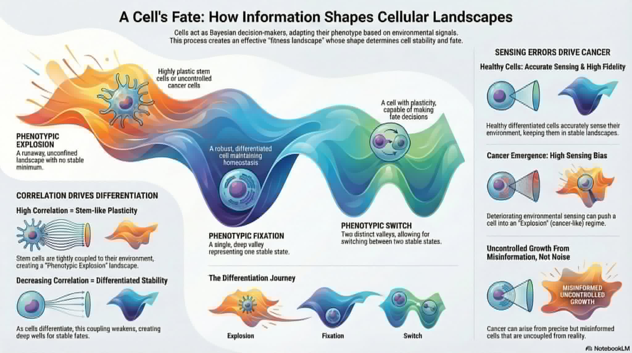
Cells adapt their phenotypes in noisy microenvironments while maintaining robust decision-making. We develop a coarse-grained theoretical framework in which cellular phenotypic adaptation is described as Bayesian decision-making coupled to replication and diffusion. This leads to an effective Fokker--Planck equation with an emergent fitness landscape governing phenotypic dynamics. We identify distinct phenotypic regimes—homeostatic fixation, bistable decision-making, critical switching, and runaway explosion—and propose a biological interpretation in which homeostatic and bistable landscapes correspond to healthy differentiated cell states, whereas explosive landscapes capture stem-like or cancer-like behaviour. In the Gaussian setting, the correlation $\rho$ between intrinsic and extrinsic states directly encodes mutual information and acts as a bifurcation parameter: high correlation produces shallow or explosive landscapes associated with phenotypic plasticity, while reduced correlation stabilises differentiated fates by deepening potential wells. We further show that proliferation reshapes these landscapes in a nontrivial manner. Proliferation conditionally may stabilises local homeostasis without altering global confinement, or cooperate with biased environmental sensing to eliminate homeostasis/bistability and drive cancer-like phenotypic explosion even at high phenotypic fidelity. Finally, we show that negative intrinsic–extrinsic correlations suppress explosive dynamics but also reduce bistable plasticity, suggesting a robustness-plasticity trade-off. Together, our results suggest that development, tissue homeostasis, and carcinogenesis can be understood as information-driven deformations of a Bayesian phenotypic fitness landscape.
Keywords:
cell decision-making
; Bayesian inference
; dynamical systems
; Fokker-Planck equation
; phenotypic dynamics
1. Introduction
Decision-making consists of identifying objectives and choosing actions that optimize outcomes among available alternatives [1]. In a similar spirit, cells can be regarded as decision-making agents that adapt their behaviour through phenotypic evolution in response to local micro-environmental cues, while operating under fixed intrinsic regulatory wiring. Cells sense information from extrinsic variables such as ligands, nutrients, cell density, or mechanical stress, which is encoded into internal states via biophysical and biochemical processes. This information is subsequently decoded into phenotypic responses, creating a feedback loop in which cellular decisions reshape the microenvironment [2,3,4,5,6].
A defining characteristic of cellular decision-making is its stochastic nature. Cells operate in noisy environments and experience fluctuations arising from low copy numbers of molecular species, environmental variability, and intrinsic stochasticity in biochemical reactions [7]. Noise is not purely detrimental; it can play a constructive role in probabilistic decision-making, generate phenotypic heterogeneity, and support bet-hedging strategies [8,9,10]. The filtering, amplification, and utilization of noise in signaling pathways have been extensively discussed in previous theoretical and experimental studies [11,12]. At the same time, phenotypic decisions are regulated through the coordinated interaction of gene regulatory networks[13,14], signaling pathways[15], and metabolic states that integrate external cues with internal dynamics [16]. Extrinsic signals sensed by receptors are transduced into intracellular signaling dynamics, which modulate transcriptional and epigenetic programs to stabilize specific phenotypic states or enable transitions between them [17]. Feedback loops, multistability, and threshold mechanisms within these networks allow cells to commit to discrete fates while retaining flexibility in changing environments[18,19].
Despite significant progress in identifying molecular mechanisms, a complete understanding of phenotypic control at a coarse-grained level remains elusive. In many biological systems, intracellular regulatory interactions are only partially characterized, and the relevant variables are high-dimensional and noisy, often it considered as a “black box” [20,21]. This raises several fundamental questions: How can cellular phenotypic control be characterized in a reduced, probabilistic framework? How do reliable decisions emerge from stochastic intracellular regulation and noisy extracellular signals? How do cells achieve robust phenotypic outcomes despite environmental uncertainty? And how does sensing accuracy—or its imperfection—shape phenotypic precision, stability, and the emergence of pathological states such as malignancy? To asnwer the latter, we postulate our main biological assumption is that differentiated cells can transition back to an undifferentiated, stem-like cell state which can explain carcinogenesis [22]. This reversion has been firstly discovered by Takahashi and Yamanaka [23] where any differentiated cell can be sent back in time to a state of pluripotency by expressing appropriate transcription factors (the Nobel Prize in Medicine 2012).
To address these questions, we adopt Bayesian learning as a candidate organizing principle for cellular phenotypic adaptation. In this framework, cells combine noisy environmental inputs with prior beliefs about their internal state to update their phenotypic configuration over time. These updates subsequently act as priors for future decisions, leading to a dynamical process of learning and adaptation. Exploiting a separation of time scales between fast environmental dynamics and slower internal phenotypic dynamics at the level of probability distributions, we formulate the evolution of phenotypic states as a Bayesian updating process augmented by replication and diffusion. This yields a coarse-grained description of phenotypic evolution that does not rely on explicit molecular mechanisms but instead captures effective statistical relationships between internal and external variables.
The remainder of the paper is organised as follows. In Section 2 we introduce the Bayesian replicator–diffusion model and derive the effective Fokker–Planck description of phenotypic dynamics. Section 3 analyses the resulting phenotypic landscapes, focusing on correlation-driven differentiation (positive or negative), sensing deterioration, and the role of proliferation in tissue homeostasis and carcinogenesis. In Section 4 we discuss the broader implications of this framework and outline directions for future work.
2. Theoretical Developments
2.1. Bayesian Inference and Cell Decision-Making
The decision of cells builds upon two important aspects i.e., internal variables (i.e., representing genes, RNA molecules, translational proteins, metabolites, receptors, phenotypes etc.) and the external variables (i.e., ligands, chemicals, nutrients, cellular density or stress fields etc.). Cells usually receive the information from the local microenvironment, which latter deciphered in the language of internal variables. We define the external variables as which does not evolve over time due to fast time scale and acts as an obervation. The internal variables are denoted by . In this paper, we focus solely on the scalar case. If the cell acts as a Bayesian decision-maker [24], then we can write the posterior probability distribution of internal variables at time t as

Table 1.
Table of symbols used in the Materials and Methods section.
| Symbol | Description |
|---|---|
| X | Internal/phenotypic random variable |
| Y | External/environmental random variable |
| x | Internal/phenotypic states realization |
| y | External/environmental states realization |
| Posterior probability distribution of X given Y | |
| Likelihood of perceived environmental state given internal state | |
| Percieved probability distribution of X at time t | |
| Marginal percieved probability distribution of Y | |
| Real distribution of microenvironment Y | |
| True joint distribution between X and Y | |
| True conditional distribution of Y given X | |
| Relaxation time for adaptation | |
| Phenotypic displacement due to adaptation | |
| Drift velocity of the phenotypes during adaptation | |
| D | Diffusion constant (; from physical diffusion noise) |
| Standard deviation of noise from physical diffusion | |
| Standard deviation of noise from imperfect decision-making | |
| Proliferation (or growth) rate | |
| Average proliferation rate | |
| Deterministic term of environmental relation | |
| Gaussian distributed microenvironmental noise | |
| Intrinsic-extrinsic correlation coefficient | |
| Expected Y over true distribution of Y | |
| Expected Y over percieved distribution of Y | |
| Expected X over the distribution of X | |
| Standardized internal variable | |
| Standardized external variable | |
| Expected under the true conditional | |
| Signal-to-noise ratio (SNR) for internal variable | |
| Steady-state probability distribution of phenotypes | |
| Z | Normalization constant (partition function) |
Here, the likelihood i.e., represents the information sampled by the cell percieved in the local microenvironment which is a percieved state or believed state sensed by the cell. Further the conditional term has been multiplied with the ratio of the probability distribution of internal variables percieved by the cell and the probability distribution of the believed environment state without sensing . Interestingly, the likelihood can be associated with biological processes of microenvironmental sensing. Cells perceive their surroundings by the engagement of different biochemical processes, like polymerizing pseudopodia, translocating receptor molecules or modifying its cytoskeleton according to mechanical signals [25,26]. In this way, they estimate the aforementioned empirical likelihood. Please note that the real distribution of the environment is defined by and the corresponding joint distribution between internal states and real environment is denoted as which can be further written as
Here we assumed that the cell state distribution is unique and define as . At the same time, cellular adaptation with the microenvironment helps the cell to jointly cope with the cellular state and its corresponding microenvironment. Expanding the Equation (1)
where is the relaxation time which dictates how fast the the phenotype density will evolve over time t and is the phenotypic displacement due to adaptation. The incorporates the drift of phenotypes making and D is the diffusion constant as . The is the standard deviation of the noise coming from physical diffusion which is different as the is defined as the standard deviation of the noise due to imperfect decision making which has a different origin. The proliferation rate of phenotype density is defined by and average proliferation rate is given by . In Equation (3), we additively combine a replicator term and the corresponding diffusion process. Moreover, for simplicity, we assume that intrinsic variable depends on the phenotypic variable in the following non-linear quasi-steady state way:
where the deterministic part is described as and is a Gaussian distributed noise which has mean 0 and standard deviation . This formulation implies the existence of a time scale seperation between Y (i.e, fast in time) and X (i.e, slow over time). In the Gaussian approximation employed below, the correlation coefficient between X and Y is determined by the local slope , so that corresponds to reinforcing intrinsic–extrinsic coupling, whereas represents antagonistic or compensatory feedback between phenotype and environment.
2.1.1. Case-I: Cell State Adaptation Limit ( )
As there exists a time-scale seperation at the distribution level where X can influence Y while not the other way around. Moreover, we assume that the joint distribution behaves like a bivariate Gauusian distribution, where we can calculate the corresponding marginals and . The latter will be both Gaussians with means and standard deviations , respectively,The dependence ratio can be defined as
Assuming that the cell is closely to its adaptation limit with respect to the environment, implies the limit . In turn, we accordingly expanded the quantity as
where the and the standarized intrinsic and extrinsic random variables. Averaging over the real distribution of the environment in Equation (3), one can write the first term in RHS as
where we did use Mehler-Hermite (Gaussian Lancaster) expansion series expansion [27,28,29] until 2nd order with respect to X and Y. Other terms after averaging over in the Equation (3) other terms independent of Y so they vanish under the centered Gaussian average, while higher-order cumulants are neglected due to weak-correaltion limit (i.e., ) as they have functional dependecy on X. We define and the true environmental average. The term represents the sensing bias term as it quantifies the difference between true average on the environment and the cell-percieved distributioin average on the environment. Now, the term in Equation (7) can be written as a second-order polynomial in X as
with the coeffecients as
We define Signal-to-noise ratio or SNR as and .
2.1.2. Case-II: Operating Around the Expected Phenotypic State Limit ()
In this case, we focus on cell internal states characterized around an adapted fixed point, where the corrsponding fluctuations around the mean are small. This is realized by the limit of the standarized intrnsic variable . At a biological level, this is more of a homeostatic and environmentally-sensitive system, where the cell reacts to external fluctuations by trying to maintain a stable internal state where the external signals do not prompt any major change in the internal state of the cell but instead trigger some corrective measures that correct the state in a subtle manner. For this kind of cellular event, one can write dependence ratio for the limit and intrinsic-extrinsic correlation , similar to Equation (7), as
After averaging over in the Equation (12), we obtain:
Here the constant A and B are defined by
Where and . The latter can be positive for large and small . From Equation (13) we can actually write a second-order polynomial similar to the case-I as
where we absorbed the constants in terms of coeffecients as
So, at the limit of perfect sensing (i.e.,), all the three coeffecients in the polynomial term becomes
The replicator term encapsulates the population level selection acting on internal cellular states, implemented as a bias of the distribution toward phenotypes with higher proliferation or survival rates. This contribution, unlike the information acquisition represented by the Bayesian update term, reflects a Darwinian amplification of advantageous internal configurations. As we define represents differential proliferation or survival of cells as a function of their internal state X. One can expand this term around using Taylor series as upto 2nd order as
Interstingly, we did a Mehler–Hermite (Gaussian Lancaster) expansion [27,28,29] for Bayesian adaptation term and Taylor series expansion for proliferation term there exists a common universal 2nd order polynomial. Now, we can combine the terms together coming from Bayesian adaptation with the proliferation term and can define a kind of effective fitness term
For the weak correlation function case (case-I) and around the mean value limit (case-II), one can rewrite the new coeffecients with replication term as
2.2. Effective Fokker-Planck Equation for Phenotypic Dynamics
Now we calculate an effective force acting on the phenotype which emerges from Bayesian adaptation, proliferation and diffusion processes in the cotext of Fokker-Planck equation (FKE). The FKE helps us to statistically evaluate the stability, variability, and prevalence of each phenotype within a population. Robust/dominant phenotypes are identified from steady states and landscape minima, while transient probability flows report on phenotypic switching, heterogeneity, and responsiveness due to noise or environmental perturbations. Now, let’s write the FKE as
Interestingly, the modified equation above can be written as the Fokker-Planck equation [30] with a negative sign in front of the drift term as Equation (20) is the fitness equation with advection term and diffusion term. So, from the negative sign in the force tells us about the energy minimzation (or maximimsing fitness) approach in the modified Fokker-Planck equation setting. for the effective fitness drift ( considering conservative nature of the force ) where
So, this tell us precisely that effective force and effective potential function in the system follows as
Please note that, the potential landscape whose curvature and asymmetry are determined by and . The cubic term introduces asymmetry while the quartic term sets the confinement strength. Although, for stability requirement, one typically requires so that . Now, the steady state distribution of the system follows for conservative force ()as
So, the effecitive potential function is which is defined as
From our Fokker-Planck equation of effective fitness (with both conservative and non-conservative part) one can write an overdamped Langevin’s dynamics of the phenotype as
where is a white or Gaussian noise where the mean of the noise is 0 while the standard deviation is defined by .
3. Results
3.1. Bayesian Adaptation Shapes Phenotypic Fitness Landscapes
We begin by analysing the deterministic structure of the phenotypic dynamics generated by the effective fitness function derived in Section 2. In the absence of stochastic fluctuations, the overdamped Langevin equation governing the evolution of the phenotypic variable X reads
where the coefficients arise from the combined effects of Bayesian adaptation and proliferation (Equation (19)). Equation (26) defines an effective force that can be written as the gradient of an emergent potential ,
up to an additive constant. The structure of determines the stability, multistability, and large-amplitude behaviour of phenotypic dynamics.
Fixed points and stability.
The stationary phenotypic states are given by the roots of , which yields
The linear stability of a fixed point is determined by the sign of
A fixed point is stable if and unstable if . The sign of controls the local stability of the origin, while determines whether the potential is confining at large .
Classification of phenotypic landscapes.
Depending on the signs of and on the discriminant , the effective potential admits a small number of qualitatively distinct configurations. We identify five canonical phenotypic landscapes, illustrated in Figure 1:
- Phenotypic fixation (homeostatic monostability): and . The potential has a single deep minimum at and all trajectories relax toward a stable homeostatic phenotype.
- Phenotypic switch (bistable landscape): and with . Two stable minima coexist and are separated by an unstable fixed point, enabling decision-like switching between discrete phenotypic states.
- Critical switch (marginal stability): or . One stable and one unstable fixed point coexist, corresponding to a near-critical landscape at the boundary between bistability and monostability.
- Phenotypic relaxation (canalizing monostability):, , and . The landscape possesses a single stable minimum, but nearby unstable fixed points generate slow relaxation and enhanced sensitivity to noise.
- Phenotypic explosion (runaway landscape): and with . The origin is unstable and the potential fails to confine the dynamics at large amplitudes, leading to runaway phenotypic amplification.
These regimes exhaust all possible qualitative behaviours of the cubic force in Equation (26). Importantly, they arise without assuming any specific molecular regulatory mechanisms: the landscape structure is fully determined by coarse-grained parameters encoding information flow, noise, and proliferation. The Table 2 summarizes the above.
Role of the coefficients.
The three coefficients admit clear mathematical and biological interpretations. The linear term controls the local stability of the reference phenotype . The quadratic term introduces asymmetry and bias in phenotypic space, reflecting directional effects of sensing or regulation. The cubic term determines nonlinear saturation at large amplitude and thus governs whether the landscape is confining or runaway. Subsequent sections relate these coefficients explicitly to correlation, sensing bias, phenotypic fidelity, and proliferation, and use this classification to interpret differentiation, tissue homeostasis, and carcinogenesis.
3.2. Correlation-Driven Emergence of Cell Fate Decisions: From Stem to Differentiated Cells
In the Gaussian setting considered here, the correlation coefficient between the internal state X and the environmental state Y is directly related to the mutual information,
so that can be interpreted as an information-theoretic measure of how strongly intrinsic and extrinsic variables are coupled. Large corresponds to high mutual information: microenvironmental fluctuations are tightly tracked by the internal phenotype. Conversely, small implies weak information flow from the environment to the phenotype and, therefore, a more decoupled and internally stabilized state.
To connect this information-theoretic control parameter to cell fate decisions, we construct phase diagrams in the plane spanned by the sensing bias and the phenotypic signal-to-noise ratio for different fixed values of (Figure 2). Each point in this plane is classified according to the sign structure of and thus belongs to one of the four canonical phenotypic regimes defined in Table 2: phenotypic fixation (homeostatic monostable landscape), phenotypic switch (bistable decision-making landscape), phenotypic relaxation, or phenotypic explosion (runaway landscape).
For correlations close to one (), the diagram is dominated by the explosive regime (red region in Figure 2, left panel). In this limit, internal and external states are almost perfectly correlated and small changes in the microenvironment induce large phenotypic fluctuations. The effective potential becomes shallow or even unconfined, and trajectories are easily driven away from any homeostatic configuration. We interpret this regime as a coarse-grained description of highly plastic stem-like cells, whose phenotype can be strongly driven by the microenvironment.
As decreases (from to in Figure 2), the phase diagram reorganizes. The parameter region associated with phenotypic explosion shrinks, while domains corresponding to phenotypic fixation (homeostatic monostable wells) and phenotypic switch (bistable landscapes) emerges. In these intermediate-correlation regimes, phenotypic regulation of cells with inefficient sensing can still respond sensitively to environmental cues, but improved sensing leads to effective potentials with one or more well-defined minima. Biologically, this corresponds to partially committed progenitor states: cells begin to acquire more stable identities, yet retain a degree of plasticity through bistable decision-making between alternative phenotypic fates.
For low correlations (, rightmost panel in Figure 2), the diagram is dominated by homeostatic and bistable regimes, whereas the explosive regime becomes confined to a small region at high bias. In this limit, the mutual information is small, the effective potential wells are deep, and phenotypic fluctuations induced by the microenvironment are strongly suppressed. We associate this behaviour with differentiated cells that exhibit robust fate decisions: they either maintain a single, stable phenotype (phenotypic fixation) or switch in a controlled, plastic manner between a discrete set of phenotypic states (bistable decision-making).
Another interesting point is that along the differentiation course, lowering of the correlation , not only the potential wells emerges but also deepen. In Figure 3, we plot the potential function with respect to the phenotype in terms of and we clearly observe the deepening of the stability regions. To generalize the result, we can analytically estimate the depth of the potential function from the conservative part of the force () as
For large correlation , the coupling between X and Y becomes strong and the potential barrier decreases, leading to a shallow effective potential. This facilitates frequent state switching and continuous environmental tracking without strong phenotypic preference. On the contrary, for small correlation between the internal state X and the environment Y, indicating weak coupling between sensing and phenotypic redulation. In this regime, the potential barrier is large, corresponding to a deep potential well. This reflects a stable phenotype or homeostasis associated with adaptation consolidation and strong memory. This implies that stem cells acquire new identities/phenotypes and these phenotypes become robust in nature.
Taken together, we propose cell differentiation theory as a correlation-driven bifurcation process. High-correlation states represent stem-like cells with large microenvironmentally driven phenotypic fluctuations and explosive landscapes, whereas progressive reduction of —and thus of mutual information between X and Y—leads to the emergence and stabilization of homeostatic and bistable landscapes that encode differentiated cell fates. In this view, development and its dysregulation can be understood as deformations of a Bayesian phenotypic fitness landscape controlled by the information flow between intrinsic and extrinsic degrees of freedom.
3.3. Microenvironmental Sensing Deterioration as Pathway to Cancer
In the previous subsection, we interpreted the correlation between internal and external states as an information-theoretic control parameter that drives the emergence of stem-like versus differentiated cell fates. Here, we focus on a different axis of control: the quality of microenvironmental sensing at fixed , as summarized in the sensing–fidelity phase diagram of Figure 4. The horizontal axis represents the phenotypic signal-to-noise ratio (phenotypic fidelity), while the vertical axis captures the sensing bias , which quantifies the mismatch between the true environmental statistics and the distribution perceived by the cell. For , each point in this plane again falls into one of the four canonical regimes of Table 2.
Normal, differentiated cells are expected to operate in a region of high phenotypic fidelity and accurate sensing, corresponding to large and small bias (green and yellow regions in Figure 4). In this part of the diagram, the effective fitness landscape is either homeostatic monostable (phenotypic fixation) or bistable (phenotypic switch). Both regimes are consistent with specialized cell types: they maintain a stable phenotype under perturbations, yet can undergo controlled, switch-like changes of state when appropriate signals are received. In terms of the hallmarks of cancer, such cells remain dependent on external growth cues and are sensitive to growth-suppressive signals, since the shape of the landscape is still strongly constrained by the sensed microenvironment [31].
As the sensing bias increases, the perceived environment becomes progressively distorted. This deterioration of microenvironmental sensing can be interpreted as the cumulative effect of receptor loss, pathway desensitization, or persistent autocrine signaling [32]. In the phase diagram, increasing at fixed, high moves the system vertically upward. Beyond a critical threshold, the corresponding point crosses from the homeostatic or bistable region into the explosive regime, even though remains large. In this regime the effective potential loses its confining minimum and phenotypic trajectories exhibit runaway amplification: the cell no longer settles into a stable fate but instead experiences uncontrolled dynamics in phenotype space.
This transition provides a coarse-grained interpretation of several classical cancer hallmarks. The loss of environmental control over the landscape may correspond to sustained proliferative signalling and insensitivity to growth-suppressive cues: once in the explosive regime, the cell’s phenotypic dynamics are dominated by internal amplification rather than by external regulation. Importantly, our framework shows that this malignant-like behaviour does not require low phenotypic fidelity. Even cells with high - that is, cells capable of expressing a well-defined, reproducible phenotype - can become effectively autonomous if their environmental sensing becomes sufficiently biased. In other words, cancer can be viewed as a disease of biased microenvironmental perception and not a disease of "broken parts".
3.4. Proliferation, Tissue Homeostasis and Carcinogenesis
So far, our analysis has focused on the phenotypic landscape generated by Bayesian adaptation alone. However, in a growing tissue, phenotypes are also subject to differential proliferation and death, which can either stabilise homeostatic states or promote runaway, cancer-like dynamics. In our framework, these effects are captured by the proliferation rate entering the effective fitness polynomial
where arises from Bayesian updating and is the average proliferation rate. For the environmentally coupled regime (case II), the coefficients including proliferation are given by Equation (19):
where and are evaluated around the reference phenotype, and encode the Bayesian adaptation part through , and (Eqs. (14)–(16)).
The deterministic phenotypic dynamics follow from the effective force
so that the homeostatic state is locally stable if and unstable if , while the sign of controls the large-amplitude behaviour of the landscape (Table 2). In particular, the explosive, cancer-like regime is characterised by and , leading to a single unstable fixed point and a runaway trajectory in phenotype space.
Linear proliferation: the case .
We first consider the simplest case of a locally linear proliferation profile around the reference phenotype,
Thus, linear proliferation does not modify the large-amplitude saturation term (and therefore cannot by itself create or remove the explosive regime), but it tilts the landscape by shifting the linear and quadratic contributions.
The local stability of the homeostatic state is determined by
For a fixed adaptation landscape, the sign of is controlled by the slope :
- If , adaptation alone already stabilises . A range of values of preserves , corresponding to robust homeostasis.
- If , adaptation alone would make unstable. A suitable choice of can further enhance instability (make more positive).
Biologically, quantifies how proliferation responds to small deviations in phenotype. If cells deviating from the homeostatic phenotype proliferate faster than average ( with ), the term tends to decrease and can partially compensate an unstable adaptation contribution. Conversely, if cells deviating from homeostasis proliferate slower (), is increased and the origin can be destabilised. Importantly, because remains equal to , the presence or absence of a confining well at large is still determined entirely by sensing properties (correlation , bias and SNR ). In the linear case , proliferation therefore primarily modulates the local stability and bias of the landscape rather than its global confinement.
Healthy tissue homeostasis corresponds, in this language, to a regime where the adaptation part and the proliferation profile combine to yield and : perturbations of the phenotype decay and the effective potential possesses a single deep minimum (phenotypic fixation) or a controlled bistable structure (phenotypic switch). Carcinogenic transformation in the limit requires that the adaptation parameters first drive the system into a regime with (loss of saturation at large ), and that the combined effect of adaptation and proliferation yields . In that case the only fixed point at becomes repelling and the phenotype undergoes unbounded amplification, consistent with sustained proliferative behaviour that has escaped microenvironmental control.
Beyond linear proliferation: curvature and growth control.
When , proliferation no longer acts only as a tilt but also reshapes the large-amplitude behaviour of the landscape through :
A negative curvature corresponds to saturating growth (proliferation is reduced for extreme phenotypes) and makes more negative, deepening the confining well and protecting against explosive dynamics. This is consistent with growth control mechanisms in healthy tissues, such as contact inhibition [33] and resource limitation [34], which penalise phenotypes that stray too far from homeostasis.
Conversely, a positive curvature corresponds to superlinear growth (proliferation increases for extreme phenotypes) and makes more positive. If the adaptation part already brings the system close to the boundary between confinement and explosion, even a moderate positive can flip to positive and push the landscape into the explosive regime. In this situation, proliferation no longer counteracts deviations from homeostasis but amplifies them, in line with the hallmarks of cancer such as sustained proliferative signalling and insensitivity to growth-suppressive cues.
In summary, proliferation shapes phenotypic landscapes at two complementary levels. With , linear dependence of proliferation on phenotype tilts the landscape and controls the local stability of homeostatic states through , modulating whether a given adaptive landscape supports fixation or instability. When , the curvature of the proliferation profile directly alters the nonlinear saturation encoded in , either reinforcing tissue homeostasis (for ) or facilitating carcinogenesis (for ) by converting marginally confined landscapes into explosive, cancer-like ones.
3.5. Negative Correlation-Driven Bifurcation: The Robustness-Plasticity Trade-Off
So far, our analysis has focused primarily on positive correlations between intrinsic phenotypic states and extrinsic microenvironmental variables. In this regime, the phase diagrams in the plane display extended regions of bistability and phenotypic explosion, enabling both phenotypic plasticity and malignant runaway. Here, we investigate the complementary case of negative correlations, motivated by the numerical phase diagrams shown in Figure 5.
Our simulations reveal two robust qualitative effects of negative correlation. First, the region associated with phenotypic explosion (red area) is strongly reduced compared to the positive correlation case. Second, and more subtly, the bistable decision-making region (green area) is also significantly diminished. As a consequence, negative correlations promote global stability and suppress runaway dynamics, but at the cost of reducing the parameter space supporting bistable phenotypic switching.
This behaviour can be understood by revisiting the origin and interpretation of the correlation parameter . In our model, environmental variable is described by the stochastic relation
where captures the deterministic coupling between phenotype and environment, and is Gaussian noise. Here, the correlation coefficient between X and Y is therefore proportional to the local slope . Positive correlation corresponds to , meaning that increases in the phenotype are reinforced by environmental cues, whereas negative correlation corresponds to , implying an antagonistic or compensatory coupling between intrinsic and extrinsic variables.
Negative correlation thus acts as an effective negative feedback between phenotype and environment. Such feedback suppresses large phenotypic excursions and strongly stabilises the effective potential, explaining the reduced extent of the explosive regime observed in the phase diagrams. However, the same stabilising mechanism also suppresses bistability. Bistable decision-making relies on the coexistence of two competing stable attractors separated by an energy barrier, which in turn requires a sufficiently strong positive coupling between intrinsic state and environmental signal. When , this positive reinforcement is weakened or reversed, narrowing the parameter range over which bistable phenotypic landscapes can exist.
From a biological perspective, this can alternative differentiation course via negative intrinsic–extrinsic correlations bifurcation cannot be the dominant regime in physiological tissues. Many well-documented cellular processes, such as epithelial–mesenchymal transition (EMT/MET) [35] or immune activation [36], rely on bistable or multistable dynamics that enable controlled phenotypic plasticity. The suppression of bistability observed for would therefore imply overly rigid phenotypic behaviour, characterizing a subset of physiological tissues. Candidates for such tissues can be the ones that cancer occurances are rare or non-existence, such as heart, skeletal muscle, mature neurons and more [37].
At the same time, the stabilising effect of negative correlation has a potentially important therapeutic implication. In the cancer-like regime, phenotypic explosion corresponds to a loss of confinement in the effective landscape, driven by biased sensing and deregulated proliferation. Introducing or enhancing negative feedback between intrinsic phenotypes and microenvironmental signals—effectively pushing the system toward —can strongly reduce the explosive region and drive the system back toward a stable, homeostatic phenotype. In this sense, negative correlation provides a theoretical mechanism for phenotypic re-stabilisation rather than phenotypic plasticity.
4. Discussion
In this work, we developed a coarse-grained, information-theoretic framework in which cellular phenotypic adaptation is described as Bayesian decision-making embedded in a replicator–diffusion process. Bayesian updating of noisy environmental cues generates an effective drift term, while replication and diffusion complete an emergent Fokker–Planck description of phenotype dynamics. The resulting effective potential defines a phenotypic fitness landscape that is not assumed a priori but derived from sensing fidelity, environmental bias, correlation between intrinsic and extrinsic variables, and proliferation. Within this landscape, we identified homeostatic fixation, bistable switching, and explosive regimes, and used them to interpret differentiation, tissue homeostasis, and carcinogenesis.
Within the Gaussian setting considered here, the correlation coefficient between intrinsic and extrinsic states plays a central conceptual role. Because directly encodes the mutual information , it acts as an information-theoretic control parameter for the shape of the phenotypic landscape: high correlation yields shallow or unconfined landscapes with high plasticity, whereas decreasing deepens potential wells and stabilises discrete phenotypic fates. In this view, differentiation corresponds to a correlation-driven bifurcation process in which stem-like, highly plastic cells move from an explosive regime towards robustly differentiated states as mutual information decreases. Proliferation modulates this picture at two levels: linear responses in tilt the landscape and change local stability, while curvature alters global confinement, so that superlinear growth can convert marginally stable landscapes into fully explosive ones.
Our numerical exploration of negative intrinsic–extrinsic correlations () reveals an interesting asymmetry. When is negative, the region of explosive dynamics in the phase space becomes strongly suppressed, but the bistable decision-making region is also substantially reduced. Thus, negative correlations enhance overall robustness at the cost of strongly limiting phenotypic plasticity. This is consistent with the interpretation of as the local slope of the environment-phenotype coupling in Equation (4),since corresponds to reinforcing feedback between phenotype and environment, whereas encodes an antagonistic, compensatory coupling. While such antagonistic coupling may be too rigid to account for the rich bistable phenotypic dynamics observed in physiological processes such as EMT/MET, it suggests a potential strategy for re-stabilising pathological states.
These observations have direct implications for cancer. In our framework, carcinogenesis emerges when deteriorating microenvironmental sensing (increasing ) and loss of growth control (positive curvature ) jointly drive the system into an explosive regime in which the effective potential loses its confining minimum. In this regime, cells become effectively autonomous from growth-regulating cues: their phenotypic trajectories are dominated by internal amplification rather than external regulation, consistent with hallmarks such as sustained proliferative signalling and insensitivity to growth-suppressive cues [31]. Crucially, this malignant-like behaviour does not require low phenotypic fidelity: even cells with high signal-to-noise ratio —and therefore precise, reproducible phenotypes—can undergo phenotypic explosion if their environmental sensing becomes sufficiently biased. Therapeutically, our results suggest two complementary routes to restore control: (i) reducing effective sensing bias or introducing antagonistic feedback to shift the effective towards less explosive regimes, and (ii) enforcing saturating or sublinear proliferation (negative ) to deepen confining wells and penalise extreme phenotypes. The former bears similarities with the ideas of differentiation therapy [38] and feedback-restoring therapies [39]. Both approaches aim to push the system back from the explosive region of the phase diagram into homeostatic or controlled bistable regimes.
The framework also provides a natural lens on exploration–exploitation trade-offs in cell fate decision-making [7]. High-correlation, weakly confining landscapes support large phenotypic excursions and multiple accessible fates: stem-like or progenitor cells in this regime “explore” phenotype space, using microenvironmental cues to sample a broad range of states. As correlation decreases and the landscape develops deeper wells, cells progressively “exploit” a reduced subset of phenotypes, committing to robust differentiated fates. Bistable landscapes occupy an intermediate regime, balancing exploration (via occasional switching) with exploitation (via stable wells) and thereby capturing controlled phenotypic plasticity. This interpretation is consistent with observations that multipotent lineages exhibit stronger drift and diffusion in high-dimensional state space than fully committed cells, and that state-dependent stochasticity is essential for maintaining non-equilibrium developmental dynamics.
Beyond biological interpretation, our results suggest concrete ways to inform learning algorithms for cell dynamics, particularly neural stochastic differential equation frameworks such as scDiffEq [40]. In those models, drift and diffusion are represented by neural networks and trained from single-cell data using optimal-transport losses. Our theory provides a family of analytically tractable drift fields—cubic forces derived from Bayesian adaptation and proliferation—that can serve as inductive biases or regularisation targets. Conversely, neural SDE models can be used to infer empirical drift and diffusion fields from high-dimensional data and then project them onto low-dimensional phenotypic coordinates, allowing direct estimation of effective coefficients and of the inferred from data. In this way, our analytic framework and data-driven neural differential equation approaches become mutually constraining: theory guides model architecture and regularisation, while learned dynamics provide empirical tests of the predicted landscape regimes. A similar endeavor, inspired by the ideas of adaptation and learning, was the development of geodesic learning [41].
Several limitations of the present framework point to important directions for future work. First, we assumed Gaussian statistics between intrinsic and extrinsic variables, which allowed us to identify correlation with mutual information in closed form and to derive a simple cubic force. Non-Gaussian or multimodal statistics would generate more rugged, hierarchical landscapes and may be essential to capture complex fate trees and oscillatory dynamics. Second, we restricted ourselves to one-dimensional phenotypic and environmental variables; real single-cell state spaces are high-dimensional, and extending the theory to higher dimensions will be necessary to connect more directly to transcriptomic or epigenetic data and to exploit the full power of neural SDE learning frameworks. Third, we neglected explicit cell–cell interactions and spatial mechanics, which are known to feed back on phenotypes and may qualitatively alter the landscape at the tissue level. Finally, our therapeutic and algorithmic implications are conceptual: translating effective parameters such as , or into concrete molecular interventions or into practical regularisation schemes for learning algorithms will require careful calibration against experimental data. Despite these limitations, the present work offers a compact, interpretable scaffold on which more detailed mechanistic models and data-driven neural differential equation approaches can be systematically built.
Author Contributions
Conceptualization: AB and HH; Methodology: AB, and HH; Formal analysis: AB and HH; Writing—review and editing:AB and HH; Supervision: HH; Funding acquisition: HH. All authors have read and agreed to the published version of the manuscript.
Funding
HH has been supported by the RIG-2023-051 Khalifa University grant. HH acknowledge the support of UAE-NIH Collaborative Research grant AJF-NIH-25-KU. HH and AB would like to thank Volkswagenstiftung for its support of the "Life?" program (96732).
Data Availability Statement
All computational analyses and modeling code supporting this study are available upon request.
Conflicts of Interest
The authors declare that they have no competing interests.
References
- Simon, H.A. The new science of management decision.; Harper & Brothers: New York, 1960.
- Hatzikirou, H. Statistical mechanics of cell decision-making: the cell migration force distribution. J. Mech. Behav. Mater. 2018, 27, 1–7. [CrossRef]
- Pujar, A.A.; Barua, A.; Singh, D.; Roy, U.; Jolly, M.K.; Hatzikirou, H. Lattice-based microenvironmental uncertainty driven phenotypic decision-making: a comparison with Notch-Delta-Jagged signaling. bioRxiv 2021, p. 2021.11.16.468748. [CrossRef]
- Barua, A.; Nava-Sedeño, J.M.; Meyer-Hermann, M.; Hatzikirou, H. A least microenvironmental uncertainty principle (LEUP) as a generative model of collective cell migration mechanisms. Sci. Rep. 2020, 10, 22371. [CrossRef]
- Barua, A.; Beygi, A.; Hatzikirou, H. Close to Optimal Cell Sensing Ensures the Robustness of Tissue Differentiation Process: The Avian Photoreceptor Mosaic Case, 2021. [CrossRef]
- Barua, A.; Syga, S.; Mascheroni, P.; Kavallaris, N.; Meyer-Hermann, M.; Deutsch, A.; Hatzikirou, H. Entropy-driven cell decision-making predicts `fluid-to-solid’ transition in multicellular systems. New J. Phys. 2020, 22, 123034. [CrossRef]
- Perkins, T.J.; Swain, P.S. Strategies for cellular decision-making. Molecular Systems Biology 2009, 5, 326. [CrossRef]
- Balázsi, G.; van Oudenaarden, A.; Collins, J. Cellular Decision Making and Biological Noise: From Microbes to Mammals. Cell 2011, 144, 910–925. [CrossRef]
- Elowitz, M.B.; Levine, A.J.; Siggia, E.D.; Swain, P.S. Stochastic Gene Expression in a Single Cell. Science 2002, 297, 1183–1186. [CrossRef]
- Raj, A.; van Oudenaarden, A. Nature, Nurture, or Chance: Stochastic Gene Expression and Its Consequences. Cell 2008, 135, 216–226. [CrossRef]
- Alon, U. Network motifs: theory and experimental approaches. Nature Reviews Genetics 2007, 8, 450–461. [CrossRef]
- Bialek, W. Biophysics: Searching for Principles; Princeton University Press: Princeton, NJ, 2012.
- Shyam, S.; S, N.N.; Anand, V.; Jolly, M.K.; Hari, K. Mutually inhibiting teams of nodes: A predictive framework for structure–dynamics relationships in gene regulatory networks. Physical Biology 2025, 22, 066008. [CrossRef]
- BV, H.; Billakurthi, H.S.; Adigwe, S.; Hari, K.; Levine, H.; Gedeon, T.; Jolly, M.K. Emergent dynamics of cellular decision making in multi-node mutually repressive regulatory networks. Journal of The Royal Society Interface 2025, 22, 20250190, [https://royalsocietypublishing.org/rsif/article-pdf/doi/10.1098/rsif.2025.0190/2826204/rsif.2025.0190.pdf]. [CrossRef]
- Jolly, M.K.; Boareto, M.; Lu, M.; Onuchic, J.N.; Clementi, C.; Ben-Jacob, E. Operating principles of Notch–Delta–Jagged module of cell–cell communication. New Journal of Physics 2015, 17, 055021. [CrossRef]
- Ito, K.; Ito, K. Metabolism and the Control of Cell Fate Decisions and Stem Cell Renewal. Annual Review of Cell and Developmental Biology 2016, 32, 399–409. [CrossRef]
- Chu, X.; Wang, J. Insights into the cell fate decision-making processes from chromosome structural reorganizations. Biophysics Reviews 2022, 3, 041402. [CrossRef]
- Zorzan, I.; López, A.R.; Malyshava, A.; Ellis, T.; Barberis, M. Synthetic designs regulating cellular transitions: Fine-tuning of switches and oscillators. Current Opinion in Systems Biology 2021, 25, 11–26. [CrossRef]
- Li, S.; Liu, Q.; Wang, E.; Wang, J. Global quantitative understanding of non-equilibrium cell fate decision-making in response to pheromone. iScience 2023, 26, 107885. [CrossRef]
- Cheong, R.; Rhee, A.; Wang, C.J.; Nemenman, I.; Levchenko, A. Information Transduction Capacity of Noisy Biochemical Signaling Networks. Science 2011, 334, 354–358. [CrossRef]
- Huang, S.; Eichler, G.; Bar-Yam, Y.; Ingber, D.E. Cell Fates as High-Dimensional Attractor States of a Complex Gene Regulatory Network. Phys. Rev. Lett. 2005, 94, 128701. [CrossRef]
- Yao, Y.; Wang, C. Dedifferentiation: inspiration for devising engineering strategies for regenerative medicine. npj Regenerative Medicine 2020, 5. [CrossRef]
- Takahashi, K.; Yamanaka, S. Induction of Pluripotent Stem Cells from Mouse Embryonic and Adult Fibroblast Cultures by Defined Factors. Cell 2006, 126, 663–676. [CrossRef]
- Barua, A.; Hatzikirou, H. Cell Decision Making through the Lens of Bayesian Learning. Entropy 2023, 25, 609, [2301.06941]. [CrossRef]
- Sourjik, V.; Berg, H.C. Receptor sensitivity in bacterial chemotaxis. Proceedings of the National Academy of Sciences 2002, 99, 123–127, [https://www.pnas.org/content/99/1/123.full.pdf]. [CrossRef]
- Ueda, M.; Shibata, T. Stochastic Signal Processing and Transduction in Chemotactic Response of Eukaryotic Cells. Biophys, J. 2007, 93, 11–20. [CrossRef]
- Lancaster, H.O. The Structure of Bivariate Distributions. Annals of Mathematical Statistics 1958, 29, 719–736. [CrossRef]
- Hoeffding, W. A Class of Statistics with Asymptotically Normal Distribution. Annals of Mathematical Statistics 1948, 19, 293–325. [CrossRef]
- NIST Digital Library of Mathematical Functions. Hermite Polynomials. https://dlmf.nist.gov/18, 2024. Accessed: 2024-05-22.
- Risken, H. The Fokker-Planck equation: methods of solution and applications, 2. ed., 3rd printing ed.; Springer series in synergetics, Springer: Berlin, 1996; p. 472. 18.
- Hanahan, D. Hallmarks of Cancer: New Dimensions. Cancer Discovery 2022, 12, 31–46. [CrossRef]
- Bowsher, C.G.; Swain, P.S. Environmental sensing, information transfer, and cellular decision-making. Current Opinion in Biotechnology 2014, 28, 149–155. [CrossRef]
- McClatchey, A.I.; Yap, A.S. Contact inhibition (of proliferation) redux. Current Opinion in Cell Biology 2012, 24, 685–694. [CrossRef]
- Cognet, G.; Muir, A. Identifying metabolic limitations in the tumor microenvironment. Science Advances 2024, 10, 37–39. [CrossRef]
- Boareto, M.; Jolly, M.K.; Lu, M.; Onuchic, J.N.; Clementi, C.; Ben-Jacob, E. Jagged–Delta asymmetry in Notch signaling can give rise to a Sender/Receiver hybrid phenotype. Proceedings of the National Academy of Sciences 2015, 112, E402–E409. [CrossRef]
- Antebi, Y.E.; Reich-Zeliger, S.; Hart, Y.; Mayo, A.; Eizenberg, I.; Rimer, J.; Putheti, P.; Pe’er, D.; Friedman, N. Mapping differentiation under mixed culture conditions reveals a tunable continuum of T cell fates. PLoS biology 2013, 11. [CrossRef]
- Tomasetti, C.; Vogelstein, B. Variation in cancer risk among tissues can be explained by the number of stem cell divisions. Science 2015, 347, 78–81. [CrossRef]
- Nowak, D.; Stewart, D.; Koeffler, H.P. Differentiation therapy of leukemia: 3 Decades of development. Blood 2009, 113, 3655–3665. [CrossRef]
- Cao, M.; Nawalaniec, K.; Ajay, A.K.; Luo, Y.; Moench, R.; Jin, Y.; Xiao, S.; Hsiao, L.L.; Waaga-Gasser, A.M. PDE4D targeting enhances anti-tumor effects of sorafenib in clear cell renal cell carcinoma and attenuates MAPK/ERK signaling in a CRAF-dependent manner. Translational Oncology 2022, 19, 101377. [CrossRef]
- Vinyard, M.E.; Rasmussen, A.W.; Li, R.; Klein, A.M.; Getz, G.; Pinello, L. Learning cell dynamics with neural differential equations. Nature Machine Intelligence 2025, 7, 1969–1984. [CrossRef]
- Barua, A.; Hatzikirou, H.; Abe, S. Geodesic learning. Physica A: Statistical Mechanics and its Applications 2025, 669, 130539. [CrossRef]
Figure 1.
Plot of the nullclines of the phenotype at the different values of , and . Here green color shows stable point and red color shows unstability.
Figure 1.
Plot of the nullclines of the phenotype at the different values of , and . Here green color shows stable point and red color shows unstability.
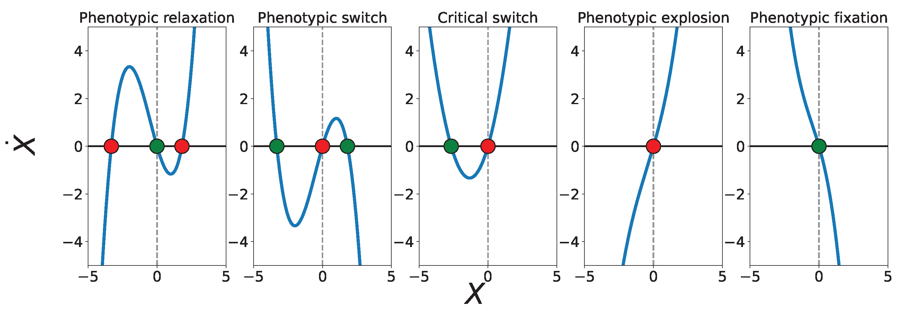
Figure 2.
Phase space diagram of phenotypic space in for positive values where we showed different phases based on and the SNR (). We fix the parameters , and .
Figure 2.
Phase space diagram of phenotypic space in for positive values where we showed different phases based on and the SNR (). We fix the parameters , and .
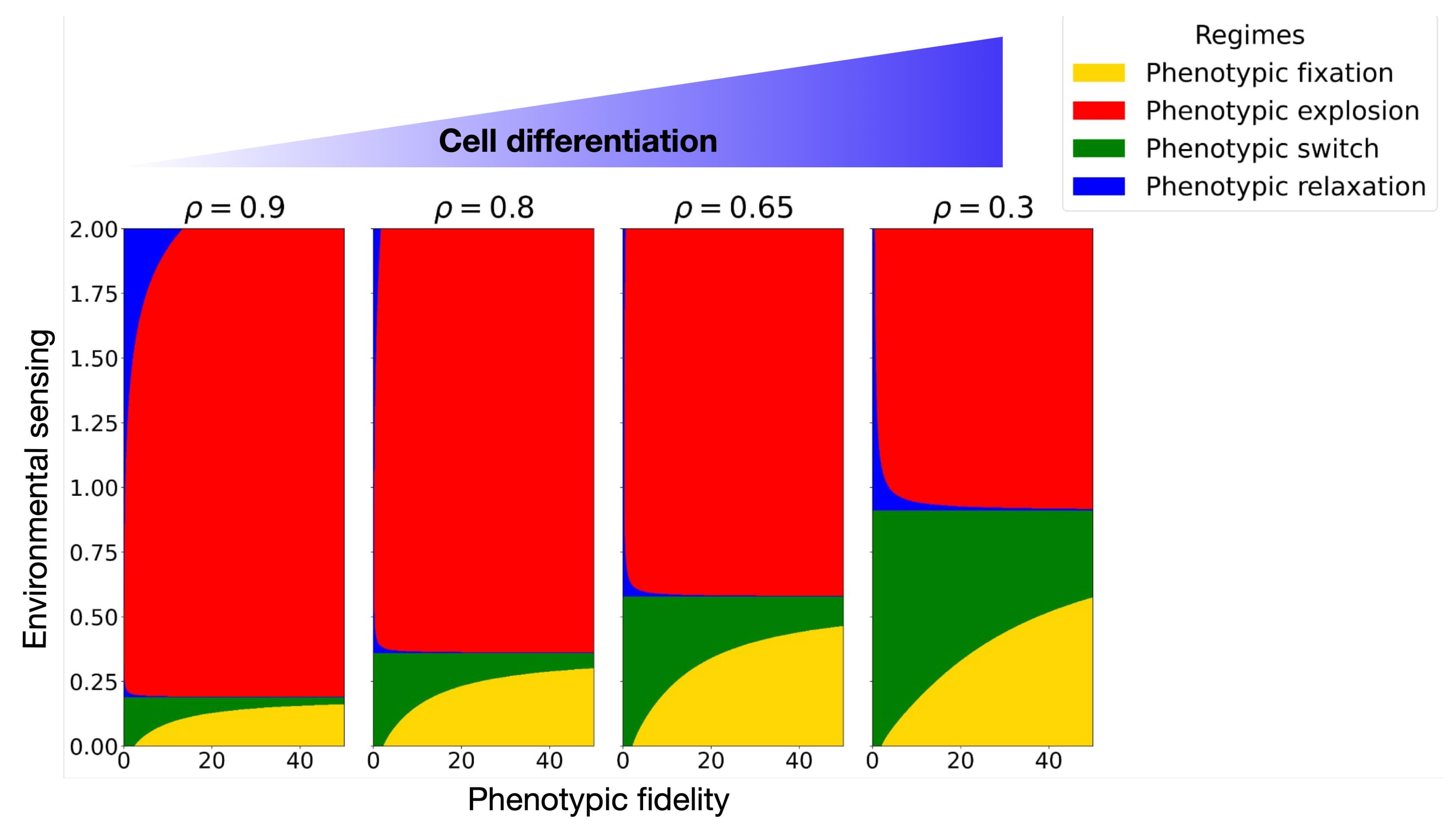
Figure 3.
Plot of the normalized potential function of the phenotype at the limit of and
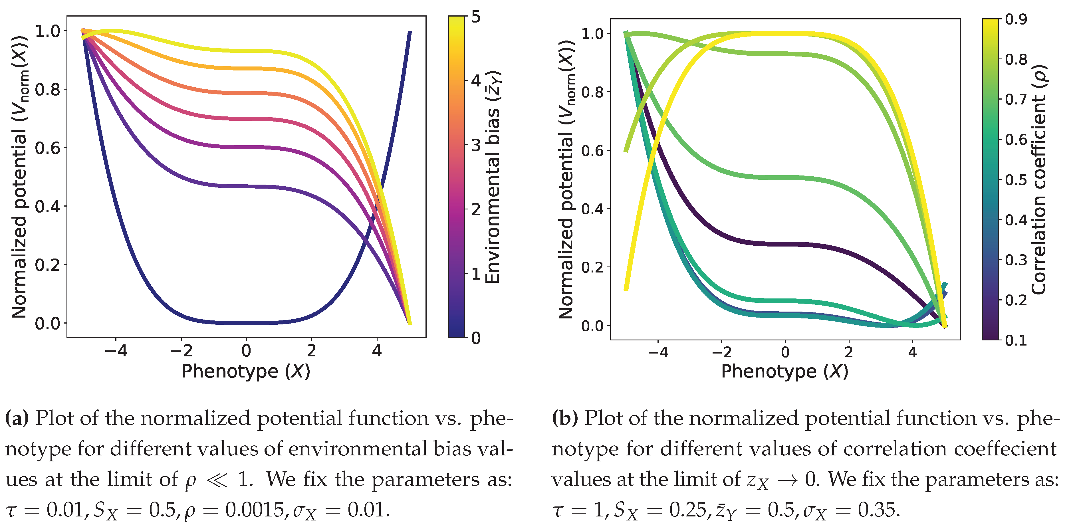
Figure 4.
Carcenogenesis can occur when differentiated cells lose their microenvironmental sensing ability, i.e., increases, entering to the phenotypic explosion regime. The depicted sensing bias vs. SNR phase space has been calculated for correlation coeffecient and for .
Figure 4.
Carcenogenesis can occur when differentiated cells lose their microenvironmental sensing ability, i.e., increases, entering to the phenotypic explosion regime. The depicted sensing bias vs. SNR phase space has been calculated for correlation coeffecient and for .
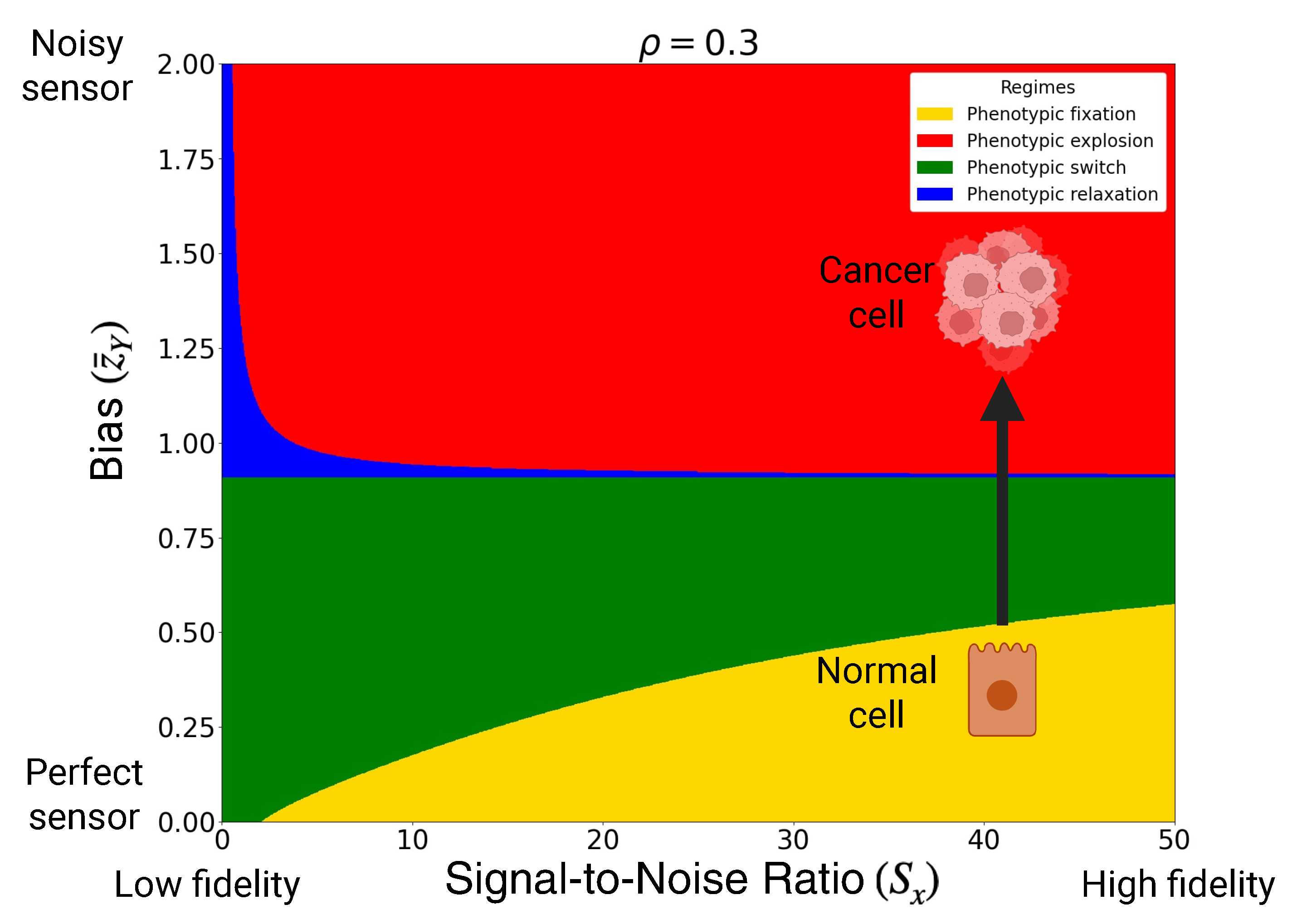
Figure 5.
The plane for different negative intrinsic-extrinsic correlations.
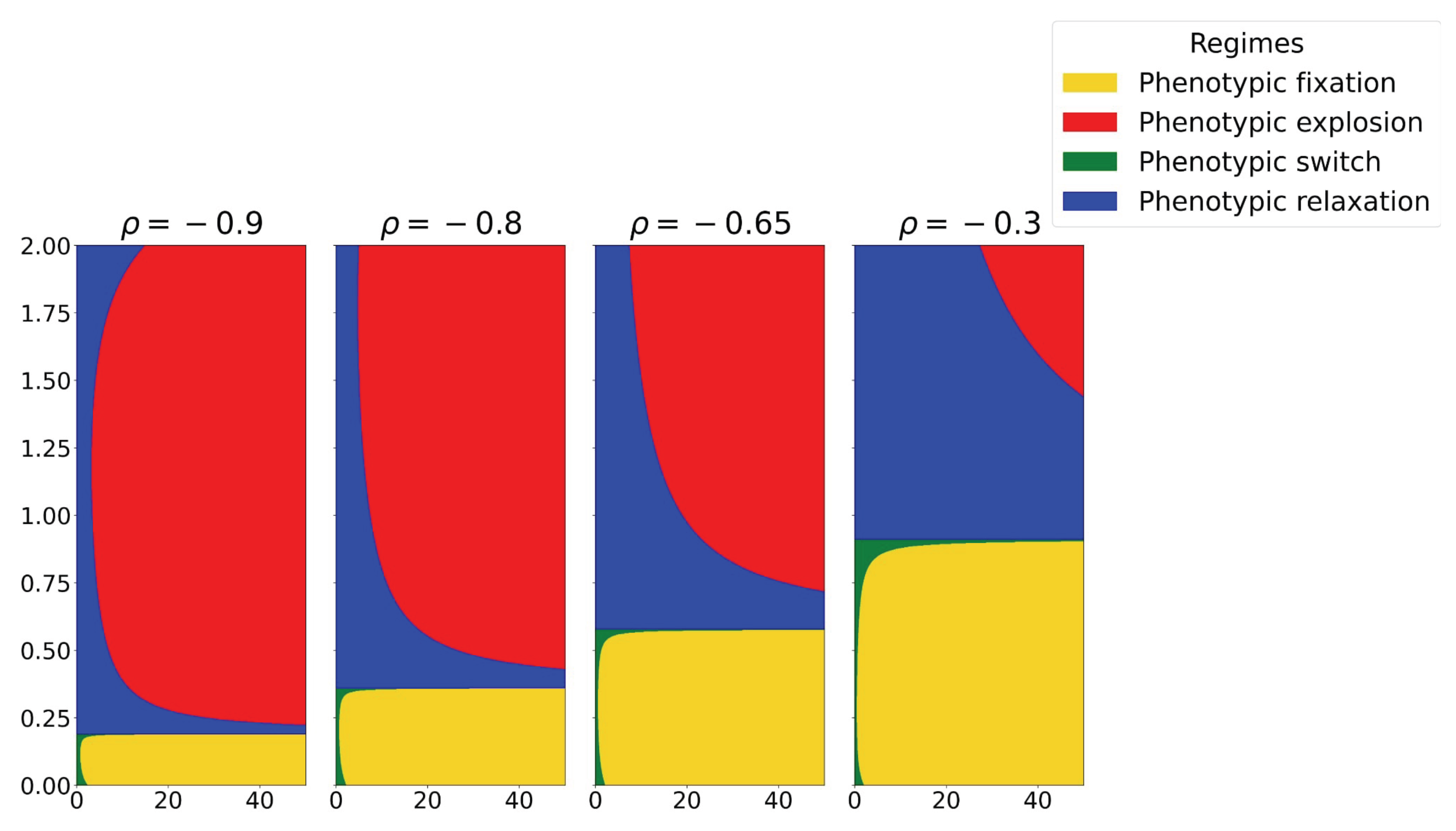
Table 2.
Parameter constellations that define phenotypic regimes and the corresponding potential landscapes.
Table 2.
Parameter constellations that define phenotypic regimes and the corresponding potential landscapes.
| Phenotypic regime | Potential landscape | ||||
| Phenotypic relaxation | any | Two barriers, finite well | |||
| Phenotypic switch | any | Two wells, finite barrier | |||
| Critical switch | any | any | Vanishing barrier | ||
| Phenotypic explosion | Runaway, no minimum | ||||
| Phenotypic fixation | Single deep global well |
Disclaimer/Publisher’s Note: The statements, opinions and data contained in all publications are solely those of the individual author(s) and contributor(s) and not of MDPI and/or the editor(s). MDPI and/or the editor(s) disclaim responsibility for any injury to people or property resulting from any ideas, methods, instructions or products referred to in the content. |
© 2026 by the authors. Licensee MDPI, Basel, Switzerland. This article is an open access article distributed under the terms and conditions of the Creative Commons Attribution (CC BY) license (http://creativecommons.org/licenses/by/4.0/).
Copyright: This open access article is published under a Creative Commons CC BY 4.0 license, which permit the free download, distribution, and reuse, provided that the author and preprint are cited in any reuse.


