
Submitted:
01 January 2026
Posted:
05 January 2026
You are already at the latest version
Abstract
The integration of outdoor camera images with three-dimensional (3D) geographic information on the observed scene has an interest in many applications of video acquisition. To solve this data fusion problem, camera images have to be matched with the 3D geometry provided by the geographic information system (GIS). This paper proposes to use, for a camera of known geographical position, a dense local azimuth-elevation map (LAEM) derived from a gridded digital elevation model (DEM) as data representation to ease the matching operation between GIS data and the image. Such a map assigns to each regularly sampled azimuth and elevation angles pair the geographic point derived from the DEM viewed in this direction. The problem of computing the LAEM from the DEM is closed to the problem of surface rendering, for which solutions exist in computer graphics. However, rendering software cannot be used directly, since their view directions are constrained by the pin-hole camera model and apparent colour rather than position of the viewed point is assigned to the viewing direction. This paper therefore also proposes a specific algorithm for the computation of the LAEM from the DEM. A MATLAB implementation of the algorithm is also provided, which is tailored to process the DEM data set swissALTI3D from the Swiss Federal Office of Topography swisstopo.
Keywords:
gridded DEM
; DEM rendering
; image georeferencing
; geometric camera calibration
; ray casting
1. Introduction
We consider a situation where a pan-tilt-zoom (PTZ) camera fixed in position is used to monitor a landscape. In such a monitoring case, there is often an interest for associating to each camera pixel the geodetic coordinates (e.g. WGS84) [1,2] of the observed physical point. Performing this association is the georegistration of the image or the georeferencing [3] of the image pixels. With the geodetic coordinates of an observed point come along a plethora of possibly interesting geographical informations delivered by a Geographical Information System (GIS) [4].
Digital Elevation Models (DEM) provide information on the three-dimensional shape of the Earth’s surface in the form of elevation values (vertical datum) on a GIS raster (horizontal datum) [5]. Several governmental mapping agencies provide this type of topographical data. The Swiss Federal Office of Topography swisstopo e.g. provides the swissALTI3D [6] raster DEM. DEM are even available at the continent level for Europe as the EuroDEM dataset [7].
Regarding geometry, a camera performs a transformation from the 3D geometric space representing the physical world to the 2D space representing the image. This transformation has been widely studied in the fields of photogrammetry [8], computer vision [9,10], and computer graphics [11]. In most cases of modelling a real camera, this transformation is, in first approximation, a true perspective projection [9]. This is the often called pinhole camera model, referring to an ideal camera where all light rays pass through a pinhole. The transformation can be seen as being composed of three concatenated geometric transformations [9]. The coordinates of the source point in a 3D Cartesian world coordinate system are first transformed into its coordinates in a similar but camera-centric coordinate system, having the Z-axis aligned with the optical axis of the camera. This transformation depends on the camera extrinsic parameters: its pose, made of its position and its orientation. Then, occurs the projection to the image plane, which is perpendicular to the optical axis, giving rise to dimensionless 2D coordinates. Finally, these last coordinates are transformed into pixel coordinates by a 2D transformation depending on the camera intrinsic parameters: focal length, pixel size(s), and origin of the sensor coordinate system.
Except for wide-angle cameras [12], real cameras can be modelled with only a minor modification of the pinhole model [9]: a supplementary transformation is introduced between the second and third transformations mentioned above, in order to take into account the lens distortions. It consists in transforming the dimensionless coordinates resulting from the projection into distorted coordinates by adding a distortion term. It is common from at least the 1980’s [13] to decompose the distortions into a radial component (pure radial displacement) and a tangential component. One reason is that the radial component is often more important than the tangential one and this last one can be therefore often neglected. Furthermore, radial and tangential displacements, increasing with the distance from the image centre, are modelled by polynomial functions of the normalised coordinates.
Let us now assume that the model parameters of a camera monitoring a landscape are known and a DEM of this landscape is available. Then, georeferencing the image pixels is similar to rendering the surface spanned by the DEM with the camera from which we have the model. Indeed, in both cases a point or a small patch of the observed surface is assigned to each pixel. In the case of surface rendering, a colour is then attributed to the pixel according to the light emitted or re-emitted by the surface patch, while, in the case of georeferencing, the geodetic coordinates of the observed surface point or patch are attributed to the image pixel. Solutions for the rendering exist, in particular [14], and can be adapted for georeferencing.
Hence, in the case where a DEM of the landscape monitored by the camera is available, georeferencing the image pixels mainly boils down to finding the parameters of the camera model. This problem, known as geometric camera calibration, has been widely studied in the fields of photogrammetry [15,16] as well as computer vision [9,17,18] and a large number of methods have emerged in both communities. All have in common that the model parameters are estimated from a set of geometric primitives in the physical world and their corresponding geometric entities in the image. In probably the majority of the methods, the world geometric entities are points at the surface of physical objects and their corresponding entities are image pixels or, for more precision, points with sub-pixel coordinates. Prior to the computation of the parameter estimates itself, the first problem to be solved is the selection of calibration points, i.e. points in the scene and points in the image which correspond to each other.
There are two main approaches to solve the problem mentioned hereinbefore. The first one consists in introducing in the scene individual marks or patterns to materialise points, the corresponding points to which are easily detected in the image. Individual marks can be disks with a binary code allowing to identify each of them [19,20], or spheres [21,22]. A rigid planar chequerboard of known square size is used in the well known calibration method developed by Zhang [9,23,24], and implemented in the computer vision library OpenCV [25] as well as in the MATLAB® Computer Vision Toolbox [26]. In this case, the selected points are the corners common to four of the squares.
The second approach is used in camera self-calibration [9,10,27,28,29], which involves multiple slightly different views of the same scene with the same camera. Points of interest are selected in the images and their correspondence from one image to the other is established based on the fact that they match, i.e. their neighbourhoods are similar. With the image points from the different views which correspond to each other, a virtual 3D point is constructed. It is the model of the physical point from which the image points originate. The correspondence of the image points with this virtual 3D point is in this way established automatically.
In the case we are interested in, i.e. a camera monitoring a landscape from which a DEM is at hand, none of the correspondence establishing methods mentioned above can be applied. For the first method, one cannot even imagine modifying the landscape, and accordingly the DEM, with marks detectable in the camera images. On the other hand, if it is easy with a PTZ camera, to generate multiple views of the same landscape, the generated virtual 3D points, mentioned above, will be referenced in a proper coordinate system and will therefore not be directly localisable in the DEM.
Selecting automatically calibration points in the image-DEM pair is the specific problem, this paper is concerned with. Moreover, the physical context is a camera having an oblique view on a landscape, i.e. far from an almost vertical top-down view. This article however does not go so far as to provide a complete solution to the problem. It proposes and describes a particular representation of the DEM, called local azimuth-elevation map (LAEM), the purpose of which is to ease the automatic selection of calibration points. A part from this interest, the LAEM could even be used in a second time for the image georegistration itself, in place of rendering the DEM with the camera model.
Section 2 is dedicated to related work. Then, in Section 3, the LAEM is presented as a particular 3D to 2D mapping. In the same section, a general method is described to compute an LAEM from a DEM in geodetic coordinates. Section 4 is concerned with implementation and experimental results. The implementation adapts the general method to the specificities of the swissALTI3D [6] DEM. Finally, Section 5 summarises the advantages of the particular DEM representation made by the LAEM and gives cues on how correspondences between an image and the LAEM could be found.
2. Related Work
To the best of my knowledge, the problem of selecting automatically points in the camera image and points in the DEM which correspond to each other, has been rarely addressed. However, since the motivation of this focused paper is image georegistration of oblique views, this section will present the related work in this broader view, with emphasis on the determination of the camera pose in a geographical coordinate system. Note that the latter is sometimes referred as the geolocalisation of the image, although the geolocalisation is often understood as concerning only the camera position without its orientation [30]. In the following, unless otherwise specified, geolocalisation will mean both position and orientation of the camera. The related work is organised according to the data used as reference for the georegistration, respectively the geolocalisation:
- orthophoto or georeferenced aerial images,
- georeferenced 3D point cloud,
- digital elevation model (DEM).
Instead of covering numerous publications, the overview gives priority to deep presentation of some examples in each category. Occasionally, personal comments are added.
Geo-Registration/Localisation with Orthophotos or Georeferenced Aerial Images.
Selecting corresponding points in the camera image and in an orthographic satellite image for calibrating the camera is performed semi-automatically in the software developed by Rameau et al. [31]. However, there are two limiting assumptions: the camera must have a rather top-down view on the scene and the calibration points have to lie in a more or less planar surface of the scene. The selection is semi-automatic, since the software user has first to rotate the satellite image until this one is almost aligned with the camera image. Then, a region of interest (ROI) has to be drawn, where the calibration points will be selected automatically.
Shan et al. [32] propose a solution for the georegistration of ground images with the help of georeferenced aerial images. They assume that the ground images have a GPS tag and hence an approximate geoposition. The method they propose is for improving the precision of the geolocation, adding also orientation to the position. Since, there are several ground images of the same scene, a self-calibration of the camera is made and, at the same time, a 3D model of the scene. With the self-calibration, the camera intrinsic parameters are known, but not its pose in a geographic coordinate system. The aerial views are not exactly vertical as is an orthophoto, but the difference between the angle of views of both type of images (terrestrial and aerial) is sufficiently large to make a direct matching between images unsuccessful. With the ground image, the 3D model, and the approximate geolocation of the ground image, they build a synthetic image from the aerial point of view. Then, by matching points between the synthetic image and the aerial image they determine the camera pose in the geographical coordinates system and hence the wanted more precise geolocalisation of the ground image. Comment. Shan et al. have shown impressive results with ground images of landmarks in Rome and aerial images of the city. These are images of man made shapes having a rather simple geometry. The method could be less successful with natural or rural landscapes.
Geo-Registration/Localisation with Georeferenced 3D Point Clouds.
Li et al. [33] propose a method for the geolocalisation of images with the help of georeferenced 3D point clouds. This is an extension to geolocalisation of previous work [34] or similar work by Sattler et al. [35], where the localisation was in a restricted area, typically a town. Let’s start with the localisation in a restricted area. What is called 3D point is in fact not a pure geometric primitive represented by coordinates in a 3D coordinate system, but features also descriptors taken from the images used to construct the geometric point. Hence, for establishing the correspondence between pixels in the image to be localised and some 3D points of the cloud, they use basically the same methods as for matching pixels between images. However, in creating constraints, the existing geometric information, helps for selecting the right corresponding 3D points in the vastness of the cloud. With the corresponding image pixels on one side and 3D points on the other side, the image can be localised by a camera calibration method. In the more recent work [33], the 3D point cloud has a worldwide extension, gathering 3D points from many places (cities) all around the world. A first difference with respect to the previous work is the significant larger size of the cloud, which makes the search of corresponding 2D-3D point pairs more difficult and necessitates a more performant solution. Another difference is that the localisation has to be done with respect to a global coordinate system, i.e. the image geolocalisation is now requested. They perform the georeferencing of the 3D points in using the geotag (latitude and longitude) of the images with which the 3D point has been constructed. As in the case of the localisation in a restricted area, the whole camera pose (3D position and orientation) is determined, but the geolocalisation seems to concern only the horizontal coordinates of the position, since they use precisely geotagged photos to test the precision of their geolocalisation.
DEM- Based Geo-Registration/Localisation.
Härer et al. [36] as well as Milosavljević et al. [37] propose solutions for georeferencing images with a DEM. However, for the step of selecting calibration points, they do it with the help of an orthophoto accompanying the DEM. Moreover, the selection is performed by a human operator. Comment. The manual selection of calibration points is time consuming and can even be difficult, in particular with natural landscapes. For example, ridge summits and passes selected in a camera image can be difficult to identify and localise precisely on an orthophoto or even on a topographical map. Proceeding in the opposite way, singular points detected in the orthophoto can be difficult to identify and localise in the camera image. This occurs when and why the view of the camera on the landscape is oblique, i.e. quite a part from the exactly vertical view of an orthophoto.
Portenier et al. [38] propose a solution for the georegistration of camera images with a DEM for the purposes of measuring snow cover. The camera position is assumed to be known a priori with sufficient precision, its orientation however not. Since they use a simple camera model, without lens distortions and with the optical image centre being in the middle of the digital image, only four parameters have to be estimated for calibrating the camera. Three are extrinsic: the orientation components, and one is intrinsic: the field of view (FOV), which is equivalent to the focal length presented in the introduction. The calibration process is automatic except for the first step, which consists in selecting at least one image with good sky-ground contrast, called the master image. In this image, the visible horizon is then detected and the polyline representing the horizon taken as reference. Then, the space of parameters is discretised within potential ranges of values. Next, for each discrete value of the parameter vector, the DEM is rendered with the camera model having these parameters, the visible horizon is detected and compared with the reference. Finally, the parameters selected for modelling the camera are those minimising the difference with the reference horizon. Portenier et al. noticed that the calibration could not be performed once and for all. Changes in weather conditions and/or human interactions, intentional or not, induce from time to time small changes in camera orientation, requiring a model update. Because it is a cumbersome process, the model is not updated by performing again the calibration. A matching is performed between an image of the moved camera and the master image. The camera rotation and hence the new orientation is then inferred from the pairs of corresponding image points.
Final Comments
The main difficulty in the geolocalisation with orthophotos and georeferenced aerial images is that the image to be geolocalised can differ significantly from the reference image(s). This is not only due to the difference of views, but also to the difference of capture times. In the time interval between the two captures (reference image and image to be geolocalised), drastic changes may have occurred in the scene (e.g. land coverage) or in its illumination (e.g. day/night). Because of these drastic changes, the images can be so different that the geolocalisation becomes impossible.
Geolocalisation with georeferenced 3D point clouds starts in fact with a large dataset of georeferenced photos taken by individuals, from which a georeferenced 3D point cloud is first generated. The 3D points serve to determine the camera pose of the image being geolocalised, but the correspondence between image pixels and some of the 3D points relies on the similitude of this image with the images that have been used to build the 3D points. Hence, the geolocalisation with georeferenced 3D point clouds is subject to the same problem of difference in capture time between images as mentioned before. However in this case, the problem can be mitigated in having at hand many images of the same scene, taken under different lighting and weather conditions. The fact that the 3D point clouds stem from photos taken by individuals during their leisure time has the effect of restricting the use of this geolocalisation method to places which are popular and very much visited, e.g. landmarks in cities.
DEM- based geolocalisation can be associated to geolocalisation with georeferenced 3D point clouds, since a DEM is indeed a georeferenced 3D point cloud. However, the physical reality modelled by the point cloud differs. As seen in the previous paragraph, in the approach named “with 3D point clouds”, the 3D geometry is the one of very much visited built spaces, like landmarks in cities. DEMs in contrary are modelling the ground or, scientifically speaking [5], the interface between the atmosphere and the lithosphere, of large regions. The approaches are therefore not at all rivals but complementaries.
Another difference between both approaches is that DEMs are not built with images from multiple views and therefore do not hold image information which can be used to find the correspondences between the image to be geolocalised and the DEM. It is true that there often exists an orthophoto which can be associated point by point with the DEM. However, because of the problematic large difference in views mentioned in the paragraph dedicated to the geolocalisation with orthophotos, the similarity between the orthophoto and the image to be geolocalised is poor. The operator selecting the calibration points in Milosavljević et al. [37] undoubtedly uses his understanding of the image to be geolocalised and of the orthophoto to make the selection. New paths have to be open for an automatic selection of corresponding points between the image to be geolocalised/georegistered and a DEM. Such an attempt has been made by Portenier et al. [38]. This paper proposes a new one.
3. Local Azimuth-Elevation Map at Camera Position
3.1. Scenario
As explained in the introduction, we consider the case of a PTZ camera fix in position with an oblique view on a natural landscape from which we have a DEM. The typical camera set-up, which is the one used for the experiments (Section 4), is represented in Figure 11. The camera pan axis is more or less vertical and the pan rotation allows a 360° view around the camera position. The proposed method is not exclusive to PTZ cameras. But it is more useful in such a case, where the camera has changing orientation and changing field of view, and it is especially well suited for the camera set-up shown in Figure 1.
Since the camera has a fix position, determining its geodetic coordinates is a one-time procedure, which can be performed at the camera installation or even prior to it. It is is an easy task, especially if the observed landscape is relatively distant from the camera, since in this case, the required positioning accuracy is low. The camera geodetic coordinates can be determined e.g. in using a hand-held global positioning system (GPS). They can also be read on a digital map e.g. on Google Maps [40].
Knowing a priori the camera position and assuming that the DEM is available in the same geodetic coordinate system as the camera position , we will see hereafter that we can represent the DEM in a local coordinate system, where the origin is at the camera position.
3.2. The ENU and AER Local Coordinate Systems
You can refer to Figure 2 for a graphical support to the following text.
Let us consider a point , the camera position in our case, with geodetic coordinates [1,2,41]: geodetic latitude , longitude , and geodetic or ellipsoidal height . Let be the orthogonal projection of on the ellipsoid modelling the Earth. is hence the Euclidian norm of the vector . Let be the plane tangential to the Earth ellipsoid at and be the plane parallel to and containing .
The local East-North-Up (ENU)[1,41] or Local Geodetic Horizon (LZH) [2] coordinate system with origin is a Cartesian coordinate system having the three following to each other orthogonal axis:
- Up is the direction of the vector , denoted by in Figure 2.
- North is the direction at of the meridian, i.e. the ellipse through the geodetic North. It is taken positive towards the geodetic North . In Figure 2, it is represented in the plane parallel to , and denoted by .
- East is the direction orthogonal to the two other ones and so that ENU is a right-handed system. It is denoted by in Figure 2.
Since ENU is a Cartesian coordinate system, it can be used to represent 3D points for camera calibration.
The formulas to transform the coordinates of a point in the geodetic coordinate system to its coordinates in the local ENU coordinate system use an intermediate representation in the Earth-centred, Earth-fixed (ECEF) coordinate system. They can be found e.g. in [1,2]. They are implemented in the MATLAB® Mapping Toolbox by the function geodetic2enu [42] and in the the PyMap3D Python module by the function pymap3d.enu.geodetic2enu [43].
The coordinate transformation is invertible, although there is no explicit form for the geodetic coordinates in function of the ECEF coordinates [1]. The transformation from the ENU coordinates into the geodetic coordinates is implemented in the MATLAB® Mapping Toolbox by the function enu2geodetic [44] and in the the PyMap3D Python module by the function pymap3d.enu.enu2geodetic [45].
The Azimuth-Elevation-Range (AER) coordinate system is the spherical companion of the ENU system [41]. Azimuth and elevation angles are a widely used coordinate system in astronomy to represent the direction from an observer position [46]. The elevation angle is also called sometimes altitude angle. There exist also some variations in the way these angles are measured. In the AER coordinate system, the coordinates of a point P also include the range (or slant range) i.e. the distance from to P. In the following, we use for the AER coordinate system the same conventions as in [41]. Let be the orthogonal projection of the point P on the plane , then:
- the azimuth is the clockwise angle from the axis to the direction ;
- the elevation (or altitude) is the angle between the plane and the direction , positive up, negative down;
- (slant) range r is the Euclidean distance between the points and P.
As in [41], the angles will be expressed hereafter in degrees, in the range for the azimuth and in the range for the elevation .
The formulas for computing the AER coordinates from the ENU coordinates are:
Note that the azimuth is undefined when both and are null. The elevation is undefined when all three ENU coordinates are null, i.e. for the coordinate system origin .
The function geodetic2aer [47] from the MATLAB® Mapping Toolbox and the function pymap3d.aer.geodetic2aer [48] from the PyMap3D Python module allow to perform directly the whole transformation from the geodetic coordinates to the AER coordinates.
The formulas for computing the ENU coordinates from the AER coordinates are:
3.3. Local Azimuth-Elevation Map (LAEM)
3.3.1. Mapping to the Azimuth-Elevation Space
The local azimuth-elevation map (LAEM) is defined as the result of a mapping from the 3D geometric space to the 2D space where the azimuth angle and the elevation angle of a source point are represented in a Cartesian coordinate system. Figure 3 represents this mapping graphically for a point . Since the azimuth is undefined if both and are null, the points belonging to the -axis do not have an image. Furthermore, the image of is a limited domain of . With the conventions adopted in Section 3.2 for the azimuth and elevation angles, the image domain is given by the following ranges on and values: . Note that the domain does not include the elevation values and , because they correspond to undefined azimuth values (points on the -axis).
Even if it is due to a well known property of the inverse trigonometric functions, let us point out the following feature of the image domain. Two points close to each other in the 3D space, one with a positive value and one with a negative value, have distant images. The first image point has a value slightly larger than , while the second one has a value slightly smaller than .
The hereinbefore introduced mapping is similar to the perspective projection realised by a camera of position , in the sense that all points of a half-line from are mapped to a single point. However, there are at least two differences:
- the formula to derive the image coordinates from the AER coordinates of the 3D point is different from the one for deriving the normalised camera image coordinates from the camera centric Cartesian coordinates ,
- a line segment, the endpoints of which map to different points, does not map into a line segment.
3.3.2. LAEM of a Surface
The LAEM of a surface in the 3D space is the mapping of the points belonging to the surface, however with an exclusion condition: from the points belonging to the same half-line from , only the nearest from , i.e. the "visible" one, is mapped. With this condition, the mapping becomes injective. As a consequence, for each pair of values there exists maximum one surface point mapped to this image point. In Figure 4, the points and have the same azimuth and elevation values. However, only the point with smaller range value is mapped to the image point . As a consequence, the unique surface point can be associated to the values and .
3.3.3. Discrete LAEM
For the purpose explained in the introduction, the LAEM has to be discrete, i.e. be a countable set of values. Moreover, the set has to be finite. Among the various possibilities of discretising the LAEM, let us propose this one. The choice is, at least partly, driven by the goal of representing a discrete LAEM as a digital image for an easy storage and processing.
We use a constant sampling interval in azimuth as well as a constant sampling interval in elevation. For convenience, we require that , respectively , divides , formally:
In practice (see Section 4), this constraint is not restrictive, since we use and values as small as .
As it is usual to index the rows of a digital image with i, starting at the top, and the columns with j, starting at left, we index the discrete azimuth values with j, starting with the smallest, and the discrete elevation values with j, starting with the largest. This is represented in Figure 5, where x and y, the commonly used image coordinates [51,52], are also represented. Most of the programming languages start table indexes with 0, this is the assumption for i and j. MATLAB® in contrary starts table indexes with 1. We use the identifiers and for this case. The relationships between both types of indexes are of course simply given by:
In the envisioned camera to landscape configurations, only a limited portion of the elevation range is significant. Let and be the minimal, respectively the maximal, elevation value of interest. For convenience, we require and be both integer multiples of , formally:
With these conditions, the number of discrete elevation values is
and the discrete elevation values are given by the equation
Concerning the azimuth, there may be cases where the full range of values is of interest. However, there also may be cases where the interest is only for a segment of the possible range. It will of course occur that this segment of interest will be on both sides of the azimuth . In the case where the full range of azimuth values is of interest, one could decide to handle easily the angle wrapping, i.e. the transition from to , in expanding the LAEM with an overlap corresponding to the horizontal field of view of the camera. In order to handle all these cases in a simple way, we propose to use unwrapped angle values, i.e. angles values always increasing. Let denotes the unwrapped azimuth and and the minimal, respectively, the maximal, unwrapped angle value. For the full range with overlap mentioned above, one would set for example and , where is the horizontal field of view of the camera . For convenience, we require and be both integer multiples of , formally:
With these conditions, the number of discrete unwrapped azimuth values is:
and the discrete unwrapped azimuth values are given by the equation
The discrete wrapped azimuth angle corresponding to is then simply given by
where the mod function is defined by
3.4. Computing a Discrete LAEM of a Gridded DEM
3.4.1. Methods from Surface Rendering
Section 3.3.1 and Section 3.3.2 show up that computing a discrete LAEM of a surface in 3D space is close to rendering this surface with a camera model, a basic operation in computer graphics [11], and a DEM is basically a surface. It is therefore worth considering if methods used for surface rendering could be adapted to the computation of a discrete LAEM.
Surface rendering starts by establishing the correspondence between image points, i.e. pixels, and points belonging to the surface. For determining this correspondence, there are basically two opposite approaches. The first one proceeds from the scene to the image. The surface is modelled by polygonal patches, either as an exact model or as an approximation obtained by tessellation. Then, the image of the polygon vertices is computed by the true perspective projection modelling the camera. Finally, since linear segments are imaged into linear segments, the polygon edges are drawn as well as the polygon interior areas. This approach is less precise than the second one, because the correspondence is not established individually for each pixel within a patch. However, it is less computation intensive. It is therefore preferred, when the computation time is critical. Whatever the advantages of this approach, it cannot be adapted to LAEM computation, since in this case, as mentioned in Section 3.3.1, line segments are not mapped into line segments.
The second approach proceeds from the image to the scene. This method is known as ray casting since [53]. A ray is traced from the camera centre through each image pixel and the corresponding surface point is determined as the intersection of the ray with the surface. In the case of an LAEM, points of the 3D space of constant elevation and azimuth build also rays from a fixed point, here the coordinate system origin. The only difference with respect to ray casting lies in the distribution of rays in the space. In the case of surface rendering, rays are regularly spaced according to the angle tangent, while in the case of LAEM, they are regularly spaced with respect to the angle value itself. The ray casting method can therefore be easily adapted to LAEM computation. In this paper, we are merely mentioning this possibility, emphasising the method presented in the next section.
3.4.2. Proposed Method: Principle
The method, this paper promotes for computing a discrete LAEM, is different from the surface rendering methods discussed in the previous section. It proceeds mainly from the scene (DEM) to the image (LAEM), but also partly from the LAEM to the DEM. Moreover, it is not linked to rendering the surface represented by the DEM, since it alternatively makes use of the volume of which the DEM is the upper boundary.
Let be a particular element of the DEM with position indices m and n and let us take one of the 4-neighbourhood elements, e.g. . The elementary surface patch used for the LAEM computation is a delimited cross-section of the volume associated with the DEM, as represented in Figure 6. The delimiting edges are: the line segment , the two segments of vertical lines from , respectively , until the minimal elevation value is reached, and the line segment joining these two last points.
The motivation for taking vertical lines is that a DEM provides elevation values (vertical datum) on a GIS raster (horizontal datum) [5]. At the origin of the local ENU coordinate system, the DEM vertical direction is the one of the Up-axis. However, the further a DEM point is from the ENU origin, the larger is the deviation of the vertical direction at that point from the Up-axis of the ENU coordinate system. For a DEM where the elevation is the geodetic height, as we have assumed, the vertical direction is the one of the normal to the underlying ellipsoid. Determining the exact vertical direction at any point of a DEM is however cumbersome and there is generally no need to be very precise on the vertical direction. To have a reference value for the needed precision, let us take a DEM grid resolution of 2 meters, like the DEM used in the experimentation, and the greatest purely vertical drop on the Earth [54], which is 1200 m. The angle formed with respect to the vertical by two consecutive DEM points, one at the top and one at the bottom of the drop, is , equal to . This, rounded to , is the sufficient precision in determining the vertical direction. Given this tolerance, we propose to determine the vertical direction with one among the two following degrees of approximation of the DEM horizontal datum: planar and spheric (see Section 3.4.3).
As explained in the introductory paragraph of the section, the method also involves a procedure from the LAEM to the DEM. It is the following. Let and be the discrete azimuth values corresponding to , respectively , as represented in Figure 6. If the indices and are apart from more than one, i.e. formally: , then for any in-between value j, i.e. , a point is determined on the line segment as the intersection of the plane defined by all the points of same azimuth and the line passing through the points and (see Figure 7).
The ENU coordinates of the point can be easily computed from and the ENU coordinates of and by solving a system of linear equations. Let be the coordinates of in the ENU coordinate system and be those of . Then, the coordinates of in the ENU coordinate system can be found by solving the system of equations:
(13a) is the equation of the plane determined by , while equations (13b) to (13d) are the parametric equations of the line through the points and . Equation (13a) can be replaced by the following explicit equation for :
Once the point has been determined, the patch is "filled" in following down the vertical direction from this point.
3.4.3. Computing DEM vertical lines
As explained in Section 3.4.2, for computing vertical lines from a DEM point, we propose to use approximations of the DEM horizontal datum. We consider two possible approximations: planar and spheric.
Planar Horizontal Datum
If the DEM horizontal datum is the local horizontal plane, as represented in Figure 3, the DEM vertical direction is the normal to this plane. Hence, all points on a vertical line passing through a DEM point have the same coordinates and as this point, as well as the same azimuth and horizontal distance .
Spheric horizontal datum.
At , the origin of the local coordinate system, the curvature of the ellipsoid underlying the DEM depends on the direction considered. According to [1], the minimal radius of curvature is in the meridian, i.e. in the -axis direction, while the maximal is in the perpendicular direction, i.e. the one of the -axis. This last curvature is named curvature in the prime vertical. The values of these two extreme local radii of curvature depend on the geodetic latitude of . The formulae for the radius of curvature in the meridian and for the radius of curvature in the prime vertical are:
where a is the length of the ellipsoid major axis, 6378137.0 m for GRS80, and is the ellipsoid eccentricity squared, 0.006694380022901 for GRS80.
As an approximation of the DEM horizontal datum around by a sphere, we propose to use a radius R between the radius of curvature in the meridian (minimal value) and the radius of curvature in the prime vertical (maximal value), of course augmented by the geodetic height of . Since the geometric mean of both curvatures has a simpler formula than the arithmetic mean, we give preference to the first option. The formula for computing R from the geodetic latitude and height is:
Given a DEM point , the vertical line from this point is normal to the sphere and hence crosses the -axis at the sphere centre C. Let us consider a plane containing and parallel to the horizontal plane through . We can draw a rectangle in this plane as represented in Figure 8(a). The lengths of its edges are the coordinates and of . For any point on the vertical line from , we can do the same: take a parallel plane and draw the rectangle. The edge lengths of each rectangle are the coordinates and of the corresponding point on the vertical line. All the rectangles are similar to each other. Consequently, the coordinates and of the points on the vertical line have a constant ratio or , and therefore a constant azimuth, equal to the one one , that is .
Figure 8(a) represents the vertical line from in the plane . Considering the triangle , it is obvious that the angle between the vertical line from and the -axis depends on the elevation angle and the range of according to the following formula:
The elevation and the range of any point on the vertical line from satisfy the same equation, in particular the points corresponding to the discrete elevation values . The implicit equation for and the corresponding range can be rewritten into:
which can be converted into the following explicit equation for :
Maximal Errors in Vertical Direction
We end this section by proposing an estimated upper bound for the errors in vertical direction committed with each of the two horizontal datum approximations presented hereinbefore.
Let us consider a point in the local horizontal plane distant from by d. This is a particular case of Figure 8(b). The vertical line from is for a spheric model or radius R. The equation (17) for determining the angle between the vertical line from and the -axis takes the simpler form: .
In the case of the planar approximation, the vertical direction at given by the model is the one of the -axis. If we assume that the right vertical direction is the one given by the sphere of radius R, the error is measured by the angle . For a given distance d, is maximal for R being minimal. The minimal value for R is the radius of curvature in the meridian at the equator, i.e. . We hence consider as an upper bound of the error in vertical direction made in using the planar approximation.
Around , the ellipsoid modelling the Earth lies between a sphere of radius and a sphere of radius . The angle error in estimating the vertical direction with a sphere of mean radius, as we do with the spheric approximation, should be smaller than the difference between the vertical directions determined by both spheres. This difference is maximal at the equator. We consider therefore as an upper bound of the error in vertical direction made in using the spheric approximation.
Table 1 gives the numerical values of , respectively at different distances d of . The used reference ellipsoid is GRS80. Given the tolerance of for a grid resolution of 2 meters computed in Section 3.4.2, it follows from the numerical values of Table 1 that the planar approximation can be used up to a distance of about 10km and that the spheric approximation has no practical limits for this tolerance.
3.4.4. Detailed Method Description
We use a scalar two-dimensional array to represent the LAEM. Hereafter, we will denote an array element by and the whole array by . In the case of the planar approximation, d is the horizontal distance , while in the case of the spheric approximation, d is the slant range r. In any of these cases, the triplet represents a point of the 3D space, the coordinates of which can be computed in any coordinate system: AER, ENU, geodetic,…
The pseudo-code of listing 1 explains in detail how the LAEM is computed from a gridded DEM, the elements of which are denoted by . We only add information where we estimate necessary, referring to the code by the line number.
| Listing 1. LAEM computation | ||
| 1 | % compute coordinates of DEM points | |
| 2 | for each : | |
| 3 | compute | |
| 4 | % add coordinates of interpolation points | |
| 5 | for each : | |
| 6 | for each and each : | |
| 7 | compute making use of (14a), (13b), (13c), and (13d) | |
| 8 | % fill the LAEM | |
| 9 | ||
| 10 | for each : | |
| 11 | if : | |
| 12 | for each : | |
| 13 | % spheric approximation | %planar approximation |
| 14 | compute with equation (19) | nop |
| 15 | ||
- line 3:
- The values , , and result directly from the representation of in the AER coordinate system. represents either the horizontal distance (planar approximation) or slant range (spheric approximation) of . and determine the position of in the LAEM. They are derived from the azimuth and the elevation of according to the choices that have been made in Section 3.3.3 for the discretisation of the space. The equations are:where is the unwrapped azimuth angle, related to the azimuth angle by:
- line 7:
- The interpolation has been explained in Section 3.4.2 and illustrated in Figure 7. j determines the discrete unwrapped azimuth angle . The explicit equations (14a), (13b), (13c), and (13d) allow to compute from the ENU coordinates of the interpolation point between and , respectively between and . From the ENU coordinates of the interpolation point, the corresponding and values are derived with the ENU to AER coordinate transform. Finally, , determining together with j the position of in the LAEM, is computed from by equation (20b). This new coordinate triplet is added to the set (or list) of coordinates that will be browsed to fill the LAEM.
- lines
- 9 and 11: According to Section 3.3.2, from the points having same LAEM position, we keep only the "visible" one, i.e. the one with smallest d value. The LAEM is hence initialised at line 9 with a specific value, larger than any possible d value, here the choice . Furthermore at line 11, the position of the currently evaluated point is only updated, if the value is smaller than the value stored in at this position.
- lines
- 12 to 15: together with determine the position of the currently evaluated DEM point. The following i values, each together with , determine the LAEM positions of 3D points located on the vertical line down from the DEM point. According to Section 3.4.3, they have the same azimuth and hence the same j value. Moreover, in the case of the planar approximation, they have the same horizontal distance value as the as the DEM point, i.e. . In the case of the spheric approximation, the point slant range is computed from by equation (19). The LAEM is updated with these respective values: and . Note that it is not necessary to test if the d value of the points on the vertical line is smaller than the value existing in the LAEM at that position, because the truth follows directly from the truth of the condition for the DEM point.
3.4.5. DEM Downsampling as Preprocessing
The discrete LAEM as defined in Section 3.3.3 has a constant azimuthal resolution . The corresponding horizontal spatial resolution , as defined in Figure 9, varies with the horizontal range according to the formula:
For an azimuthal resolution of , as used in the experimental part (Section 4), the spatial resolution takes the value 0.1745 m at an horizontal distance of 1 km, 1,745 m at 10 km, and 17.45 m at 100 km. At a distance of about 10 km, the spatial resolution is hence about the same as the 2 meters grid resolution of the used DEMs. Figure 10(a) shows the situation at a distance significantly lower than the balance distance of equal resolutions, while Figure 10(b) shows the situation at a distance significantly higher than the balance distance.
In the situation of Figure 10(a), the interpolation ensures that the LAEM gets a value at all discrete azimuth values, also at those situated between DEM points. In the situation of Figure 10(b), several neighbouring DEM points are mapped to the same j value. The condition of listing 1 line 11 however selects only the nearest one. This performs implicitly a subsampling of the DEM points, but without any prior aggregation of those points into a representation of the group. In digital signal processing [55] and image processing [9], such a subsampling is known as performing the unwanted effect of aliasing and has to be preceded by a low-pass filtering to avoid it. Here, we only advice to perform, where it is needed, a correct downsampling of the DEM as preprocessing. However, so far, we have not worked out a solution where a correct downsampling is integrated in the LAEM computation presented in Section 3.4.4.
4. Implementation and Experimental Results
4.1. The swissALTI3D DEM
swissALTI3D [6] is a raster digital Elevation Model (DEM) available currently in the Swiss LV95 [56] (for grid) and LN02 [57] (for height) coordinate systems. All coordinates are in meters. The data exist at two grid resolutions: 0.5 and 2 meters.
The DEM is freely downloadable from [6]. It is split into files (tiles) corresponding to a terrain square of 1 km by 1 km, available in 2 formats: Cloud Optimized GeoTIFF (COG) and zipped ASCII X,Y,Z. ESRI ASCII GRID is also available on request. The selection of the tiles occurs by clicking on a zoomable map of Switzerland (default). Alternative solutions are rectangle and polygonal selection, as well as selection by political regions: canton or municipality. Download of the whole data set is also an option. For a small number of selected tiles (e.g. square of 6 by 6 tiles), the files can be downloaded individually. For larger selections, only a csv file with the list of the file links, e.g. https://data.geo.admin.ch/ch.swisstopo.swissalti3d/swissalti3d_2019_2594-1119/swissalti3d_2019_2594-1119_2_2056_5728.tif, is directly downloadable from the web page.
4.2. Camera Set-Up and Images
The camera used for the experimentation is an AXIS M5525-E PTZ Dome Network Camera, featuring endless pan, 0-90° tilt, and 10x zoom capabilities. For other camera features, we let the reader refer to the product support web page [60]. The camera has been installed on the roof of the building ENP23 of the HES-SO Valais-Wallis in the town of Sion. This high position gives a view above the neighbouring buildings on the side slopes of the Rhône Valley.
While dome cameras are often installed at a room ceiling to monitor the half-space below the ceiling. In this set-up, the camera has been installed upside down to monitor the half-space above the building roof. To allow a view above surrounding objects on the roof, the camera has been fixed at the top of a 2000 mm high by 800 mm wide frame as shown in Figure 11(a). The frame has been levelled with a spirit level. This mechanical structure has been selected to easily allow, on demand, the installation of other monitoring sensors. As visible in Figure 11(b), a crown-shaped hardware mask has been 3D printed and glued on the camera casing, to avoid collecting privacy sensitive data in taking pictures of the neighbouring buildings.
Figure 12 shows a typical image from the camera. The black area in the bottom of the image is due to the privacy mask. Pictures have been systematically taken with this camera over a whole year at a mean rate of two sessions per day. A subset of the sessions is publicly available from the B2SHARE repository [61] under license “Creative Commons Attribution 4.0 International”. For demanding access to the whole dataset, use the contact information given at [61].
4.3. Determining the Camera Position
As a first step, the camera position has been determined on the online digital map of Switzerland of the Swiss Federal Office swisstopo [62]. Selecting the Aerial imagery as background, it is easy to identify the camera location on the building roof and let the position coordinates being displayed in clicking on the right mouse button. Figure 13 shows the displayed coordinates.
The given elevation value, in the LN02 coordinate system, is of course not the altitude of the camera, but the one of the ground level. To determine the height of the camera position with respect to the ground level, we have used a laser distance meter Leica Disto X4 and found the LN02 altitude of the camera to be 517.5m.
4.4. Preselection and Download of the DEM tiles
We have opted for the COG file format and the 2 meters resolution, since we have estimated this one quite sufficient for modelling the scene monitored by the camera.
Because the part of the Rhône Valley where the camera is located is also a part of the Canton Valais, a simple preselection of the tiles was made by choosing the option “Selection by canton” and then entering the name “Valais”. This generated a csv file to be downloaded. We downloaded the file, which contained, in a single column, a list of 5562 hyperlinks to the individual tile files. The files themselves were downloaded with the help of a MATLAB® m-file reading the csv file, performing an http request for each hyperlink in the list, and saving the received data as a file into a local directory.
Even if it is not significant, we want to mention that the downloaded DEM files do not fully cover the landscape visible from the camera, since a very small portion of the visible terrain is in France and not surveyed by the Swiss Office of Topography. The concerned region is in a very small angle of view and at more than 40 km from the camera.
4.5. LAEM Computation
4.5.1. Computation of the Geodetic Coordinates
As mentioned in Section 4.1, the swissALTI3D DEM uses Swiss specific coordinate systems for both the horizontal and the vertical datum. In Section 4.3, the camera position has been determined in the same coordinate systems. The transformation into the local AER coordinate system described in Section 3.2 being from a geodetic coordinate system, we have, for using it, first to transform the DEM and the camera position into a geodetic coordinate system.
The LN02 elevation values are orthometric heights. Their conversion into geodetic heights cannot be performed by a mathematical formula, because they are of different natures. The first elevation is linked to gravity, while the second one is linked to geometry. The conversion into the geodetic heights necessitates the official Swiss geoid model CHGeo2004 [63]. The Swiss Federal Office of Topography swisstopo provides the free online service REFRAME to perform coordinate transforms, in particular the transformation of the LN02 heights into the geodetic heights on the Bessel 1841 ellipsoid. This is the transformation we need.
Swisstopo offers different possibilities for using the REFRAME service. First, the transformation can be performed via the web page [64], where a file can be uploaded, the transformation selected, and the resulting file downloaded. This is an easy way for transforming one or a few files. It is also possible to perform coordinate transforms via the REST API [65], but one http request has to be done for each pair or triplet of coordinates. Swisstopo also provides software libraries (DLL, JAR) [66] to enable the use of the REFRAME service within software applications. However, the provided functions also perform the coordinate transform for a single point only. The last offered possibility is the use of the GeoSuite software for Windows [67], provided freely by swisstopo. This software allows to perform transforms of multiple files in batch. The module REFRAME and the type of transformation can be easily selected as represented in Figure 14. The only drawback is that is does not accept swissALTI3D files in GeoTIFF format for the needed altitude transform.
For the transformation of the camera altitude from LN02 to geodetic, we used the REFRAME REST API, performing the http request:
http://geodesy.geo.admin.ch/reframe/ln02tobessel
?easting=2594281.5&northing=1119555.5&altitude=517.5
We received back the following data:
{"type": "Point", "coordinates": [2594281.5, 1119555.5, 518.1399090414052]}.
The camera altitude on the Bessel 1841 ellipsoid has been then recorded as 518.14 m.
For the altitude transformation of the swissALTI3D files, we chose the batch ability of the GeoSuite software, combined with a transformation of the swissALTI3D files from GeoTIFF to XYZ, before the altitude transformation, and from XYZ to GeoTIFF after the transformation. We made a test with a batch of 500 files and noticed that the transformation was very resource demanding. Since the difference between the LN02 height and the geodetic height is in the magnitude of not more than 10 meters, we have decided to start the processing with the LN02 heights and perform the transformation only for the tiles that actually remain after the selection described in Section 4.5.2 and Section 4.5.3.
For the transformation of the LV95 coordinates into the geodetic latitude and longitude on the Bessel 1841 ellipsoid, for both the camera position and the DEM files, we simply used the projinv function [68] of the MATLAB® Mapping Toolbox. The projected Coordinate Reference System (CRS) object to be passed to the function as first parameter can simply be retrieved from any swissALTI3D COG file when reading the file with the function readgeoraster [69]. If R is the variable receiving the second output argument of readgeoraster, the value to be passed to projinv is simply R.ProjectedCRS.
4.5.2. Tile-Level Processing
The preselection of the swissALTI3D tiles performed in Section 4.4 is quite broad. Many of the preselected tiles model landscape which is not at all visible from the camera position. To avoid useless processing, a processing of lower computational complexity is performed at the tile level. This processing extracts information with which it will be possible, while filling the LAEM tile by tile, to decide if a new tile has to be processed in the way given by listing 1 or not at all, because it contains no point visible from the camera position.
In Section 4.5.1, we have explained that the transformation of the LN02 heights into geodetic heights by the swisstopo REFRAME service was too much resource demanding to perform it on the whole preselected files. Hence, the processing at tile level is performed with tiles in LN02 heights. If the transform would have been made, the same processing step would have been performed, but with tiles in geodetic heights. We therefore consider both cases.
To avoid confusion between the local ENU and the LV95 coordinate systems, we will use in the following the symbol u for the easting LV95 coordinate (instead of x) and v for the LV95 northing coordinate (instead of y). A swissALTI3D tile is rectangular in the LV95 coordinate system. Let , and , be the extremal easting, respectively northing coordinates. For adjacent tiles in east direction, of the eastern tile is strictly larger than of the western tile. The difference is equal to the DEM resolution (2 meters for our choice). The same holds for the northing coordinate v.
The pseudo-code of listing 2 describes the processing performed at the tile level. We add the necessary complementary information, referring to the code by the line number.
| Listing 2. Tile-level processing | |
| 1 | for each tile : |
| 2 | determine |
| 3 | if , current tile is |
| 4 | for each tile in : |
| 5 | determine |
| 6 | build B according to equation (23) |
| 7 | compute for each |
| 8 | compute with equation (24) |
- line 2:
- are easy to determine. If the tile format is ASCII XYZ, they can be determined directly from the file name. If the tile format is COG, they can also be found in the file metadata.
- line 3:
- If the LV95 coordinates of the camera satisfy this condition, the camera position is within the tile currently considered. This tile is denoted by . As explained hereinbefore, adjacent tiles do not have common extremal coordinates, so that the camera position cannot be in more than one tile. In contrary, it can happen that the camera position is between two adjacent tiles. In this case, is simply the empty set ∅.
- line 5:
- Extremal height values and (either LN02 or geodetic, depending on the file content) can be easily determined by scanning once the file. Performing the processing with original tiles, containing LN02 heights, we increase by a safety margin of e.g. 20 meters, in order to ensure not missing visible points when discarding a tile. Having tiles in geodetic heights, can be kept as it is.
- line 6:
- With the extremal coordinate values , and , we build a tile bounding box, which is a rectangular cuboid in the coordinate systems LV95/height. For the reason that will become clear further, we do not only use the 8 vertices of the rectangular cuboid, but also the edges. The set of coordinates is hence:
- line 7:
- The coordinates of the points belonging to B are transformed into the values , , and d of the local coordinate system, where d is the horizontal distance in the case of the plane approximation of the DEM horizontal datum and d is the slant range r in the case of the spheric approximation. Note that the height is not transformed from LN02 to geodetic. It is kept in the same height coordinate system as the tile.
- line 8:line 8:
-
Following extremal , , and d values are computed for the points belonging to B:We use T for tile in the notation in order to not confuse these and values with the extreme LAEM azimuth and elevation values introduced in Section 3.3.3.Without demonstration, we claim that the values , , and of any tile point P satisfy:Note that the statement is not true, if B is reduced to the 8 vertices of the rectangular cuboid.
4.5.3. LAEM Computation with Tile Sorting and Filtering
In this section, we describe how the LAEM is computed tile by tile, making use of the information extracted from the tiles, to decide if the current tile has to be processed in the way given by listing 1 or not at all, because it does not contain any point visible from the camera position.
The condition for the decision uses from the tiles the four values computed by Equation (6): , , , and , and from the LAEM the apparent horizon, i.e. the coordinates of highest elevation for which the LAEM value is not . The azimuth values and determine an azimuthal sector, which we will denote by . Then, the condition for a tile to be processed is that either the maximal tile elevation is larger than the minimal elevation of the apparent horizon in the sector or the minimal tile distance is smaller than the maximal LAEM value on the apparent horizon in the sector . A formal description of the condition will be provided while commenting the pseudo-code of listing 3.
We keep the information on the apparent horizon in a one-dimensional array , the length of which is equal to the number of LAEM columns, containing the indexes of the highest discrete elevations. The array element of position j, denoted by , is hence formally defined by the following equation:
The minimum function is used instead of the maximum, because of the choice made in Section 3.3.3 of indexing the discrete elevations from the highest (top) to the lowest (bottom).
The pseudo-code of listing 3 describes the LAEM computation tile by tile, checking for each tile if they they have to be processed because they may contain visible data. We add the necessary complementary information, referring to the code by the line number.
| Listing 3. LAEM computation with tile sorting and filtering | |
| 1 | %Initialise and |
| 2 | , |
| 3 | update and with |
| 4 | for each tile in sorted ascending according to : |
| 5 | compute |
| 6 | compute |
| 7 | if : |
| 8 | update and with |
- lines
- 3 and 8: The update of is performed in the way described in listing 1. The update of is simply performed in inserting the following instruction after the line 11 of listing 1: if .
- line 4:
- Doing the processing without sorting the tiles would give the same final LAEM but would necessitate to process more tiles.
- line 5:
- From and , the indexes of the corresponding discrete azimuth values and are computed using the equations (21) and (20a). From , the index of the corresponding discrete elevation value is computed using the equation (20b).
- line 6:
-
These are extremal values in the section going from to of the apparent horizon . is the minimal elevation in the section, formally:is the maximal LAEM value in the section, formally:
- line 7:
- This is the formal expression of the condition expressed with words at section start.
4.6. Results
The MATLAB® implementation and the results date from the project time (Dec. 2021-Sept.2023). Only the planar approximation of the DEM horizontal datum has been implemented. The LN02 to geodetic height transformation with REFRAME was tested, also the JAR library, but performed neither on the whole set of the preselected tiles, nor on the set of the finally selected ones.
Figure 15, dating from Sept. 2023, shows the greyscale coded LAEM obtained from the camera position with an angular resolution of in azimuth , as well as in elevation . The range in azimuth is and the one in elevation is . The north-east (azimuth ) to south-west (azimuth ) orientation of the Rhône Valley can be easily recognised. The highest elevation of the apparent horizon has a value of about and is southwards, at an azimuth of about .
Figure 16 represents in an image the preselected as well as the finally selected tiles. Each tile is represented by a small square. The tile containing the camera position is the isolated white square, close to the image centre. The tiles not containing the camera position, which have been fully processed are in red. There are 805 such tiles. The tiles which have been selected, but finally not processed for filling the LAEM are in black.
5. Discussion
In this paper, I have proposed a new representation of a digital elevation model (DEM) called local azimuth-elevation map (LAEM) and I have described a method to compute this representation. The method has been implemented in MATLAB® and tested on the swissALTI3D DEM published by the Swiss Federal Office of Topography swisstopo. The implementation has required completing the general method with processing specific to the DEM delivered by swisstopo. That is transforming the Swiss specific coordinates into geodetic coordinates and dealing with the tiling of the DEM. Both, the method principle and its implementation, have been described with sufficient details in order to be analysed on correctness and be exactly reproduced by any interested reader.
The LAEM representation and the method for its computation have been developed in a research project having as goal: the calibration of a PTZ camera with the help of DEM data. Notwithstanding the goal, the LAEM features per se the following advantages:
- It contains only and totally the portion of a DEM which is visible from a given position.
- It is not a subset in any order, but DEM points are arranged with a spatial consistency.
- The dimensionality is reduced from 3D to 2D. The LAEM is comparable to an image of the DEM but with the distance information (horizontal distance or slant range r) and another 2D coordinate system.
- The scalar value in the 2D space, the slant range r in the spheric approximation case, is rotation invariant.
Regarding the project goal (camera calibration), where the key problem was to find points in the camera image and points in the DEM which correspond to each other, the new representation is an important step on the way to the problem solution for the following reason: it narrows the set of DEM candidates and arranges them in 2D in a way consistent with the arrangement of their projection in the image . For achieving the goal, I launch the following ideas, opening paths for future research:
- Depth
- map The LAEM is a depth map, it is similar to the output of a LiDAR. Techniques from the fusion of LiDAR and camera data [70] can be used. In particular, one could work on the similarity between discontinuities [71] of the LAEM and image edges [9]. Note that this is a generalisation of the approach used by Portenier et al. [38], who used the similarity of the apparent horizon in the image and the one in a synthetic image generated from the DEM.
- GIS
- augmented LAEM The final goal of the camera calibration is the georeferencing of the camera image to be able to enrich the image with GIS information. Changing the ordering of the procedure, i.e. starting by enriching the LAEM with GIS information, e.g. roads, public lights,…could help in finding correspondences between the camera image and the LAEM. The use of an orthophoto to complement the LAEM, the drawback of which has been discussed in Section 2, would also belong to this approach.
- Self-
- calibration In the case of a PTZ camera, a self-calibration can be performed. With it comes along a 3D point cloud. The camera pose is relative to this 3D point cloud. It is then possible to align the 3D point cloud with the LAEM and, by the way, get the pose of the camera in a geographic coordinate system. For aligning the 3D point cloud generated by the self-calibration with the LAEM, the well-known RANSAC algorithm [9] can be used. Another idea is to transform the 3D point cloud in AER coordinates and use the rotation invariance of the range component r and the LAEM value to preselect points which can correspond to each other.
Last but not least, as mentioned in Section 3.4.5, I propose to integrate a downsampling procedure in the method presented for computing the LAEM.
Funding
This research was conducted from Dec. 2021 to Sept. 2023 when I was with the HES-SO Valais-Wallis, Institute of Systems Engineering. It has been funded by the HES-SO University of Applied Sciences and Arts Western Switzerland and its faculty Engineering and Architecture under the title “Calibration d’une caméra PTZ à l’aide d’un modèle numérique de terrain” and grant number 115161. The paper summary was written at that time. The paper content has been drafted in the late 2025 without external funding.
Data Availability Statement
The original data from the Swiss Federal Office of Topography swisstopo used in the experiments are openly available at https://www.swisstopo.admin.ch/en/height-model-swissalti3d. A set of images taken with the camera set-up described in the experimental part is freely available in the B2SHARE repository at DOI:10.23728/b2share.1474166f2e024413a181089253
Acknowledgments
I would like to thank Ms. Lizzie Lian from MDPI for having sent me an invitation to submit a contribution to this journal. Without this invitation, I would probably not have taken the time of writing this article. I am also grateful to my wife for having given me the time to do it.
Conflicts of Interest
The author declares no conflicts of interest.
Abbreviations
The following abbreviations are used in this manuscript:
| 2D | two-dimensional |
| 3D | three-dimensional |
| AER | azimuth-elevation-range |
| ASCII | American Standard Code for Information Interchange |
| COG | Cloud Optimized GeoTIFF |
| DEM | Digital Elevation Model |
| ECEF | Earth-centred, Earth-fixed |
| ESRI | Environmental Systems Research Institute, Inc. |
| FOV | field of view |
| GIS | Geographic Information System |
| GRS80 | Geodetic Reference System 1980 |
| LGH | Local Geodetic Horizon |
| LGHS | Local Geodetic Horizon System |
| LAEM | Local Azimuth-Elevation Map |
| LN02 | Swiss national levelling network 1902 |
| LV95 | Swiss national survey coordinate system 1995 |
| PTZ | pan-tilt-zoom |
| ROI | region of interest |
References
- Meyer, T. Grid, ground, and globe: Distances in the GPS era. Surveying and Land Information Systems 2002, 62, 179–202. [Google Scholar]
- Van Sickle, J. Basic GIS coordinates, third edition ed.; CRC Press, Taylor & Francis Group: Boca Raton, 2017. [Google Scholar]
- Hastings, J.T.; Hill, L.L. Georeferencing. In Encyclopedia of Database Systems; Liu, L., Özsu, M.T., Eds.; Springer US: Boston, MA, 2009; pp. 1246–1249. [Google Scholar] [CrossRef]
- Shekhar, S.; Xiong, H.; Zhou, X. (Eds.) Encyclopedia of GIS, 2 ed.; Springer Cham, 2017. [Google Scholar] [CrossRef]
- Guth, P.L.; Van Niekerk, A.; Grohmann, C.H.; Muller, J.P.; Hawker, L.; Florinsky, I.V.; Gesch, D.; Reuter, H.I.; Herrera-Cruz, V.; Riazanoff, S.; et al. Digital Elevation Models: Terminology and Definitions. Remote Sensing 2021, 13. [Google Scholar] [CrossRef]
- Federal Office of Topography swisstopo. swissALTI3D. Available online: https://www.swisstopo.admin.ch/en/height-model-swissalti3d (accessed on 2025-11-01).
- EuroGeographics AISBL. Open Maps for Europe | Eurogeographics. Available online: https://www.mapsforeurope.org/datasets/euro-dem (accessed on 2025-10-30).
- McGlone, J.C. (Ed.) Manual of photogrammetry, sixth ed.; American Society for Photogrammetry and Remote Sensing: Bethesda, Md, 2013. [Google Scholar]
- Szeliski, R. Computer Vision: Algorithms and Applications, 2nd ed.; 2022; Available online: https://szeliski.org/Book (accessed on 2025-11-03).
- Hartley, R.; Zisserman, A. Multiple View Geometry in Computer Vision, 2 ed.; Cambridge University Press: Cambridge, 2004. [Google Scholar] [CrossRef]
- Akenine-Möller, T.; Haines, E.; Hoffman, N.; Pesce, A.; Iwanicki, M.; Hillaire, S. Real-Time Rendering 4th Edition; A K Peters/CRC Press: Boca Raton, FL, USA, 2018; p. 1200. [Google Scholar]
- Huai, J.; Shao, Y.; Jozkow, G.; Wang, B.; Chen, D.; He, Y.; Yilmaz, A. Geometric Wide-Angle Camera Calibration: A Review and Comparative Study. 2024. [Google Scholar] [CrossRef] [PubMed]
- Slama, C.C. (Ed.) Manual of photogrammetry, fourth ed.; American Society for Photogrammetry: Falls Church, Va, 1980. [Google Scholar]
- Bösch, J.; Goswami, P.; Pajarola, R. RASTeR: Simple and Efficient Terrain Rendering on the GPU. In Proceedings of the Eurographics 2009 - Areas Papers; Ebert, D., Krüger, J., Eds.; The Eurographics Association, 2009. [Google Scholar] [CrossRef]
- Remondino, F.; Fraser, C. Digital camera calibration methods: considerations and comparisons. In Proceedings of the Proceedings of the ISPRS Commission V Symposium ’Image Engineering and Vision Metrology’; Maas, H.G., Schneider, D., Eds.; International Society for Photogrammetry and Remote Sensing: Dresden, Germany, 2006; pp. 266–272. Available online: https://www.isprs.org/proceedings/xxxvi/part5/paper/remo_616.pdf (accessed on 2025-11-08).
- Hieronymus, J. Comparison of methods for geometric camera calibration. ISPRS-Archives 2012, XXXIX-B5, 595–599. [Google Scholar] [CrossRef]
- Salvi, J.; Armangué, X.; Batlle, J. A comparative review of camera calibrating methods with accuracy evaluation. Pattern Recognition 2002, 35, 1617–1635. [Google Scholar] [CrossRef]
- Long, L.; Dongri, S. Review of camera calibration algorithms. In Proceedings of the Advances in Computer Communication and Computational Sciences; Bhatia, S.K., Tiwari, S., Mishra, K.K., Trivedi, M.C., Eds.; Singapore, 2019; pp. 723–732. [Google Scholar]
- van den Heuvel, F.; Kroo, R. Digital close-range photogrammetry using artificial targets. In Proceedings of the XVIIth ISPRS Congress Technical Commission V: Close-Range Photogrammetry and Machine Vision; Fritz, L.W., Lucas, J.R., Eds.; 1992; Vol. XXIX Part B5, pp. 222–229. Available online: https://www.isprs.org/proceedings/xxix/congress/part5/222_XXIX-part5.pdf (accessed on 2025-11-08).
- Wang, W.; Pang, Y.; Ahmat, Y.; Liu, Y.; Chen, A. A novel cross-circular coded target for photogrammetry. Optik 2021, 244, 167517. [Google Scholar] [CrossRef]
- Luhmann, T. Eccentricity in images of circular and spherical targets and its impact on spatial intersection. Photogram Rec 2014, 29, 417–433. [Google Scholar] [CrossRef]
- Matsuoka, R.; Maruyama, S. Eccentricity on an image caused by projection of a circle and a sphere. ISPRS-Annals 2016, III-5, 19–26. [Google Scholar] [CrossRef]
- Zhang, Z. A Flexible New Technique for Camera Calibration. techreport MSR-TR-98-71, Microsoft Research: Redmond, Wa, 1998.
- Zhang, Z. A flexible new technique for camera calibration. IEEE Transactions on Pattern Analysis and Machine Intelligence 2000, 22, 1330–1334. [Google Scholar] [CrossRef]
- OpenCV team. OpenCV: Camera Calibration. Available online: https://docs.opencv.org/4.12.0/dc/dbb/tutorial_py_calibration.html (accessed on 2025-11-02).
- The MathWorks; Inc. Camera Calibration - MATLAB & Simulink. Available online: https://www.mathworks.com/help/vision/camera-calibration.html (accessed on 2025-11-02).
- Faugeras, O.D.; Luong, Q.T.; Maybank, S.J. Camera self-calibration: Theory and experiments. In Proceedings of the Computer Vision – ECCV’92; Sandini, G., Ed.; Berlin, Heidelberg, 1992; pp. 321–334. [Google Scholar]
- Luong, Q.T.; Faugeras, O.D. Self-Calibration of a Moving Camera from Point Correspondences and Fundamental Matrices. International Journal of Computer Vision 1997, 22, 261–289. [Google Scholar] [CrossRef]
- Fraser, C.S. Digital camera self-calibration. ISPRS Journal of Photogrammetry and Remote Sensing 1997, 52, 149–159. [Google Scholar] [CrossRef]
- Wilson, D.; Zhang, X.; Sultani, W.; Wshah, S. Image and Object Geo-Localization. International Journal of Computer Vision 2024, 132, 1350–1392. [Google Scholar] [CrossRef]
- Rameau, F.; Choe, J.; Pan, F.; Lee, S.; Kweon, I. CCTV-Calib: a toolbox to calibrate surveillance cameras around the globe. Machine Vision and Applications 2023, 34, 125. [Google Scholar] [CrossRef]
- Shan, Q.; Wu, C.; Curless, B.; Furukawa, Y.; Hernandez, C.; Seitz, S.M. Accurate Geo-Registration by Ground-to-Aerial Image Matching. In Proceedings of the 2014 2nd International Conference on 3D Vision, 2014, Vol. 1, pp. 525–532. [CrossRef]
- Li, Y.; Snavely, N.; Huttenlocher, D.; Fua, P. Worldwide Pose Estimation Using 3D Point Clouds. In Proceedings of the Computer Vision - ECCV 2012; Fitzgibbon, A.; Lazebnik, S.; Perona, P.; Sato, Y.; Schmid, C., Eds., Berlin, Heidelberg, 2012; pp. 15–29. [CrossRef]
- Li, Y.; Snavely, N.; Huttenlocher, D.P. Location Recognition Using Prioritized Feature Matching. In Proceedings of the Computer Vision - ECCV 2010; Daniilidis, K.; Maragos, P.; Paragios, N., Eds., Berlin, Heidelberg, 2010; pp. 791–804. [CrossRef]
- Sattler, T.; Leibe, B.; Kobbelt, L. Fast image-based localization using direct 2D-to-3D matching. In Proceedings of the 2011 International Conference on Computer Vision, 2011; pp. 667–674. [Google Scholar] [CrossRef]
- Härer, S.; Bernhardt, M.; Corripio, J.G.; Schulz, K. PRACTISE - Photo Rectification And ClassificaTIon SoftwarE (V.1.0). Geoscientific Model Development 2013, 6, 837–848. [Google Scholar] [CrossRef]
- Milosavljević, A.; Rančić, D.; Dimitrijević, A.; Predić, B.; Mihajlović, V. A Method for Estimating Surveillance Video Georeferences. ISPRS International Journal of Geo-Information 2017, 6. [Google Scholar] [CrossRef]
- Portenier, C.; Hüsler, F.; Härer, S.; Wunderle, S. Towards a webcam-based snow cover monitoring network: methodology and evaluation. The Cryosphere 2020, 14, 1409–1423. [Google Scholar] [CrossRef]
- PTZOptics. CAD Line Drawings and 3D Renders - PTZOptics. Available online: https://ptzoptics.com/cad-line-drawings/ (accessed on 2025-11-25).
- Google. Google Maps. Available online: https://maps.google.com (accessed on 2025-10-30).
- The MathWorks, Inc. Comparison of 3-D Coordinate Systems - MATLAB & Simulink. Available online: https://www.mathworks.com/help/map/choose-a-3-d-coordinate-system.html (accessed on 2025-11-19).
- The MathWorks, Inc. geodetic2enu - Transform geodetic coordinates to local east-north-up - MATLAB. Available online: https://www.mathworks.com/help/map/ref/geodetic2enu.html (accessed on 2025-11-19).
- pymap3d.enu API documentation. Available online: https://geospace-code.github.io/pymap3d/enu.html#pymap3d.enu.geodetic2enu (accessed on 2025-11-19).
- The MathWorks; Inc. enu2geodetic - Transform local east-north-up coordinates to geodetic - MATLAB. Available online: https://www.mathworks.com/help/map/ref/enu2geodetic.html (accessed on 2025-12-05).
- pymap3d.enu API documentation. Available online: https://geospace-code.github.io/pymap3d/enu.html#pymap3d.enu.enu2geodetic (accessed on 2025-12-05).
- Roy, A.E.; Clarke, D. Astronomy: principles and practice, 4th ed. ed.; CRC Press, Taylor & Francis Group: Boca Raton, 2003. [Google Scholar]
- The MathWorks; Inc. geodetic2aer - Transform geodetic coordinates to local spherical - MATLAB. Available online: https://www.mathworks.com/help/map/ref/geodetic2aer.html (accessed on 2025-11-19).
- pymap3d.aer API documentation. Available online: https://geospace-code.github.io/pymap3d/aer.html#pymap3d.aer.geodetic2aer (accessed on 2025-11-19).
- The MathWorks; Inc. aer2geodetic - Transform local spherical coordinates to geodetic - MATLAB. Available online: https://www.mathworks.com/help/map/ref/aer2geodetic.html (accessed on 2025-12-06).
- pymap3d.aer API documentation. Available online: https://geospace-code.github.io/pymap3d/aer.html#pymap3d.aer.aer2geodetic (accessed on 2025-12-06).
- The MathWorks; Inc. Image Coordinate Systems - MATLAB & Simulink. Available online: https://www.mathworks.com/help/images/image-coordinate-systems.html (accessed on 2025-12-02).
- OpenCV team. OpenCV: Operations with images. Available online: https://docs.opencv.org/4.12.0/d5/d98/tutorial_mat_operations.html#autotoc_md342 (accessed on 2025-12-02).
- Roth, S.D. Ray casting for modeling solids. Computer Graphics and Image Processing 1982, 18, 109–144. [Google Scholar] [CrossRef]
- Wikimedia Foundation. Extremes on Earth - Wikipedia. Available online: https://en.wikipedia.org/wiki/Extremes_on_Earth#Greatest_vertical_drop (accessed on 2025-12-14).
- Holton, T. Digital Signal Processing: Principles and Applications; Cambridge University Press: Cambridge, 2021. [Google Scholar] [CrossRef]
- Federal Office of Topography swisstopo. The Swiss coordinates LV95. 2024). Available online: https://www.swisstopo.admin.ch/en/the-swiss-coordinates-system (accessed on 2025-12-21).
- Federal Office of Topography swisstopo. Swiss national levelling network LN02. 2025). Available online: https://www.swisstopo.admin.ch/en/swiss-national-levelling-network-ln02 (accessed on 2025-12-21).
- Bundesamt für Landestopographie swisstopo. swissALTI3D: Das hoch aufgelöste Terrainmodell der Schweiz. Technical report. In Bundesamt für Landestopographie swisstopo; 2022. [Google Scholar]
- Office fédéral de topographie swisstopo. swissALTI3D: Le modèle de terrain à haute résolution de la Suisse. Technical report. In Office fédéral de topographie swisstopo; 2022. [Google Scholar]
- Axis Communications, AB. AXIS M5525-E PTZ Network Camera - Product support | Axis Communications. Available online: https://www.axis.com/products/axis-m5525-e/support (accessed on 2025-12-17).
- Maître, G. PTZcalDB public (1.0). In EUDAT Collaborative data infrastructures; 2024. [Google Scholar] [CrossRef]
- Federal Office of Topography swisstopo. Maps of Switzerland - Swiss Confederation - map.geo.admin.ch. https:map.geo.admin.ch (Accessed on 2025-12-18).
- Federal Office of Topography swisstopo. Geoid: The Swiss geoid model CHGeo2004. Available online: https://www.swisstopo.admin.ch/en/geoid-en (accessed on 2025-12-19).
- Federal Office of Topography swisstopo. REFRAME. Available online: https://www.swisstopo.admin.ch/en/coordinate-conversion-reframe (accessed on 2025-12-19).
- Federal Office of Topography swisstopo. REST web geoservices (REFRAME Web API). Available online: https://www.swisstopo.admin.ch/en/rest-api-geoservices-reframe-web (accessed on 2025-12-19).
- Federal Office of Topography swisstopo. REFRAME DLL/JAR. Available online: https://cms.geo.admin.ch/ogd/geodesy/reframedll.zip (accessed on 2025-12-19).
- Federal Office of Topography swisstopo. GeoSuite (LTOP/REFRAME/TRANSINT). Available online: https://www.swisstopo.admin.ch/en/geodetic-software-geosuite (accessed on 2025-12-19).
- The MathWorks; Inc. projinv - Unproject x-y map coordinates to latitude-longitude coordinates - MATLAB. Available online: https://www.mathworks.com/help/map/ref/projcrs.projinv.html (accessed on 2025-12-19).
- The MathWorks; Inc. readgeoraster - Read geospatial raster data file - MATLAB. Available online: https://www.mathworks.com/help/map/ref/readgeoraster.html (accessed on 2025-12-20).
- Thakur, A.; Rajalakshmi, P. LiDAR and Camera Raw Data Sensor Fusion in Real-Time for Obstacle Detection. In Proceedings of the 2023 IEEE Sensors Applications Symposium (SAS), 2023; pp. 1–6. [Google Scholar] [CrossRef]
- An, Y.; Shao, C.; Li, Z.; Zhuang, Y.; Yan, Y. Discontinuity Identification from Range Data Based on Similarity Indicators. IFAC Proceedings Volumes 2011, 44, 3153–3158. [Google Scholar] [CrossRef]
| 1 | The camera CAD model used in the figure has be downloaded from [39] and rendered with Blender 4.5. |
Figure 1.
Typical set-up of the PTZ camera.
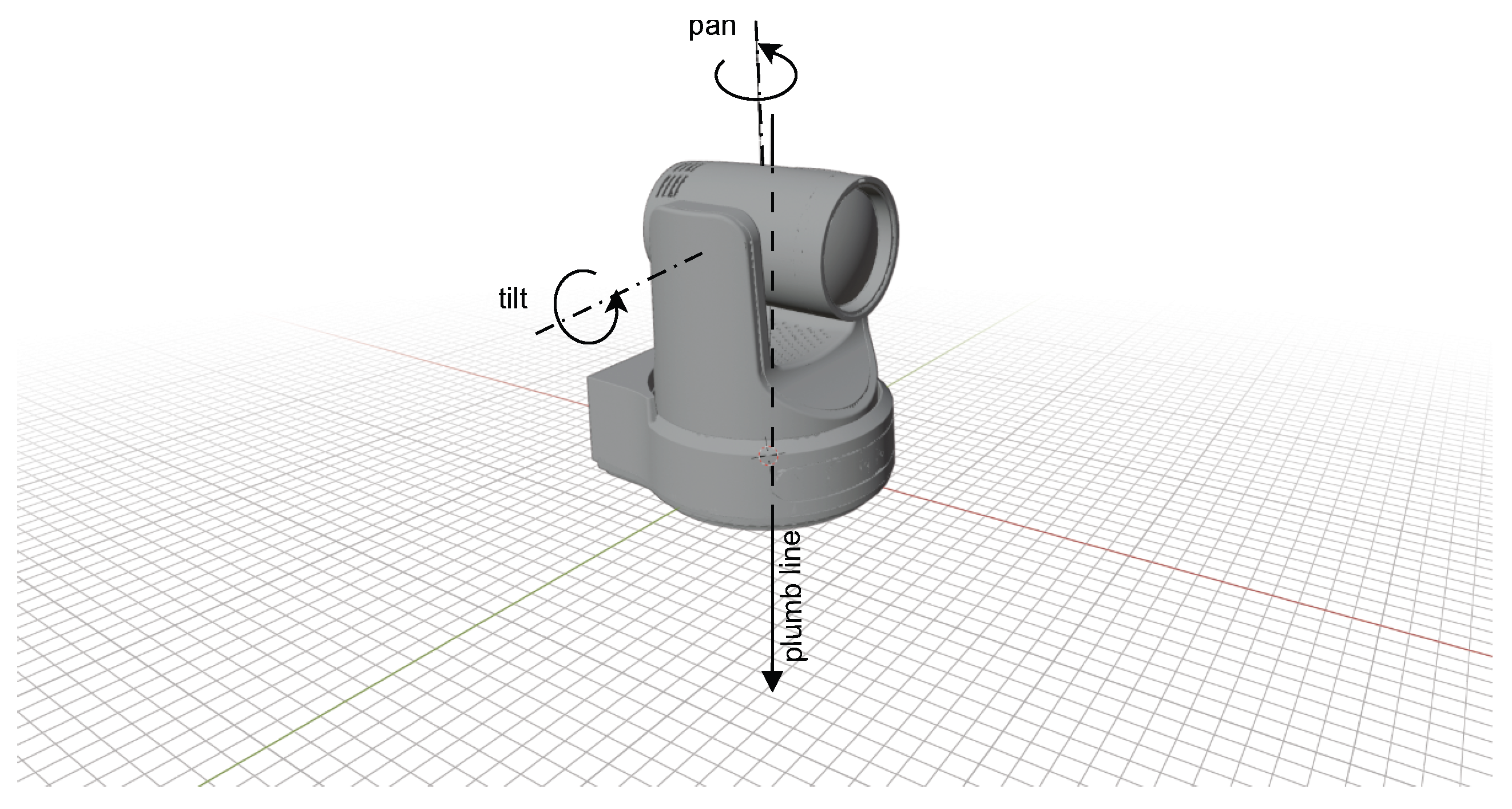
Figure 2.
The ENU et AER coordinate systems.
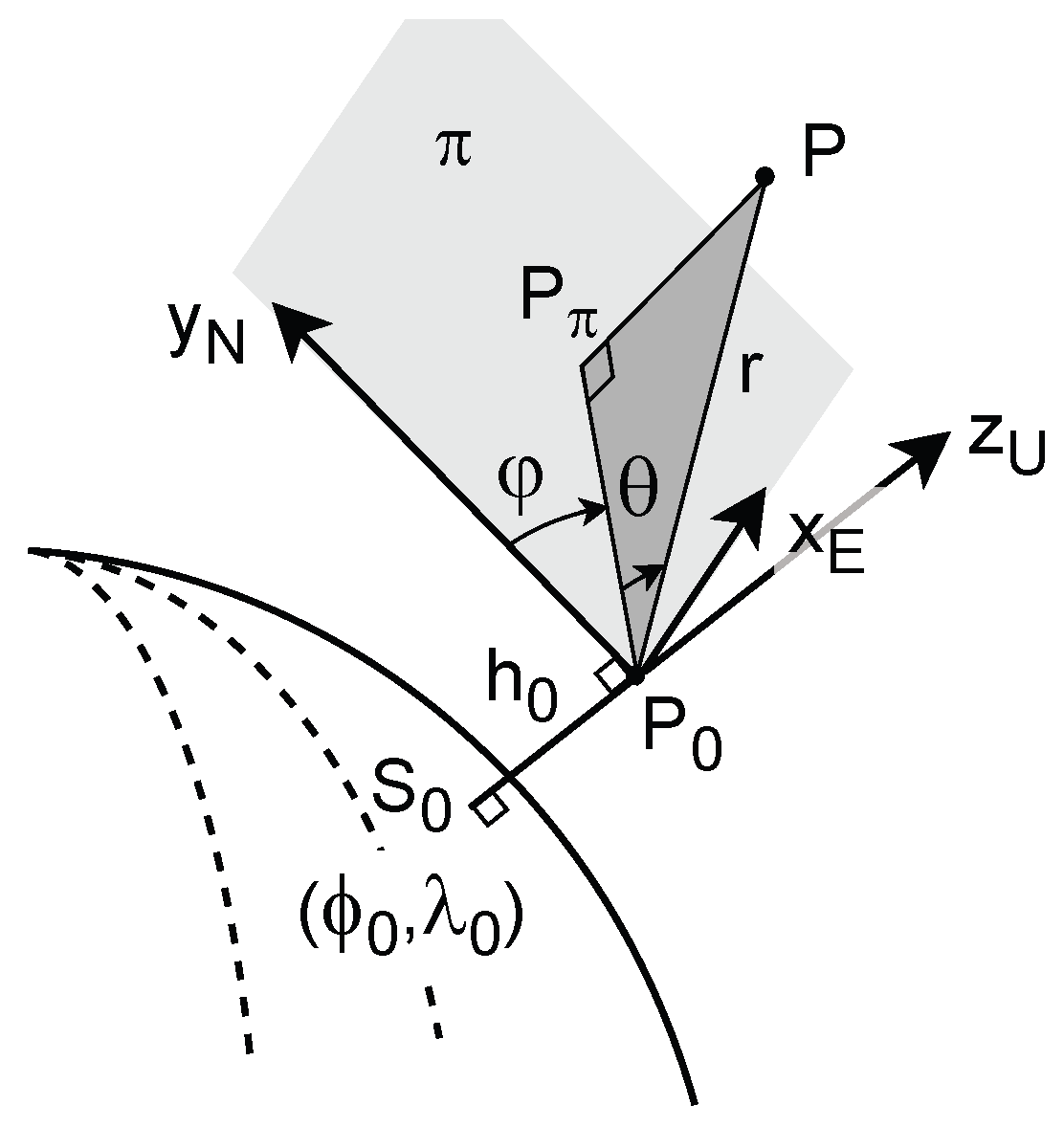
Figure 3.
Mapping from the 3D geometric space to the azimuth-elevation space.
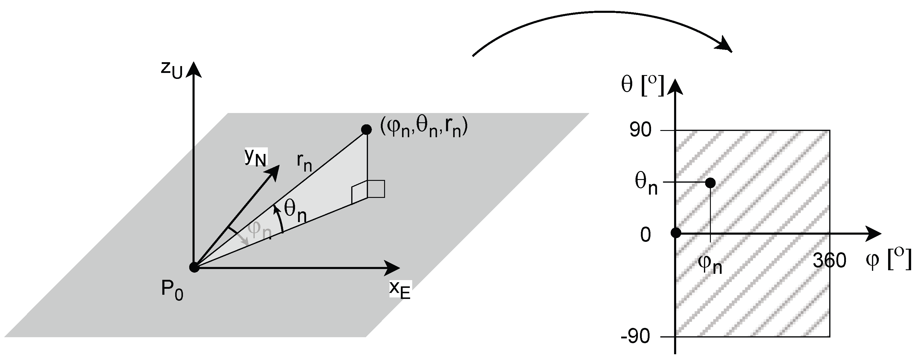
Figure 4.
LAEM of a surface.
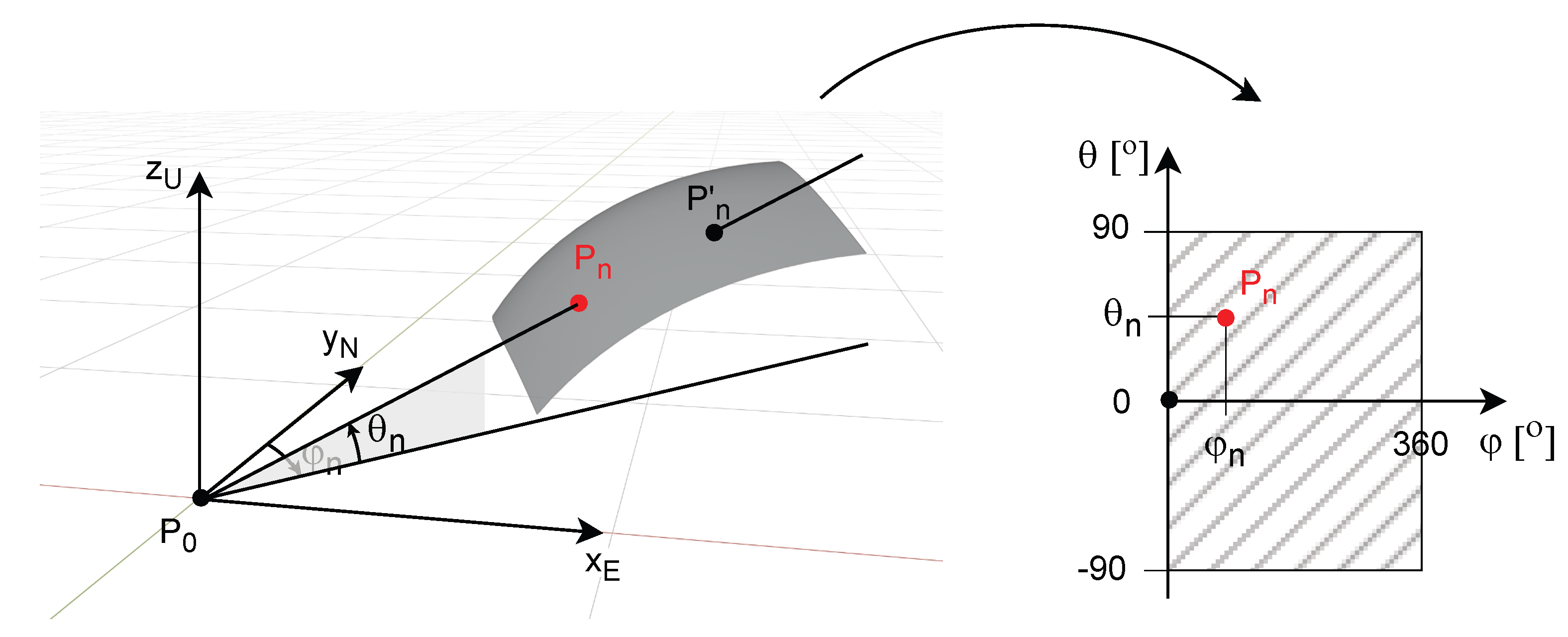
Figure 5.
Coordinates of the discrete LAEM.
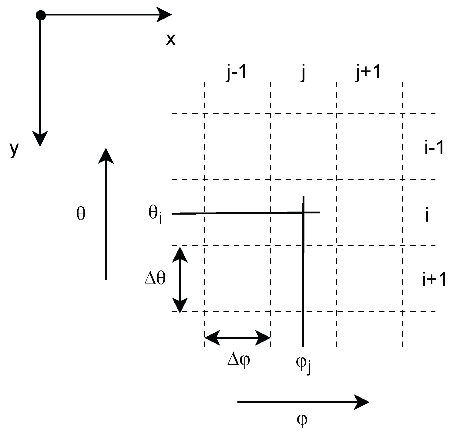
Figure 6.
Elementary surface patch used for DEM computation.
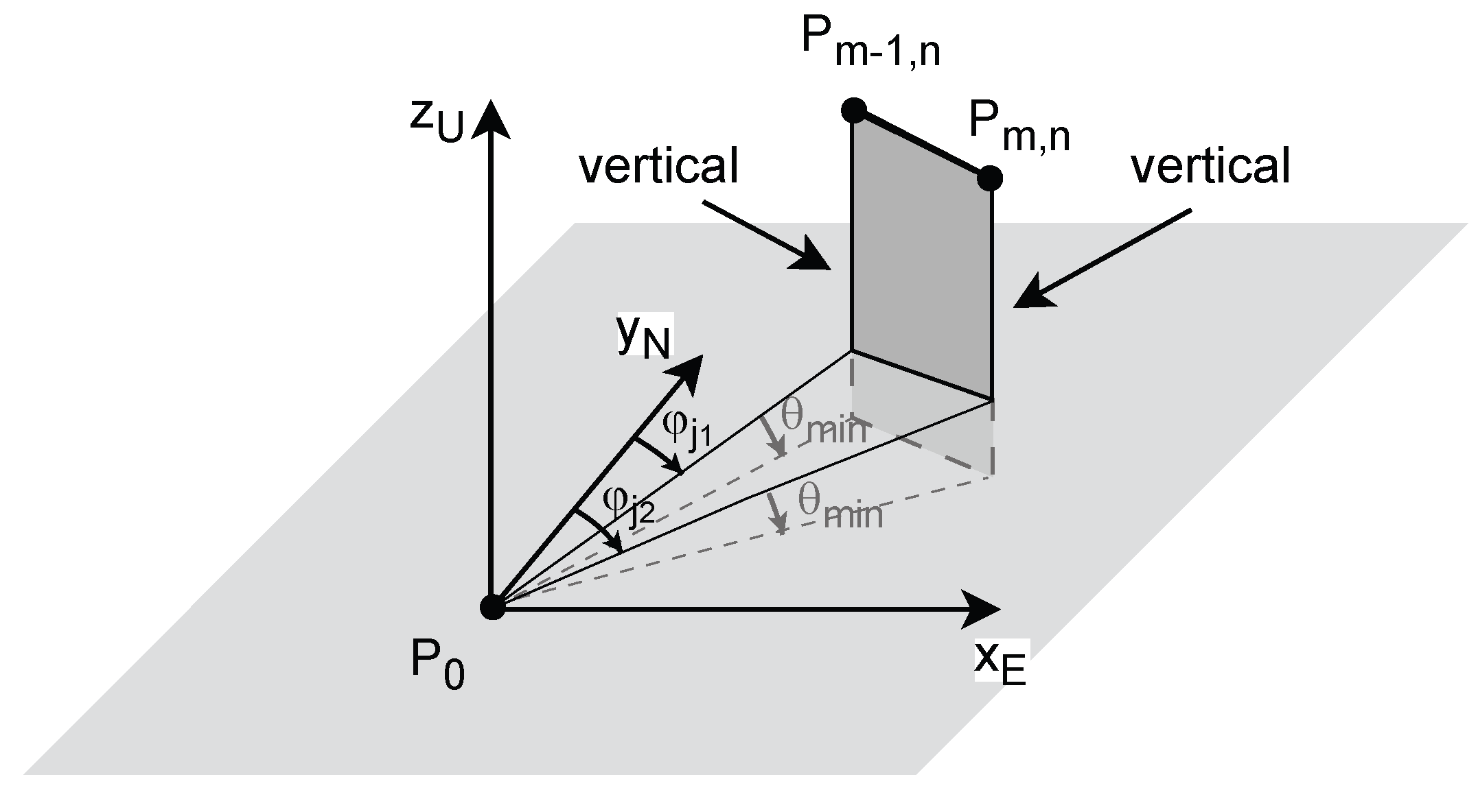
Figure 7.
DEM interpolation point at the discrete azimuth value .
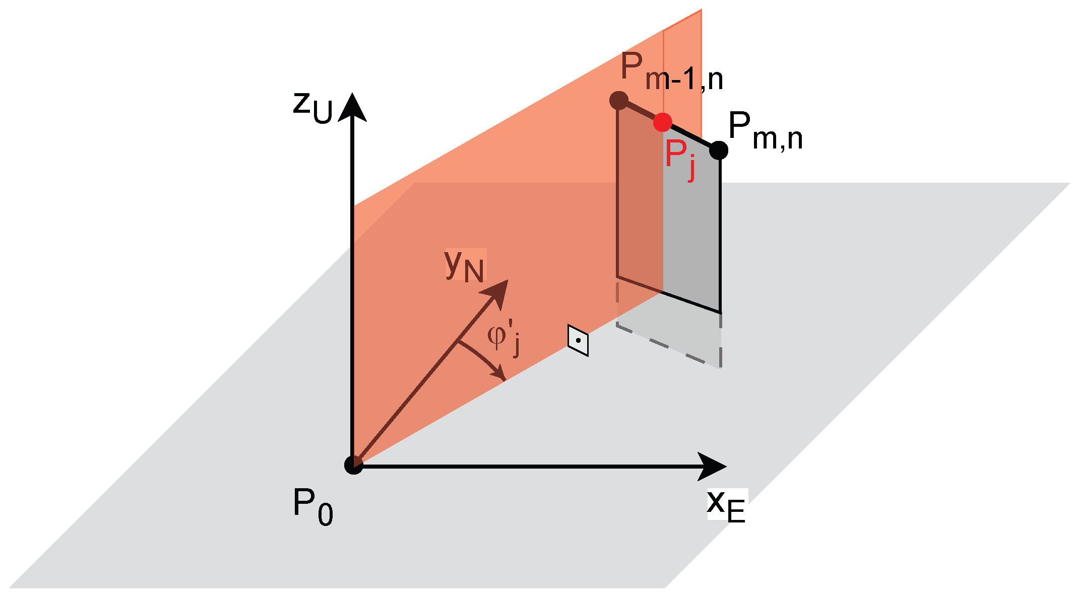
Figure 8.
Line from to the sphere centre C: (a) 3D view, (b) view in the plane .
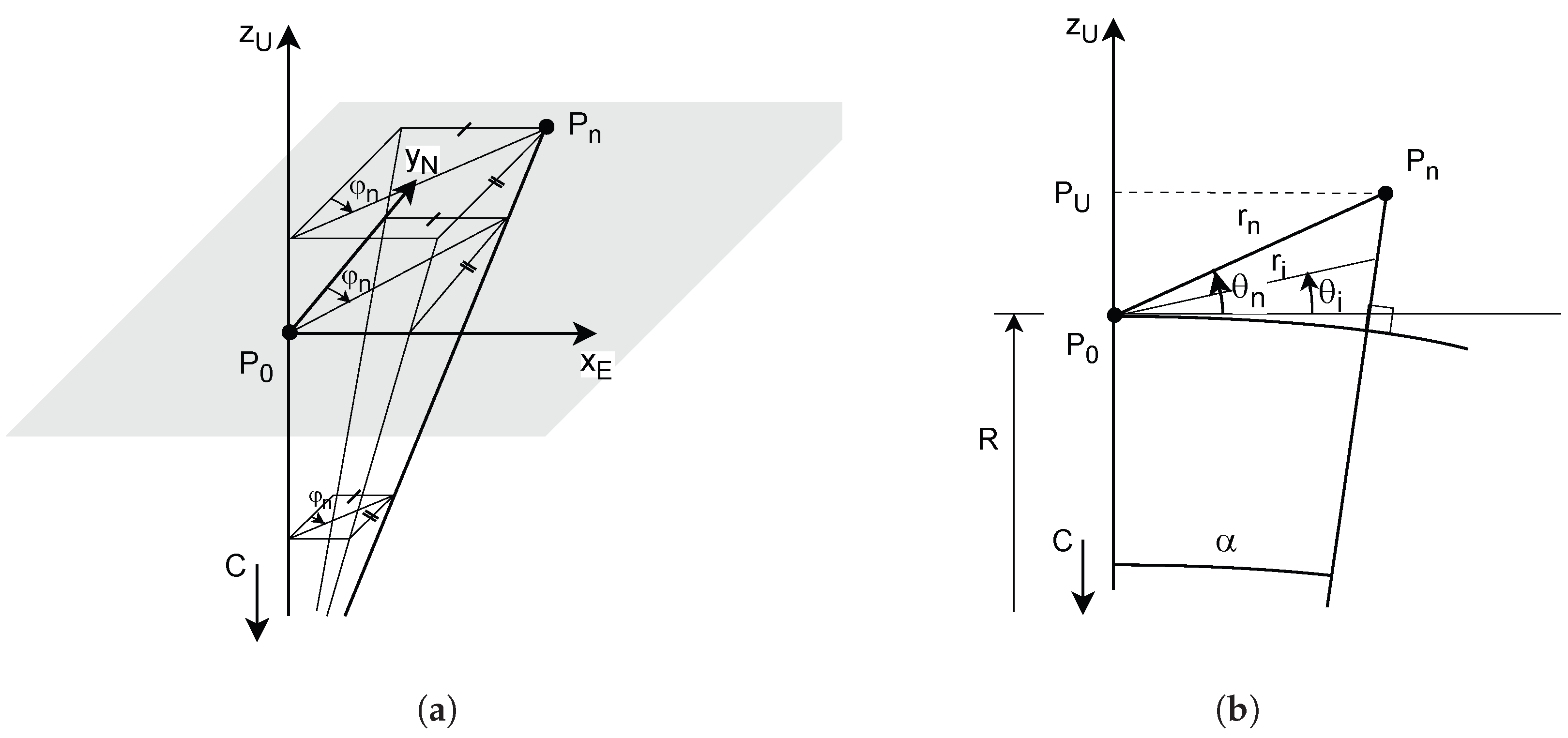
Figure 9.
Azimuthal and spatial resolution of the LAEM.
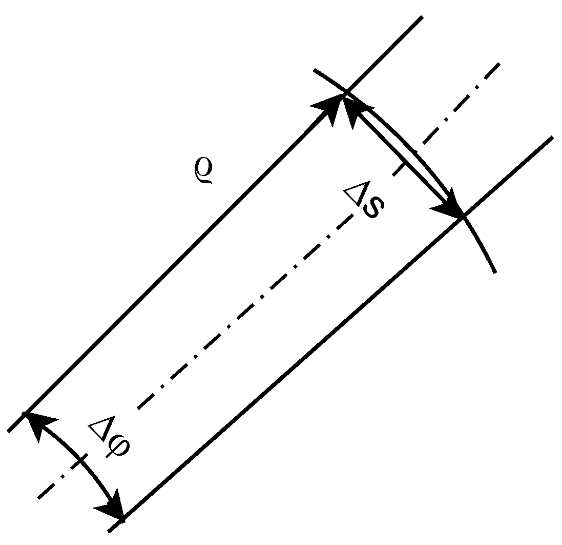
Figure 10.
LAEM variable spatial resolution compared to constant DEM resolution : (a) Close to the reference point. (b) Far from reference point.
Figure 10.
LAEM variable spatial resolution compared to constant DEM resolution : (a) Close to the reference point. (b) Far from reference point.
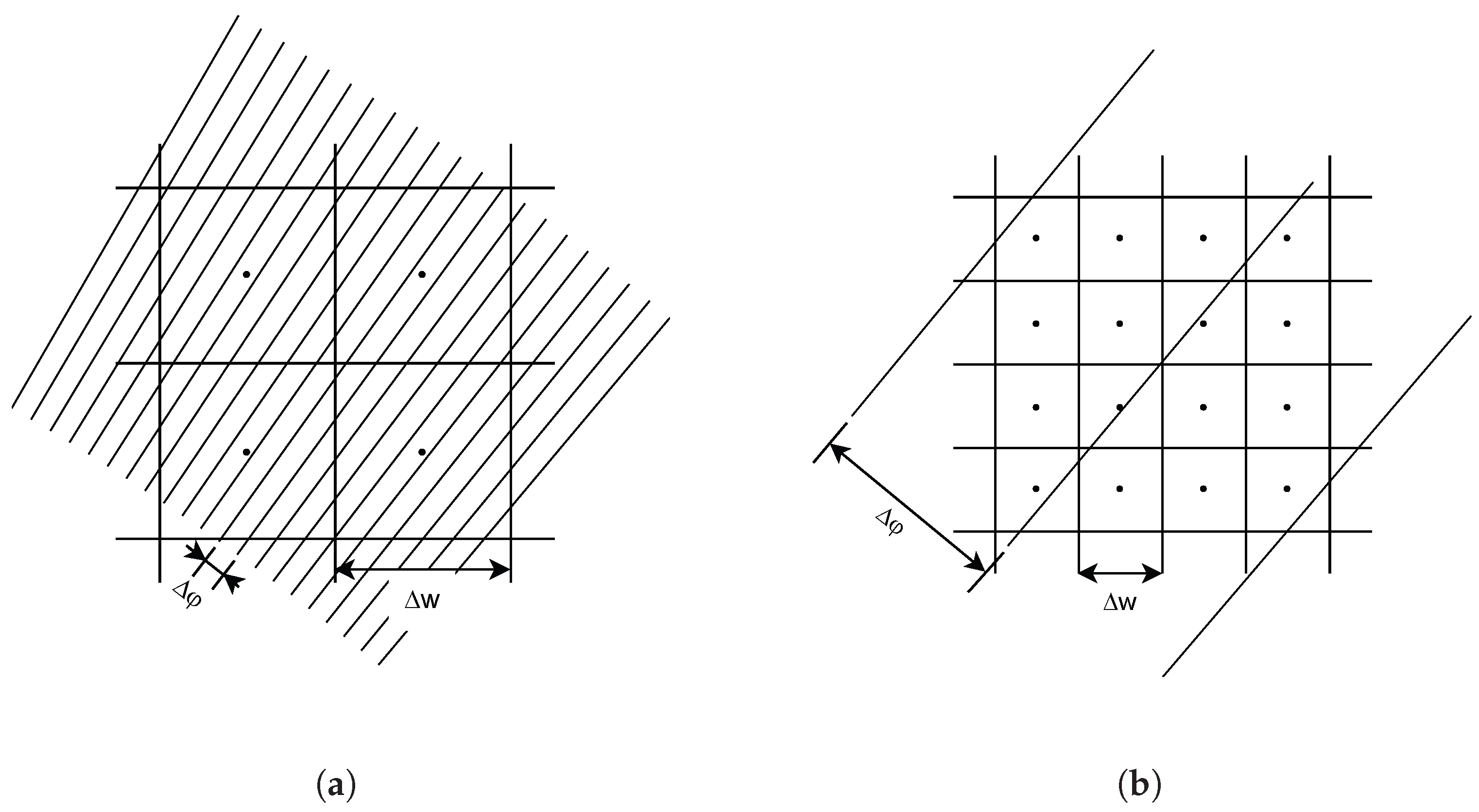
Figure 11.
Mechanical camera set-up: (a) View at distance. (b) Close view.
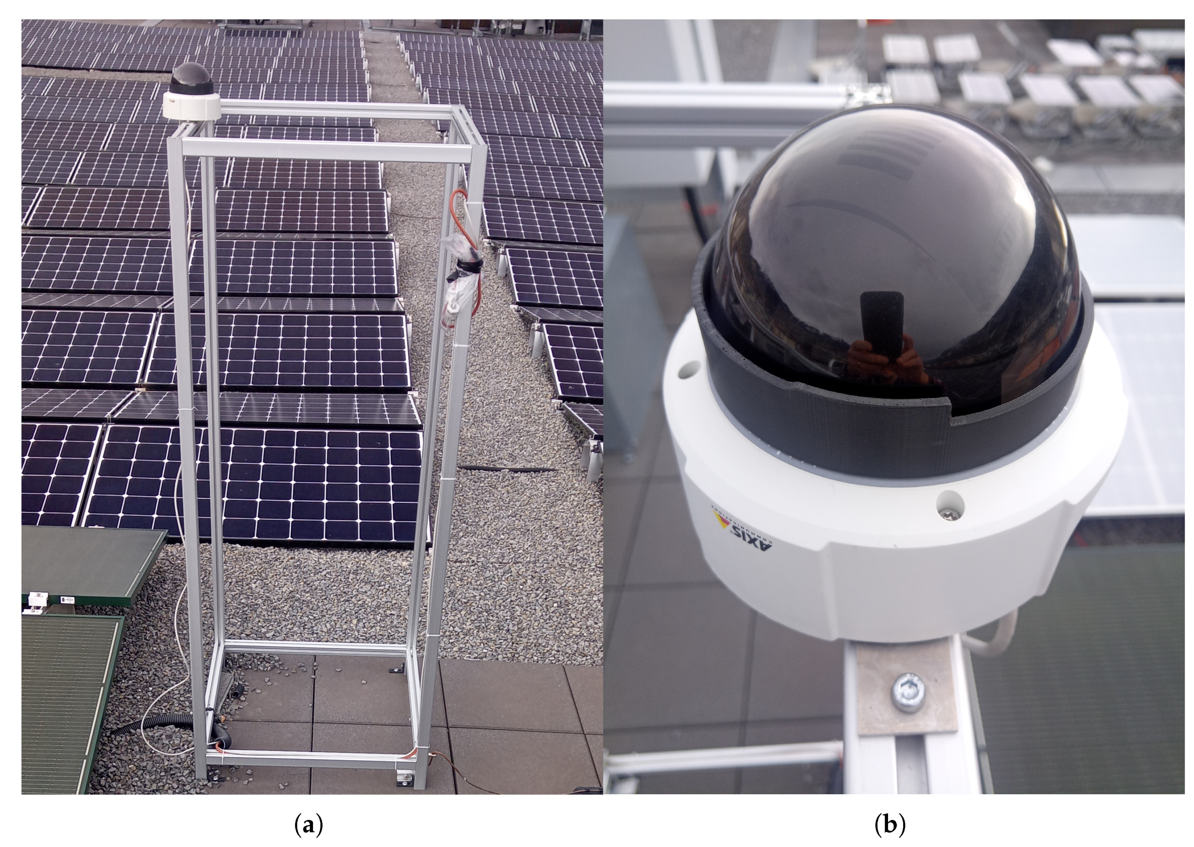
Figure 12.
Typical camera image in daylight and good weather.
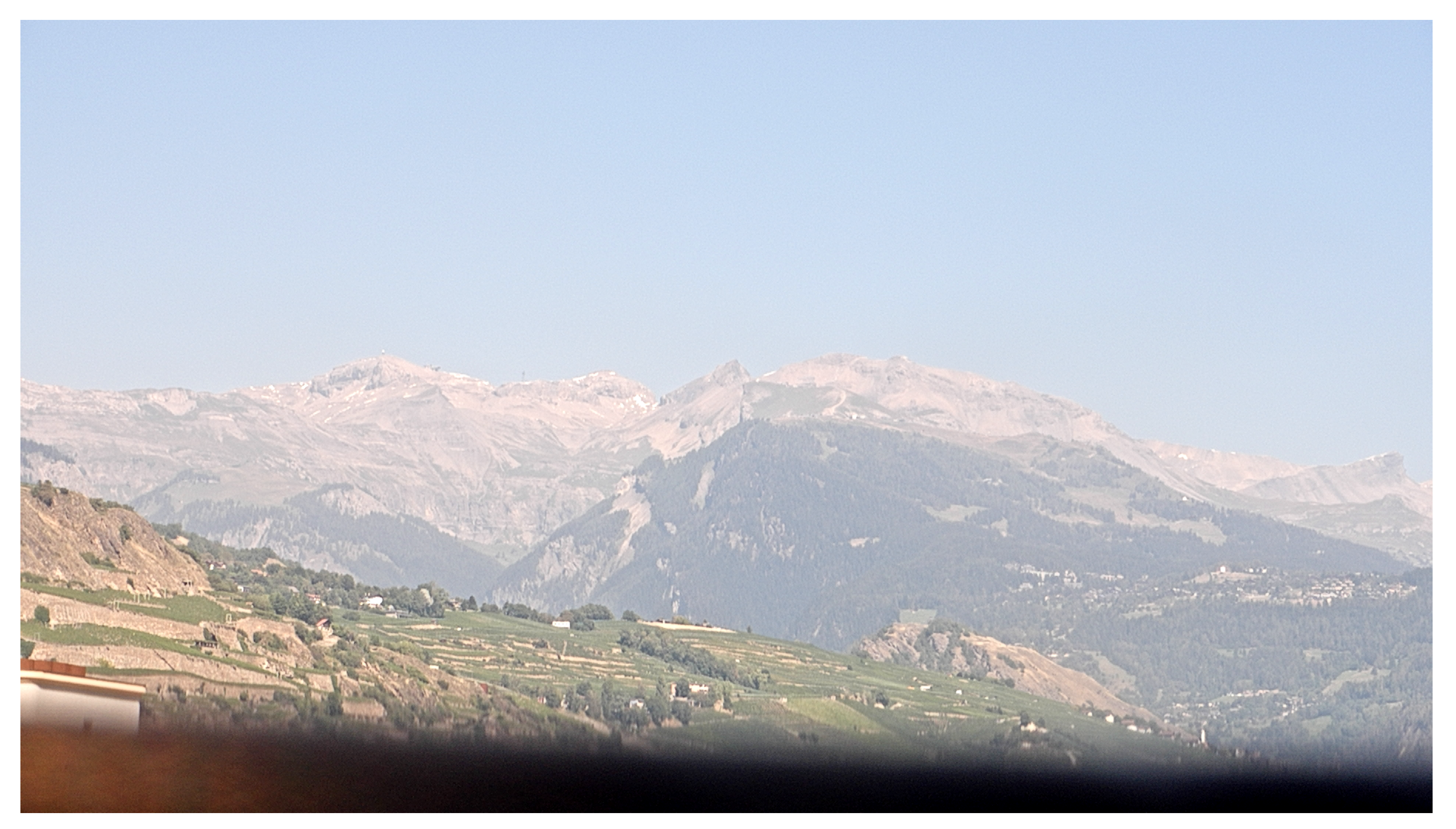
Figure 13.
Camera position from map.geo.admin.ch.
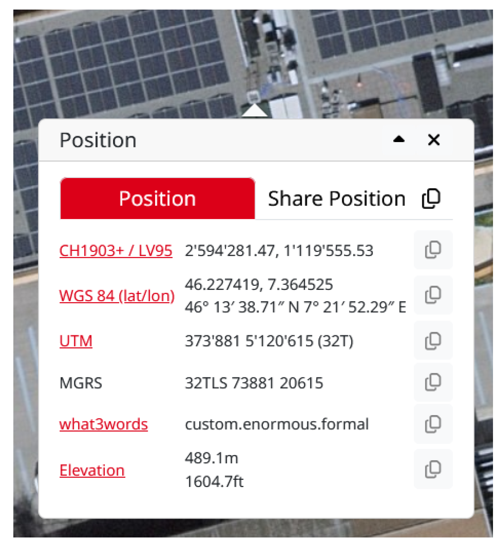
Figure 14.
Geosuite batch transform.
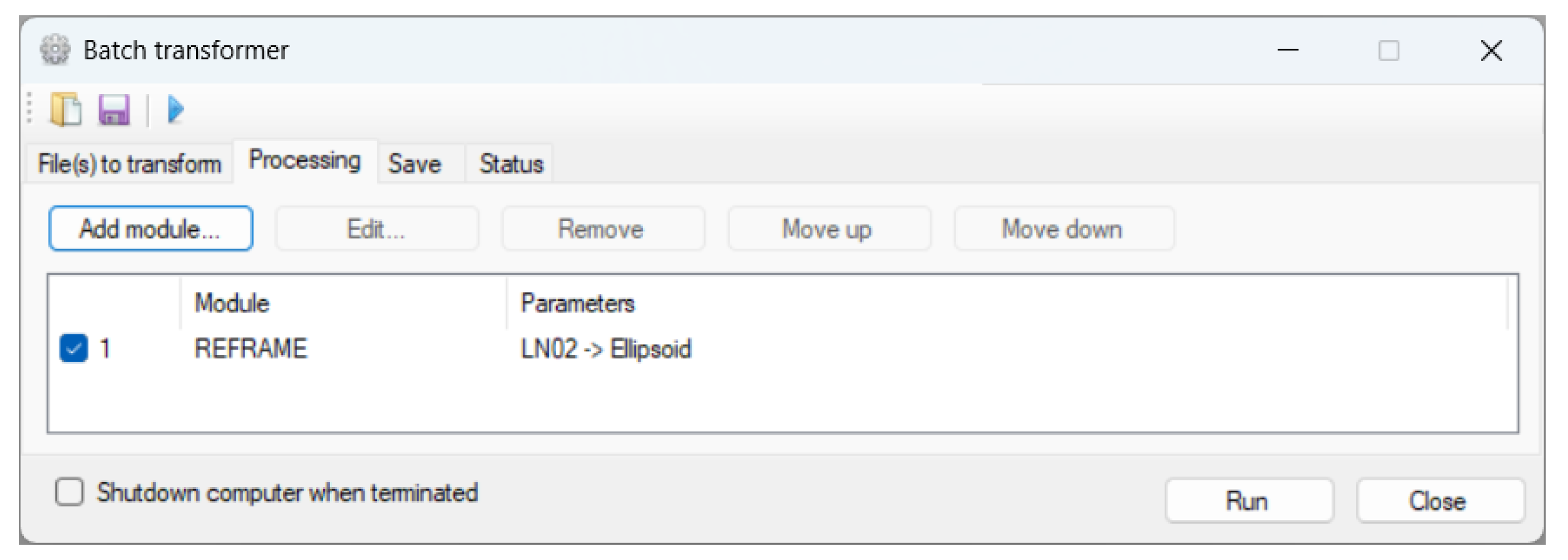
Figure 15.
Greyscale coded LAEM (the darker the lower the distance).
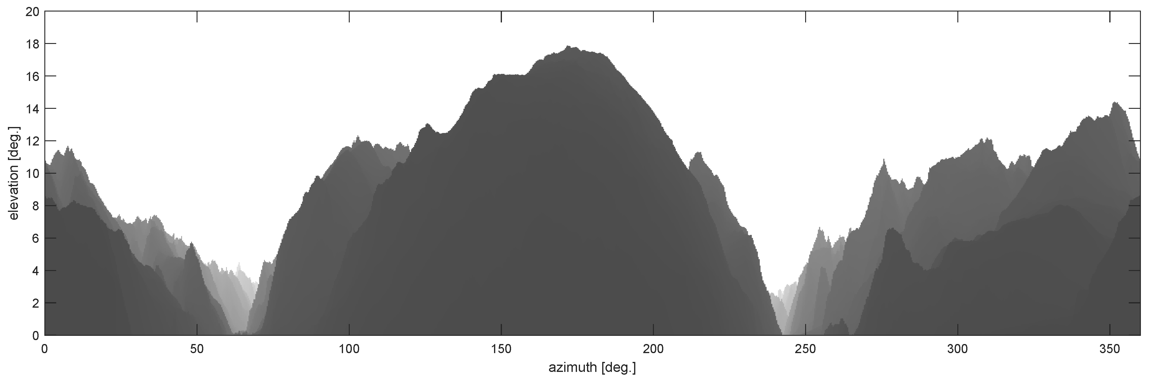
Figure 16.
Preselected and selected tiles.
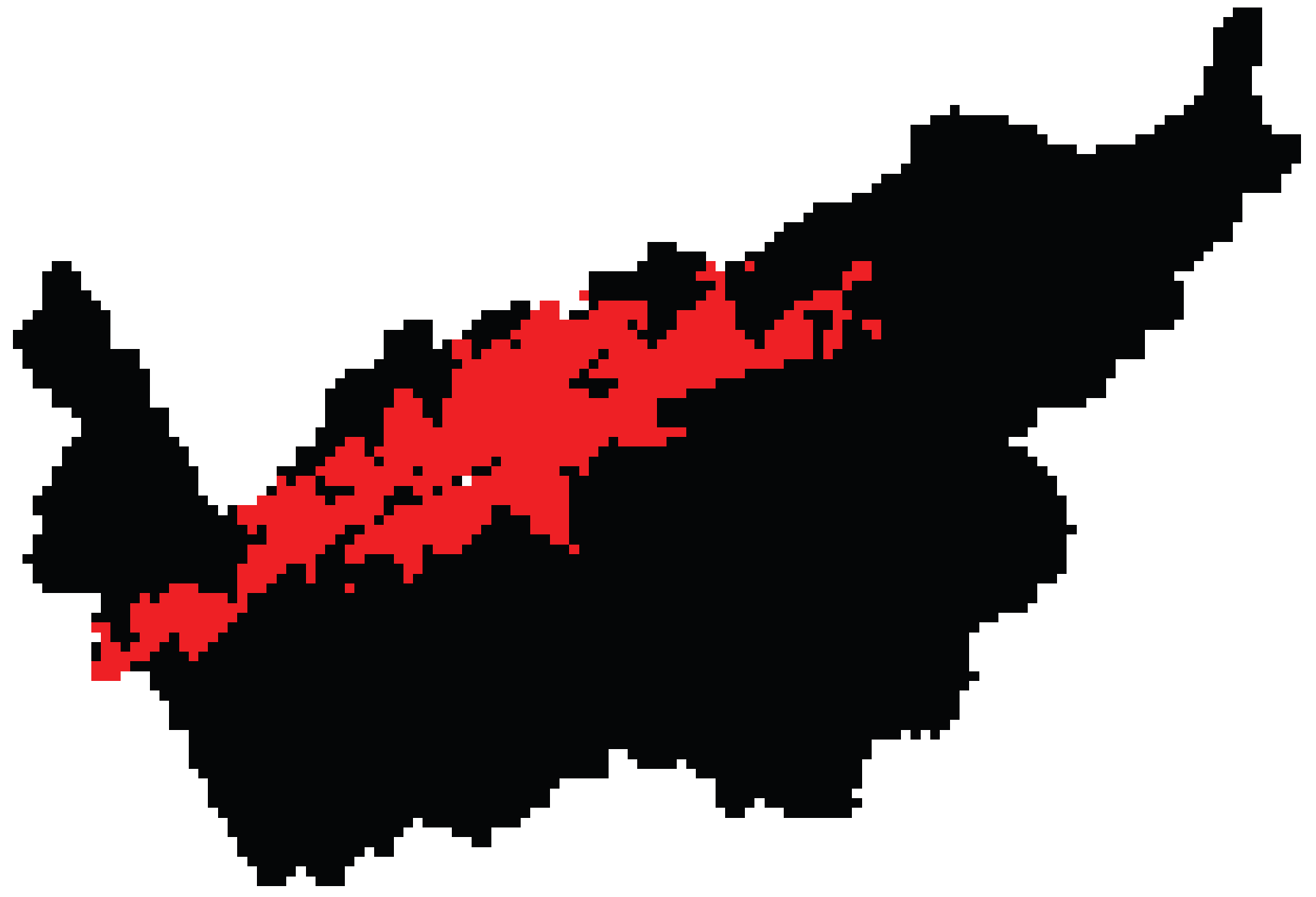

Table 1.
Estimated upper bound for the error in vertical direction on the GRS80 ellipsoid.
| planar approximation | spheric approximation | |
| d | ||
| 100 m | 0.000904 | 6.054193e-06 |
| 1 km | 0.009044 | 6.054193e-05 |
| 10 km | 0.090437 | 0.000605 |
| 100 km | 0.904294 | 0.006053 |
Disclaimer/Publisher’s Note: The statements, opinions and data contained in all publications are solely those of the individual author(s) and contributor(s) and not of MDPI and/or the editor(s). MDPI and/or the editor(s) disclaim responsibility for any injury to people or property resulting from any ideas, methods, instructions or products referred to in the content. |
© 2026 by the authors. Licensee MDPI, Basel, Switzerland. This article is an open access article distributed under the terms and conditions of the Creative Commons Attribution (CC BY) license (http://creativecommons.org/licenses/by/4.0/).
Copyright: This open access article is published under a Creative Commons CC BY 4.0 license, which permit the free download, distribution, and reuse, provided that the author and preprint are cited in any reuse.


