
Submitted:
02 January 2026
Posted:
06 January 2026
You are already at the latest version
Abstract
High-dimensional survival analyses require calibrated risk and honest uncertainty, but standard elastic-net Cox models yield only point estimates. We develop a fully Bayesian elastic-net Cox (BEN–Cox) modelfor high-dimensional proportional hazards regression that places a hierarchical global–local shrinkage prior on coefficients and performs full Bayesian inference via Hamiltonian Monte Carlo. We represent the elastic–net penalty as a global–local Gaussian scale mixture with hyperpriors that learn the ℓ1/ℓ2 trade-off, enabling adaptive sparsity that preserves correlated gene groups and, using HMC on the Cox partial likelihood, yields full posteriors for hazard ratios and patient-level survival curves. Methodologically, we formalize a Bayesian analogue of the elastic-net grouping effect at the posterior mode and establish posterior contraction under sparsity for the Cox partial likelihood, supporting the stability of the resulting risk scores. On the METABRIC breast-cancer cohort (n = 1 , 903; 440 gene-level features from an Illumina array with ≈ 24,000 gene-level features (probes)), BEN–Cox achieves slightly lower prediction error, higher discrimination, and better global calibration than a tuned ridge Cox baseline on a held-out test set. Posterior summaries provide credible intervals for hazard ratios, identify a compact gene panel that remains biologically plausible. BEN–Cox provides a theory-backed, uncertainty-aware alternative to tuned penalised Cox models, improving calibration and yielding an interpretable sparse signature in correlated, high-dimensional survival data
Keywords:
Bayesian elastic-net
; Cox proportional hazards
; high-dimensional survival
; shrinkage estimator
; posterior contraction
1. Introduction
Accurate time–to–event prediction guides decisions on therapy, follow-up, and trial eligibility. Modern molecular profiling yields wide, correlated predictor sets for comparatively modest cohorts, and in this high-dimensional regime Cox regression can become unstable and risk scores can miscalibrate. Penalised variants such as lasso, ridge, and the elastic–net stabilise estimation and encourage structure, yet they return only point estimates and depend on tuning, leaving uncertainty quantification and calibration largely ad hoc. This motivates a fully Bayesian formulation that delivers calibrated risk and honest uncertainty while respecting correlation among predictors.
The classical model for such time–to–event problems is the Cox proportional–hazards regression [1]. In its original form the model works well when the number of predictors p is small or at most moderate. Modern gene–expression studies, however, typically start from tens of thousands of microarray gene-level features measured on only a few thousand patients. In METABRIC, for example, the Illumina HT-12 v3 platform interrogates roughly gene features, but the publicly available cBioPortal file that we analyse here already provides gene–level summaries rather than raw feature intensities. After removing genes with missing values in this file we obtain gene-expression variables, and after the 10th–percentile variance filter we work with features (see Section 3). Thus, although the original assay is ultra–high–dimensional at the feature level, the resulting design matrix is still high–dimensional and strongly correlated relative to n, which makes the partial–likelihood surface relatively flat in many directions and the Cox estimates unstable.
One solution is to add penalties. The Lasso shrinks many coefficients exactly to zero, while ridge regression keeps all coefficients but pulls them toward zero. The elastic–net (EN) combines the two ideas and tends to keep groups of correlated genes together [2]. In addition, penalised Cox models have been widely used for high-dimensional survival and gene-expression data, including lasso and ridge-type penalties [3], as well as comparative studies and cross-validated prognostic pipelines for microarray cohorts [4]. More recently, post-shrinkage strategies have been proposed for high-dimensional Cox models [5]. Related to ridge-type regularisation, weighted ridge ideas and post-selection shrinkage strategies based on weighted ridge have also been developed; see Gao et al. [6] and the follow-up line of work on shrinkage and penalty estimation under censoring (see Hossain and Ahmed [7], Ahmed et al. [8]). Still, the elastic–net needs cross–validation to pick two tuning numbers and only returns point estimates, so we do not know how much uncertainty we have in each hazard ratio.
A key statistical motivation behind shrinkage is the bias–variance trade-off: in moderate-to-high dimensions, shrinking noisy estimates toward a central value can reduce mean squared error (see [9] for a modern post-shrinkage view in high-dimensional modeling). This is not only a heuristic idea: the Stein-type shrinkage approach shows that, for multivariate normal means in dimension , the usual unbiased estimator can be inadmissible and can be improved by shrinkage estimators. The same principle underlies many regression shrinkage methods. In particular, ridge regression can be interpreted as a Bayes estimator under a Gaussian prior, and many Stein-type and empirical Bayes procedures choose the shrinkage intensity by estimating hyperparameters from data. In this sense, modern penalised survival models sit very close to empirical Bayes thinking, even when they are presented as optimisation-based methods. The BEN–Cox model developed here follows this idea directly: the shrinkage strengths are treated as unknown and learned from the data via hyperpriors, providing a principled Bayesian analogue of data-driven shrinkage.
Bayesian thinking treats a penalty as the negative log of a prior. A Laplace prior gives the Bayesian Lasso [10], and mixing a Laplace with a Gaussian prior gives the Bayesian elastic–net (BEN) [11,12]. Putting hyper–priors on the mixing scales lets the data decide how much and shrinkage to apply, and posterior samples provide full credible intervals. Recent theory also shows that such scale–mixture priors contract toward the truth at near-optimal rates under sparsity [13].
In this paper we fit a fully Bayesian EN Cox model to the METABRIC cohort (, gene–level features derived from an original –probe array). Our aims are to
- show that Hamiltonian Monte Carlo can draw stable posterior samples in a correlated, high–dimensional survival setting,
- compare predictive accuracy, discrimination, and calibration against a tuned ridge Cox baseline, and
- check that the genes kept by the model contain known biology, for example the PAM50 signature first reported in Curtis et al. [14],
- and, importantly, provide theoretical justification for the BEN–Cox in which we formalize a Bayesian elastic–net grouping effect and a posterior contraction result under sparsity (see Section 2.5 and Appendix A).
The rest of this article is organised as follows. Section 2 introduces the proposed BEN–Cox model, prior specification, and theoretical properties. Section 3 describes the METABRIC data set and the pre-processing procedure. Section 4 presents the application results, including predictive performance metrics and calibration diagnostics based on Demler et al. [15]. Section 5 discusses implications and limitations of the proposed method, and Section 6 provides concluding remarks.
2. Methodology
2.1. Model Specification
For patient , let denote the observed data, where represents the follow-up time, is the event indicator ( if the event is fully observed and if the event time is right-censored), and is a p-dimensional vector of z-standardized -transformed gene expression feature intensities. Here, denotes the base-2 logarithm, corresponding to the conventional transformation applied to raw expression intensity measurements. The Cox proportional hazards model [1] assumes
with unspecified baseline hazard . Inference uses the log partial likelihood
When p is large and predictors are strongly correlated, regularisation is essential; more generally, the same framework covers regimes where p may grow with n.
2.2. Bayesian Elastic–Net Prior
We place an elastic–net prior on that unifies and shrinkage:
recovering lasso and ridge as or [2]. For computation we use the normal–exponential mixture for the Laplace part with a Gaussian ridge factor:
which integrates back to (3). We use weakly-informative global hyperpriors,
so the balance is learned from the data. The part promotes sparsity; the part stabilises groups of correlated features (useful for gene modules).
2.3. Posterior Distribution
Let . Up to normalising constants, the joint posterior is
Because the Cox likelihood is non-conjugate, we use Hamiltonian Monte Carlo for full Bayesian inference.
2.4. Hamiltonian Monte Carlo Inference
We fit the model with the No-U-Turn Sampler [16,17]. The parameter block is
and the target potential uses (2) and (4). We run four chains, warm up to adapt step size and diagonal metric, then draw posterior samples. Convergence is assessed with and effective sample size thresholds; energy/BFMI diagnostics are checked for geometry pathologies. Posterior predictive survival uses Breslow’s estimator per draw. In this context, let denote the distinct ordered event times in the sample, let be the number of events at time , and define the risk set . Then Breslow’s estimator at posterior draw m is given by
Before turning to the theoretical properties, we briefly summarise how the proposed procedure works. Figure 1 shows a DAG of the approach, highlighting the parameters used in the model and their probabilistic relationships.
In Figure 1, HC(0,5) is a Half-Cauchy hyperpriors with scale 5, providing weakly informative priors for the global shrinkage parameters and , as specified in (5). is a global penalty parameter controlling the degree of sparsity in the elastic–net prior; learned from the data via the Half-Cauchy(0,5) hyperprior and typically scaling as in high-dimensional regimes. is again a global penalty parameter controlling ridge regularization strength; keeping ensures posterior propriety and stabilizes HMC sampling. is latent exponential scale variables with , enabling the normal–exponential mixture representation of the Laplace component of the elastic–net prior in (4). is regression coefficient for the j-th gene-expression feature (covariate ); conditionally Gaussian given and , with , as in (4). is unspecified baseline hazard function in the Cox model (1); estimated post hoc via Breslow’s estimator at each posterior draw. is our linear predictor for subject i and , representing the log hazard ratio in (1). : p-dimensional vector of z-scored gene-expression measurements for subject i, pre-processed as described in Section 3.4. Finally, is a observed survival time for subject i possibly right censored and is as known event indicator, with if death is observed and if the observation is right-censored at time .
2.5. Theoretical Properties
This section summarizes the theoretical properties for the introduced BEN–Cox approach. In particular, Theorem 1 gives a Bayesian analogue of the elastic-net grouping idea at the posterior mode, and Theorem 2 establishes posterior contraction under sparsity. A complete proof of Theorem 2 including test construction, prior mass, and entropy bounds in the Cox partial-likelihood setting is provided in Appendix A. In this context we use the following notation: is the norm; is the identity matrix; is the Cox risk set. In addition, are the observed partial-likelihood information. Posterior is under (3)–(4). Also the following assumptions are needed to ensure the theoretical soundness.
Assumptions
- (A1)
- Columns of are z-scored on the training split; and entries are bounded.
- (A2)
- As a Cox model regularity condition, event times lie in a compact interval and the baseline hazard is locally bounded; is twice continuously differentiable (see [1]).
- (A3)
- There exists such that for all v with support S, , in a neighbourhood of .
- (A4)
- As a sparsity assumption, the truth is –sparse with .
- (A5)
We can explain the details of assumptions individually as follows: (A1) standardizes columns so correlation and curvature arguments are interpretable and avoids scale pathologies in HMC, which is crucial for Bayesian inference. When it comes to (A2), it is the usual smoothness condition that guarantees a well-behaved partial likelihood. (A3) is the high-dimensional analogue of identifiability: restricted curvature prevents flat directions on sparse supports, which can be interpreted as the Cox counterpart of restricted eigenvalues. (A4) encodes the high-dimensional regime with effective dimensionality ; it is the minimal condition for rates and finally (A5) ensures the prior places enough mass near the optimal scale while keeping so the geometry is strongly convex and the posterior proper.
In the following two basic geometric properties are introduced that we will use repeatedly: (i) the concavity of the Cox partial likelihood, which controls the curvature of the log-posterior, and (ii) the mixture representation of the elastic–net prior, which links our hierarchical formulation (4) back to the penalty in (3). These results are standard, but they are provided for completeness.
Lemma 1
Lemma 2.
With the Gaussian ridge factor controls the tails in all directions. Since is concave (see Lemma 1) and the hyperpriors are proper according to assumption A5, the posterior normalizes. Moreover, is strongly convex with curvature , so the posterior mode in is unique. Therefore, this stabilizes the optimization and HMC geometry.
With these building blocks in place, we now formalise two behaviours that are particularly relevant in our high-dimensional gene-expression setting. First, the grouping effect shows that highly correlated gene features tend to receive similar coefficients, so the model naturally picks gene modules rather than arbitrary single gene features. Second, a contraction result shows that, under sparsity, the BEN–Cox posterior concentrates around the true coefficient vector at the usual high-dimensional rate, providing reassurance that our calibrated risk scores are statistically well behaved as n grows. We state a grouping theorem for the posterior mode, followed by a contraction theorem for the full posterior.
Theorem 1
(Bayesian elastic–net grouping at the posterior mode). Assume (A1)–(A2). Let be the posterior mode under (3) with fixed and . For standardized columns with sample correlation ,
In particular, if and remains bounded, then . Hence the difference tends to zero (Bayesian analogue of the ElasticNet’s grouping effect; see Zou and Hastie [2], Hans [12]).
Proof.
Consider . Karush–Kuhn–Tucker (KKT) conditions give with . Taking the j–k difference,
so For the score difference, express the Cox score using risk-set weights and apply Cauchy–Schwarz to the difference column . With standardisation (A1), , yielding Scaling per observation and absorbing gives the stated bound with . If and is not diverging, the difference vanishes. Since the posterior typically concentrates in a neighborhood of under standard regularity, the grouping behavior at the mode is often reflected in posterior summaries as well; we observe this empirically in the METABRIC analysis. □
Since the posterior distribution is (locally) log-concave and concentrates around , the grouping effect at the mode also appears in posterior means. In other words, highly correlated gene features tend to have similar posterior mean coefficients as well; see Li and Lin [11], Hans [12] for related results on Bayesian elastic–net concentration.
Theorem 2.
(Posterior contraction). Assume (A1)–(A5) and let . Then there exists such that
This theorem is a posterior contraction result: as n grows, the BEN–Cox posterior for concentrates inside an –ball of radius around the sparse truth . The proof follows the standard Bayesian contraction arguments of Ghosal and van der Vaart [13], adapted to the Cox partial-likelihood setting, and combines three ingredients. (i) Tests: Assumption (A3) provides local quadratic lower bounds for , which yield exponential tests that separate from the complement of an –ball of radius . (ii) Prior mass: By Lemma 2 and (A5), the prior allocates at least mass to such balls (taking and using to stabilize curvature). (iii) Complexity: The class of –sparse vectors within radius has logarithmic complexity of order , which is dominated by . A complete, proof specialised to our Cox partial-likelihood setting (including the testing argument and the hyperprior treatment) is given in Appendix A.
Under Assumptions (A1)–(A4) and the contraction result in Theorem 2, the posterior for concentrates around the true pair . The survival function is continuous in on compact time intervals, and Breslow’s estimator is uniformly consistent for the baseline cumulative hazard in the Cox model [19]. Combining these facts, one can obtain:
for any fixed covariate vector and finite horizon . In other words, the posterior predictive survival curves converge to the true survival function uniformly on compact time intervals.
From a computational point of view, the ridge component with induces strong convexity in , while the z-scaling in (A1) keeps the design entries bounded. [16,17].
For practical implementation, it is helpful to summarize the full BEN–Cox workflow from raw gene-expression data to posterior summaries and predictive metrics. The following step-by-step algorithm makes explicit how the model, prior, MCMC inference, and evaluation pieces fit together in our analysis.
3. Data
3.1. Cohort Description
We analyse the Molecular Taxonomy of Breast Cancer International Consortium (METABRIC) cohort [14,20]. The study combines tumours from two centres (Cambridge, UK and Vancouver, Canada) and is publicly available through the cBioPortal interface [21]. The dataset contains clinical variables, overall survival, and a gene–expression matrix. From this file we extract overall survival and gene–expression information and remove subjects with missing survival time or status. After this quality control step we retain primary invasive breast cancers for our analysis.
3.2. Outcome
The time–to–event end-point is overall survival (OS). In the cBioPortal file OS is reported in months; we convert this to days for the modelling step and define the event indicator for deaths and for right-censored observations. Among the 1903 subjects, 800 experience the event (42.0 %), and the median follow-up is approximately 16.4 years, estimated using the reverse Kaplan–Meier method.
3.3. Predictors
- Gene expression : The METABRIC dataset provides Illumina HT-12 v3 micro-array measurements summarised at the gene level. In the version used here this block contains gene–expression features, indexed from the BRCA1 gene onwards. While the original METABRIC platform measures many more micro-array gene-level features, we restrict attention to this gene-level expression matrix for a more stable and reproducible design.
- Clinical covariates : age at diagnosis, tumour size, histological grade, lymph-node status and treatment indicators (hormone/chemotherapy) are also available in the downloaded dataset. These variables are not used in the present study but are retained for potential future work and for possible extensions of the BEN–Cox model.
3.4. Preprocessing
We first remove genes whose variance lies below the 10th percentile across patients, leaving gene–expression features. This variance filter removes almost-constant gene features and improves the conditioning of the design matrix. The data are then split once into an 80 % training set and a 20 % test set, stratified by the event indicator so that the censoring fraction is similar in both splits. Each gene is z-scored in the training set to have mean 0 and variance 1, and the same centring and scaling are applied to the test set. Finally, the survival tuples are encoded as described in Section 2.1, with measured in days and the event indicator.
4. Application
4.1. Experimental Design
We treat METABRIC as a single large cohort and mimic a typical prognostic modelling workflow: a model is fitted once on a development set and then evaluated on a separate test set. The data are therefore split once into 80 % training and 20 % testing, stratified on the event indicator so that the proportion of deaths and censored observations remains comparable across the two splits.
All tuning and model fitting are performed using only the training data. For the ridge-penalised Cox baseline we use five-fold cross-validation to select the penalty parameter , with the concordance index as the optimisation criterion. In contrast, the Bayesian elastic-net Cox (BEN–Cox) model treats the elastic–net penalties as random: the global shrinkage parameters follow Half-Cauchy hyperpriors and are learned jointly with the regression coefficients. This avoids an additional tuning loop and lets the data determine the balance between and shrinkage.
Posterior inference for BEN–Cox relies on Hamiltonian Monte Carlo as implemented in Stan, using the No-U-Turn Sampler (NUTS) with adaptively tuned step size and diagonal mass matrix. Starting from zero coefficients and diffuse initial values for , the chain is run until trace plots stabilise and effective sample sizes for the regression coefficients are comfortably above standard thresholds. The initial part of the chain is discarded as warm-up, and all posterior summaries are based on the retained draws. In particular, we monitor mixing and autocorrelation for representative coefficients and for the global shrinkage parameters to ensure that the posterior exploration is adequate for downstream prediction and uncertainty quantification.
4.2. Baseline Models
To show the BEN–Cox model’s advantages and disadvantages and how well it performs, we compare it against two baseline Cox models:
- Null Cox: a Cox model with no gene-expression covariates, i.e., all subjects share the same baseline hazard (no covariate effects). This provides a no-information baseline for discrimination and absolute-risk calibration.
- Ridge Cox : an -penalised Cox model fitted with glmnet, where the penalty is chosen by five-fold cross-validation on the training set. This is a natural frequentist benchmark for high-dimensional survival modelling when sparsity is not enforced explicitly.
Also note that, all models are fitted on exactly the same training data and are evaluated on the same held-out test set.
4.3. Evaluation Metrics
We assess predictive performance along three ways: time-dependent prediction error, discrimination between subjects with different risk, and calibration of predicted survival probabilities.
Let denote the true event time for patient i, the censoring time, and the observed time, with the event indicator. For a given model, let be the predicted survival probability at time t for patient i, and let be its linear predictor or risk score.
As mentioned in the Algorithm 1, we have 3 main performance metrics that are IBS, C-index and calibration slope and metrics. These metrics are defined as follows:
| Algorithm 1: BEN–Cox pipeline |
| Input: gene matrix , times , events . |
| Output: posterior draws , test-set performance metrics. |
| 1. Pre-processing |
| 1.1 Remove gene-level features whose variance is below the 10th percentile [14]. |
| 1.2 z-score each column of using training-set moments. |
| 2. Train–test split |
| 2.1 Randomly split subjects 80/20 into training and test sets, stratified by . |
| 2.2 Fix the random seed and record the split for reproducibility. |
| 3. Model and prior |
| 3.1 Specify the Cox model (1) with elastic–net prior (3). |
| 3.2 Use the normal–exponential mixture representation (4) and |
| Half-Cauchy hyperpriors for as in (5). |
| 4. HMC sampling with Stan (training set only) |
| 4.1 Fit the model using 4 chains, warm-up + sampling. |
| 4.2 Check convergence: and ESS for all coefficients. |
| 4.3 Retain posterior draws and, for each draw, compute |
| the Breslow baseline cumulative hazard . |
| 5. Prediction on the test set |
| 5.1 For each test subject i and draw m, compute |
| linear predictor and |
| survival curve . |
| 5.2 Form posterior summaries (e.g., mean or median survival probabilities). |
| 6. Performance metrics (test set) |
| 6.1 Compute the integrated Brier score (IBS). |
| 6.2 Compute the concordance index (C-index) for discrimination. |
| 6.3 Compute calibration slope and intercept, following Demler et al. [15]. |
Integrated Brier Score:
The Brier score at time t is a squared prediction error adapted to the survival setting. Following the inverse-probability-of-censoring weighting (IPCW) approach, we write
where is an estimate of the censoring survival function (e.g. Kaplan–Meier for ). Intuitively, patients who are still under follow-up at time t contribute squared error for predicting survival, and patients who die before t contribute squared error for predicting death, with both contributions reweighted to account for censoring.
To summarize performance over a time window we use the integrated Brier score (IBS),
which can be interpreted as a time-averaged mean squared prediction error for survival probabilities up to horizon . In practice we approximate the integral numerically on a fine grid of time points.
Concordance (C) Index:
Discrimination is quantified using Harrell’s concordance index (C-index). The C-index estimates the probability that, for a randomly chosen pair of comparable patients , the one who dies first also has the higher predicted risk. Formally,
where the denominator counts all comparable pairs (those with an observed event before the other’s follow-up has finished) and the numerator counts how often the model orders their risk correctly.
Grouped Calibration (GND ):
In addition to the calibration slope and intercept, we also report a Greenwood–Nam–D’Agostino (GND) type grouped-calibration chi-square type statistic [15] as a global calibration measure. To achieve that we consider, which means a fixed, clinically relevant follow-up time (in this study, horizon years), and we only look at whether each patient has experienced the event before this time or not.
For each patient we define a horizon event indicator
which is 1 if the event occurs on or before time and 0 otherwise. We then group patients into K risk groups (for example, deciles, ) according to their predicted event probabilities . Let denote the index set of patients in group k, be the group size, and
be the observed and expected numbers of events in group k. The GND statistic is then given by
which summarize observed and expected event counts across the risk groups; smaller GND values indicate better global calibration of absolute risk at horizon . Please note that this is a simplified Greenwood–Nam–D’Agostino–type statistic, using the overall event rate as the reference expected rate.
Calibration:
Calibration asks whether predicted risks match observed event frequencies. We focus on a clinically relevant time horizon (e.g. 5 years) and consider the predicted event probability for each patient. Following Demler et al. [15], we fit a recalibration model of the form
with suitable weighting to account for censoring at . A calibration slope close to one and intercept close to zero indicate that the model’s predicted risks agree well with the observed data; values , for example, suggest that the model overstates differences between low- and high-risk patients.
Bootstrap Uncertainty:
To quantify uncertainty in these performance estimates we use paired bootstrap resampling of the test set. In each of B bootstrap replicates we resample test patients with replacement, recompute the IBS, C-index, and calibration parameters for each model, and then summarise the resulting distribution by its mean and standard error. This provides a simple way to assess the sampling variability of the performance metrics and to compare BEN–Cox with the ridge and null baselines.
4.4. Results
This section reports the METABRIC data analysis results for the Bayesian elastic–net Cox (BEN–Cox) model and the two baseline Cox models on the held-out test set. A brief summary of the cleaned dataset is given in Table 1 to keep the analysis context clear.
The final BEN–Cox model is fitted with Stan using Hamiltonian Monte Carlo (HMC). The global shrinkage parameters concentrate around (L1 component) and (L2 component), indicating a non-trivial combination of sparsity-inducing and ridge-type shrinkage. Convergence diagnostics for the fitted model are provided in Table 2. The split- values are essentially 1.00 for the median regression coefficient and for both global penalty parameters, and the effective sample sizes (ESS) are in the low thousands, which indicates stable posterior exploration. Therefore, it can be said that the model parameters have converged well. Finally, although we estimate the recalibration intercept and slope for each model using the scheme in Section 4.3, we do not tabulate them here; instead, we summarize calibration through the GND statistic in Table 3 and the calibration plot in Figure 4.
Trace plots for the penalty parameters and and randomly selected regression coefficients are given in Figure 2. In these trace plots, the chains mix well with no visible trends or drifts, which is consistent with the numerical diagnostics. Based on posterior credible intervals, the BEN–Cox model retains 48 genes with 95% credible intervals that exclude zero, yielding a relatively sparse signature compared with the 440 pre-filtered gene-level features.
Regarding the predictive performance of the introduced BEN-Cox model, Table 3 is given below which summarizes predictive performance on the 20% held-out test set for three models: a null Cox model (no covariates), a ridge-penalized Cox model, and the BEN–Cox model. Performance is evaluated using the integrated Brier score (IBS), Harrell’s C-index, and a grouped-calibration which is simplified version of Greenwood–Nam–D’Agostino (GND) goodness-of-fit statistic (GND ). All values are reported as mean ± standard error over 100 bootstrap resamples of the test cohort.
As expected, the null model has no discrimination (C-index 0.50) and serves as a calibration baseline. Both penalized models clearly improve discrimination: the ridge Cox model reaches a C-index of 0.647, and BEN–Cox achieves a slightly higher value of 0.655. The integrated Brier scores follow the same pattern: BEN–Cox gives a smaller IBS (0.216) than ridge (0.224), with the difference on the order of one standard error. Overall, both penalized models extract meaningful prognostic signal from the gene-expression data, but the fully Bayesian BEN–Cox model is marginally more accurate and more discriminative on the held-out test set with much less number of covariates.
The GND statistic points in the same direction. BEN–Cox shows a moderate lack of fit (GND ), whereas the ridge Cox model exhibits a substantially larger value (around 89 with considerable variability), indicating more severe global miscalibration of absolute event probabilities. The null model, which predicts a constant hazard for all patients, naturally achieves a small GND but at the cost of zero discrimination. In this sense, BEN–Cox achieves a more favourable balance between discrimination and calibration than the ridge baseline.
In order to visualise how the BEN–Cox risk score stratifies patients, we divided the test set into quintiles of the linear predictor and plotted Kaplan–Meier curves for each group (Figure 3). It can be said that there is a clear gradient across quintiles: higher-risk groups show consistently worse survival, and the lowest-risk quintile has visibly better outcomes. This pattern is consistent with the C-index values and illustrates that BEN–Cox provides clinically meaningful risk stratification on the held-out data.
Calibration of predicted event probabilities is examined in Figure 4, which shows observed versus predicted 5-year event probabilities for BEN–Cox. The overall trend follows the identity line reasonably well, with some visible deviations, especially towards the extremes of the predicted risk distribution. These departures are in line with the moderate GND statistic and suggest that, while BEN–Cox is not perfectly calibrated, its absolute risk estimates are substantially better behaved than those of the ridge model and adequate for exploratory prognostic modelling.
The posterior forest plot for the 30 largest BEN–Cox coefficients (Figure 5) highlights a sparse set of genes with clearly non-zero effects and reasonably tight credible intervals. Among the 48 genes selected by BEN–Cox, we recover ERBB2, a key component of the PAM50 breast-cancer panel, which supports the biological plausibility of the learned signature with less covariates.
Figure 4.
Calibration of BEN–Cox 5-year event probabilities on the test set. Points show observed event proportions across groups of patients with similar predicted risk; the dashed line is the ideal line. Deviations from the line reflect residual miscalibration, consistent with the moderate GND statistic.
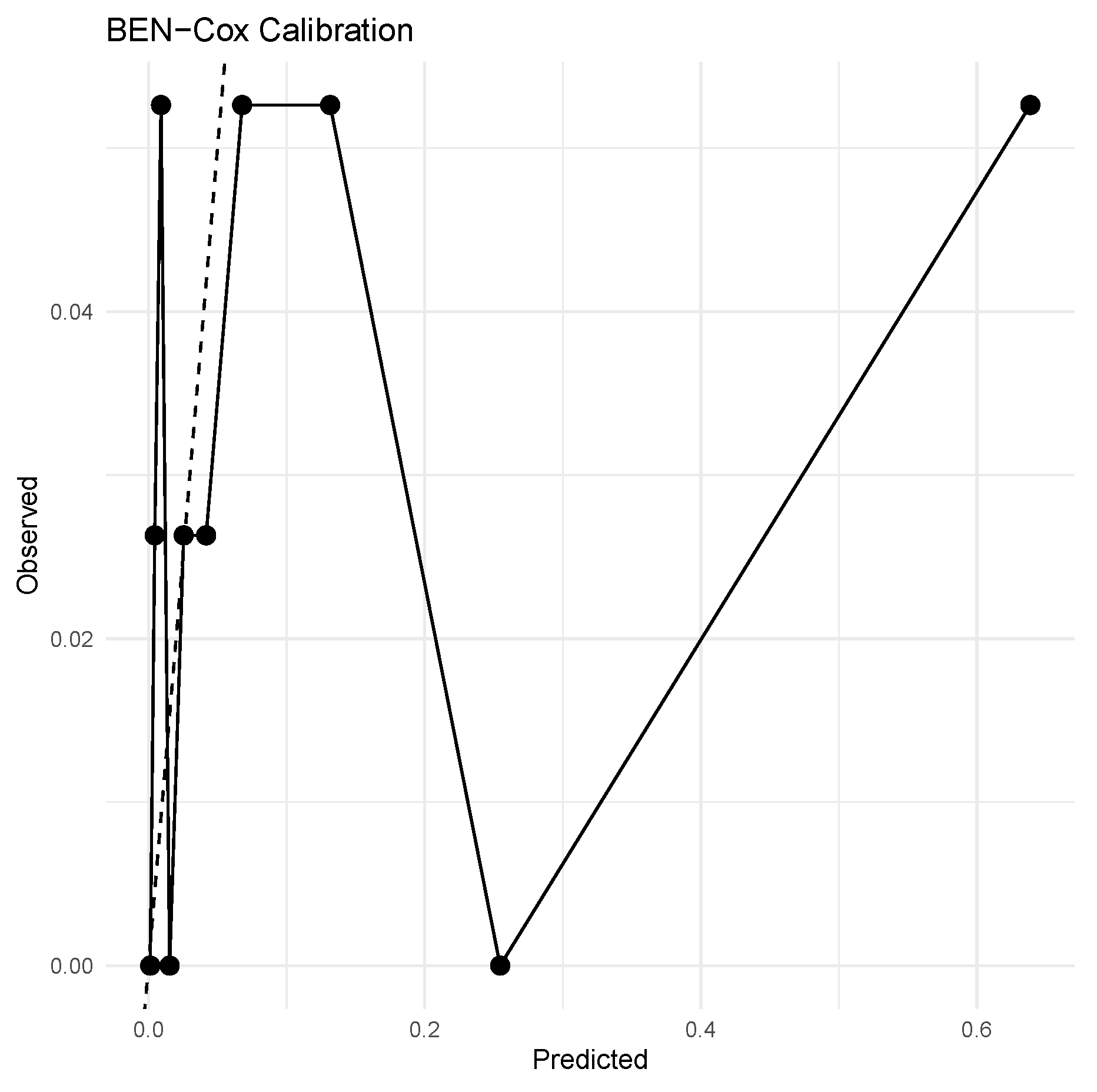
Figure 5.
Posterior means and 95% credible intervals for the 30 largest BEN–Cox regression coefficients. The selected panel is sparse (48 genes overall) and includes ERBB2 from the PAM50 signature.
Figure 5.
Posterior means and 95% credible intervals for the 30 largest BEN–Cox regression coefficients. The selected panel is sparse (48 genes overall) and includes ERBB2 from the PAM50 signature.
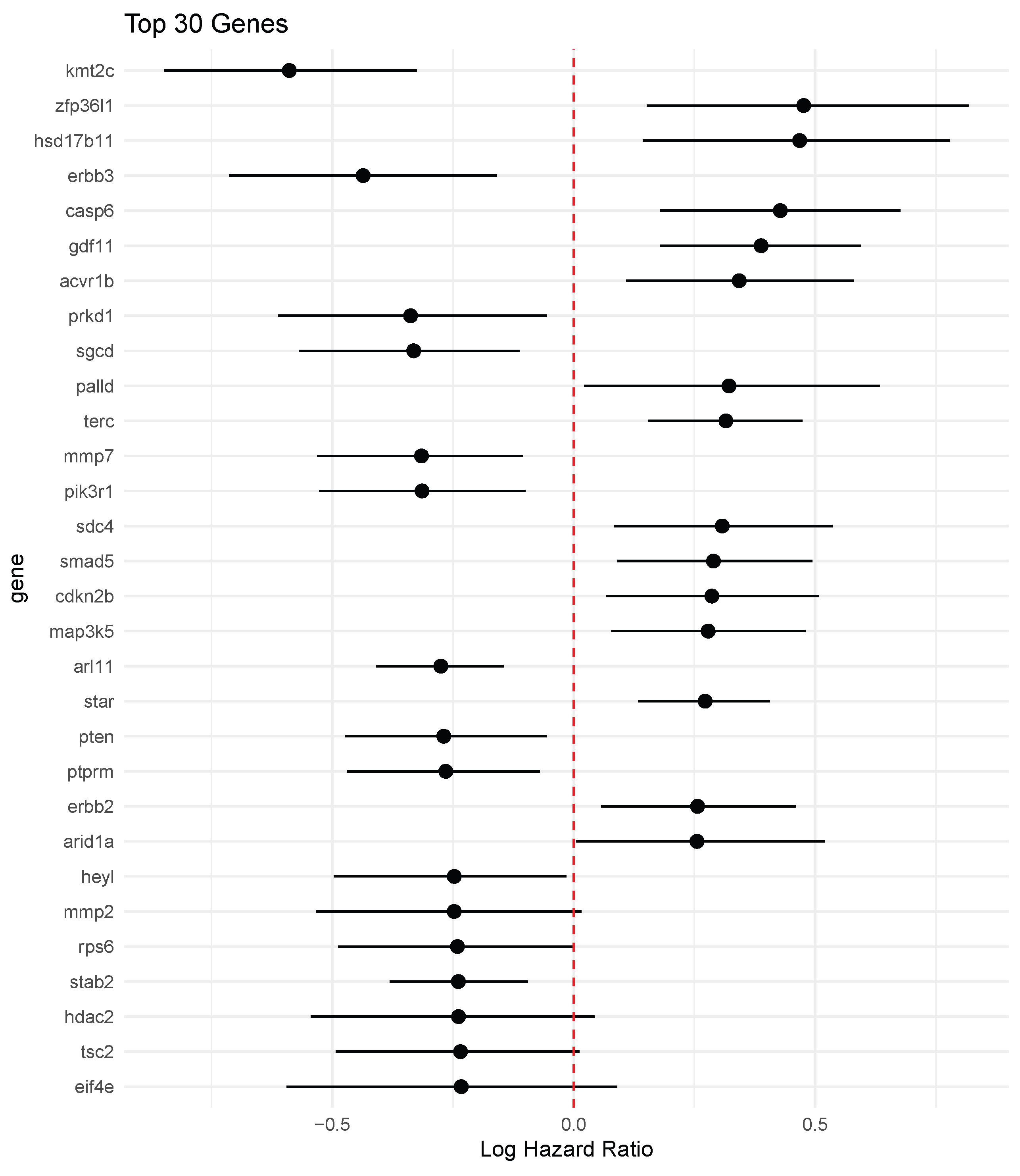
Table 4 summarizes coverage of the PAM50 gene panel for the ridge and BEN–Cox models. The ridge Cox model, which retains all 440 pre-filtered features with non-zero coefficients, effectively achieves full recall of the PAM50 genes present in the expression matrix. In contrast, BEN–Cox retains 48 genes in total and recovers about one third of the PAM50 genes available in this reduced panel (33.3% recall). This behaviour is consistent with the design of the elastic–net prior: it aggressively shrinks weak or redundant signals, aiming to identify a compact subset of strongly prognostic genes rather than reproduce the full PAM50 signature.
In summary, the BEN–Cox model on METABRIC satisfies standard convergence diagnostics, yields a sparse and interpretable panel of 48 prognostic genes, and achieves *slightly better* discrimination and prediction error on the held-out test set than a tuned ridge-penalised Cox model. Both penalised models substantially outperform the null Cox model in terms of discrimination, but BEN–Cox attains a smaller IBS and a higher C-index than ridge, with differences that are small but consistent across bootstrap resamples.
From a calibration perspective, the GND statistic indicates that BEN–Cox has a moderate lack of fit, whereas the ridge model shows a much larger global miscalibration signal. Taken together, these results suggest that BEN–Cox offers a more favourable trade-off: it delivers marginally better discrimination and lower prediction error than ridge while also exhibiting substantially better calibration and a much more compact gene signature. The fact that the selected panel still recovers ERBB2 from the PAM50 panel aligns with known biology and supports the interpretability of the learned effects.
These findings support the idea that a fully Bayesian elastic–net prior can deliver a sparse, biologically plausible high-dimensional survival model that slightly improves upon ridge in discrimination, prediction error, and calibration, while offering full posterior uncertainty quantification for hazard ratios and survival curves.
5. Discussion
The Bayesian elastic–net Cox model achieved discrimination on METABRIC that is slightly better than a tuned ridge-penalized Cox baseline, while producing a substantially sparser set of prognostic genes and providing coherent posterior uncertainty estimates. At the same time, the BEN–Cox model showed more favourable calibration according to the GND statistic, suggesting that a carefully constructed global–local prior can improve both discrimination and global fit relative to a purely -penalized approach. The grouping result in Theorem 1 helps explain the consistent retention of correlated gene-level feature clusters, in line with known gene modules and signatures such as ERBB2-related pathways.
Beyond the empirical METABRIC analysis, the methodological contribution is the theoretical support for BEN–Cox in the high-dimensional Cox setting. Especially, Theorem 1 formalizes a Bayesian analogue of the elastic-net grouping effect at the posterior mode, which is practically important in gene-expression studies because strongly correlated genes in the dataset tend to move together and form biologically meaningful modules. Moreover, Theorem 2 establishes posterior contraction under sparsity for the Cox partial-likelihood geometry (with a ridge component ensuring stability), which provides reassurance that the inferred risk score and the associated uncertainty quantification are statistically well-behaved as n grows. In this sense, the paper is not only an applied Bayesian survival analysis, but also a theoretical shrinkage construction specialized to the Cox partial-likelihood framework.
Limitations of the current study include computational cost (HMC is more expensive than deterministic optimisation), and the fact that all results are derived from a single cohort. External validation on independent datasets, and extensions to multi-cohort or hierarchical BEN–Cox formulations, would provide a stronger assessment of transportability. Another limitation is that we focused solely on gene-expression features; integrating clinical covariates and mutation data may further improve both calibration and interpretability.
Regarding the assumption justification of the introduced estimator in this specific METABRIC data analysis, by considering (A1–A5), we can infer the following: Our pre-processing enforces (A1) by z-scoring each feature on the training split and carrying scalings to the test set, which also bounds design entries after low-variance filtering. Regarding (A2), overall-survival times are observed on a finite horizon and the Cox partial likelihood is smooth; Breslow’s baseline estimator is standard in this setting [19]. For (A3), the compatibility/restricted-eigenvalue condition is plausible after variance filtering and with the stabiliser in the prior; empirically, the observed partial-likelihood information has well-behaved restricted spectra on supports of the selected size. The sparsity/growth condition (A4) is consistent with our use of elastic–net shrinkage to target a low-to-moderate number of effective gene features relative to n. Finally, (A5) holds by construction: half–Cauchy hyperpriors put sufficient mass near the canonical scale while keeping with high probability [18]. Overall, these checks support the applicability of the theoretical guarantees to the METABRIC data analysis.
Future work will explore multi-study hierarchical BEN models, integration of additional omics layers (e.g. somatic mutation data), and explicit calibration-improving extensions, for example, by combining BEN–Cox with Bayesian isotonic regression or flexible baseline hazard modelling.
6. Conclusion
In this study, we introduced a fully Bayesian elastic–net Cox (BEN–Cox) model for high-dimensional time–to–event analysis and applied it to the METABRIC breast cancer cohort using only gene–expression features. The model combines an elastic–net type prior with HMC to produce sparse coefficient estimates together with full posterior uncertainty for hazard ratios and survival curves. A fully Bayesian elastic–net Cox model offers an interpretable and sparse risk score using only gene–expression features from the METABRIC dataset. On this moderate level high–dimensional dataset, with 440 gene–level predictors after quality control, the BEN–Cox model achieves slightly lower integrated Brier score, slightly higher C–index, and a clearly smaller GND statistic than a tuned ridge–penalised Cox model on the held–out test set (Table 3). In other words, within this setting BEN–Cox provides a modest but consistent improvement in prediction error, discrimination, and global calibration while still yielding a compact number of genes and full posterior uncertainty quantification.
The main conclusions of this study can be summarized as follows:
- BEN–Cox selects a small set of prognostic genes (48 in our analysis), with posterior credible intervals that help quantify the strength and direction of each effect, and it recovers biologically meaningful markers such as ERBB2.
- In terms of predictive performance, compared with a tuned ridge Cox model, BEN–Cox shows slightly better integrated Brier score, slightly higher C–index, and noticeably better global calibration as measured by the GND statistic, while both models clearly outperform the null Cox baseline.
- The Stan HMC implementation delivers full posterior distributions for regression coefficients and survival curves, offering coherent uncertainty quantification at both the gene and patient level.
- Despite the Bayesian formulation and MCMC, the complete pipeline (fitting, bootstrap evaluation, and plotting) remains computationally feasible on standard hardware for a cohort of this size.
- Here it can be said that the introduced theoretical results emphasize the theoretical contribution of the paper which is the Bayesian grouping property explains stable behavior under strong gene correlations, and the posterior contraction result provides an asymptotic guarantee that the BEN–Cox posterior concentrates around sparse truth at the usual high-dimensional rate in the Cox partial-likelihood setting.
At the same time, the remaining imperfections in calibration and the reliance on a single cohort highlight the need for future work on Bayesian calibration strategies, multi–cohort or hierarchical extensions of BEN–Cox, and integration of additional clinical and molecular covariates in high–dimensional time–to–event prediction.
Author Contributions
Conceptualization: E.Y., S.E.A. & D.A.; Methodology: E.Y. & S.E.A.; Software and coding: E.Y. Formal analysis and investigation: E.Y.; Data curation: E.Y.; Supervision: S.E.A. & D.A.; Writing – original draft: E.Y.; D.A. Writing – review & editing: S.E.A., D.A. & E.Y.
Funding
Not applicable.
Data Availability Statement
Gene-expression and clinical data from the METABRIC breast-cancer cohort are publicly available through cBioPortal (Breast Invasive Carcinoma (METABRIC), Nature 2012 & Nat Commun 2016; see https://www.cbioportal.org/study/summary?id=brca_metabric).
Acknowledgments
The research of Professor S. Ejaz Ahmed was supported by the Natural Sciences and the Engineering Research Council (NSERC) of Canada.
Conflicts of Interest
The authors do not have any conflict of interest.
Code availability
R and Stan code implementing the BEN–Cox model and reproducing the analyses in this article are available at https://github.com/yilmazersin13/Bayesian-Elastic-Net-Cox-Model-.
Appendix A. Proof of Theorem 2
We give a concise contraction proof in the standard Bayesian form (tests + prior mass + complexity), adapted to the Cox partial-likelihood setting; see Ghosal and van der Vaart [13] for the general contraction theory. Let be the true -sparse vector with support , and define .
We can consider the partial likelihood ratio as follows: By Lemma 1 and (A2), is twice continuously differentiable and concave. Therefore, a Taylor expansion around yields, for in a neighbourhood of ,
for some on the line segment between and , where is the observed partial-likelihood information.
Under the Cox model, is a score term with mean zero, and the restricted curvature condition (A3) implies that on sparse directions (support size ), locally around . Hence, on sparse neighbourhoods, the likelihood separates quadratically at rate , up to the usual stochastic score fluctuations.
Define the alternative set Using the local quadratic separation implied by (A3) together with the non-iid testing construction in Ghosal and van der Vaart [13], there exist tests and constants such that, for large n and M sufficiently large,
This provides exponentially powerful tests at the target scale.
We now lower bound the prior mass assigned to an -ball around . Consider
By Lemma 2, the marginal prior under fixed is proportional to Take and ; by (A5) the half-Cauchy hyperpriors assign positive mass to such a region. Conditional on such , the prior density is continuous and bounded away from zero in a small neighbourhood of , hence
Therefore, after integrating over using (A5), we obtain
for some constant .
Finally, we control the complexity of the effective parameter space. Let for a fixed large R. Standard sparse covering arguments yield
Combining the existence of exponentially consistent tests, the prior mass bound , and the entropy bound , the general posterior contraction theorem for non-iid observations in Ghosal and van der Vaart [13] gives that there exists such that
This proves Theorem 2.
References
- Cox, D.R. Regression models and life-tables. Journal of the Royal Statistical Society: Series B (Statistical Methodology) 1972, 34, 187–220. [Google Scholar] [CrossRef]
- Zou, H.; Hastie, T. Regularization and variable selection via the elastic net. Journal of the Royal Statistical Society: Series B (Statistical Methodology) 2005, 67, 301–320. [Google Scholar] [CrossRef]
- Simon, N.; Friedman, J.; Hastie, T.; Tibshirani, R. Regularization paths for Cox’s proportional hazards model via coordinate descent. Journal of Statistical Software 2011, 39, 1–13. [Google Scholar] [CrossRef] [PubMed]
- Witten, D.M.; Tibshirani, R. Survival analysis with high-dimensional covariates. Statistical Methods in Medical Research 2010, 19, 29–51. [Google Scholar] [CrossRef] [PubMed]
- Ahmed, S.E.; Arabi Belaghi, R.; Hussein, A.A. Efficient post-shrinkage estimation strategies in high-dimensional Cox’s proportional hazards models. Entropy 2025, 27, 254. [Google Scholar] [CrossRef] [PubMed]
- Gao, X.; Ahmed, S.E.; Feng, Y. Post-selection shrinkage estimation for high-dimensional data analysis. Applied Stochastic Models in Business and Industry 2017, 33, 97–120. [Google Scholar] [CrossRef]
- Hossain, S.; Ahmed, S.E. Penalized and shrinkage estimation in the Cox proportional hazards model. Communications in Statistics - Theory and Methods 2014, 43, 1026–1040. [Google Scholar] [CrossRef]
- Ahmed, S.E.; Hossain, S.; Doksum, K.A. LASSO and shrinkage estimation in Weibull censored regression models. Journal of Statistical Planning and Inference 2012, 142, 1273–1284. [Google Scholar] [CrossRef]
- Ahmed, S.E.; Ahmed, F.; Yüzbaşı, B. Post-shrinkage strategies in statistical and machine learning for high dimensional data; Chapman & Hall/CRC, 2023. [Google Scholar]
- Park, T.; Casella, G. The Bayesian lasso. Journal of the American Statistical Association 2008, 103, 681–686. [Google Scholar] [CrossRef]
- Li, Q.; Lin, N. The Bayesian elastic net. Bayesian Analysis 2010, 5, 151–170. [Google Scholar] [CrossRef]
- Hans, C. Elastic net regression modelling with the orthant normal prior. Journal of the American Statistical Association 2011, 106, 1383–1393. [Google Scholar] [CrossRef]
- Ghosal, S.; van der Vaart, A.W. Convergence rates of posterior distributions for non-iid observations. The Annals of Statistics 2007, 35, 192–223. [Google Scholar] [CrossRef]
- Curtis, C.; Shah, S.P.; Chin, S.F.; Turashvili, G.; Rueda, O.M.; Dunning, M.J.; et al. The genomic and transcriptomic architecture of 2,000 breast tumours reveals novel subgroups. Nature 2012, 486, 346–352. [Google Scholar] [CrossRef]
- Demler, O.V.; Paynter, N.P.; Cook, N.R. Tests of calibration and goodness-of-fit in the survival setting. Statistics in Medicine 2015, 34, 1659–1680. [Google Scholar] [CrossRef]
- Hoffman, M.D.; Gelman, A. The no-u-turn sampler: adaptively setting path lengths in Hamiltonian Monte Carlo. Journal of Machine Learning Research 2014, 15, 1593–1623. [Google Scholar]
- Betancourt, M. A conceptual introduction to Hamiltonian Monte Carlo. arXiv 2017, arXiv:1701.02434. [Google Scholar]
- Gelman, A. Prior distributions for variance parameters in hierarchical models. Bayesian Analysis 2006, 1, 515–533. [Google Scholar] [CrossRef]
- Breslow, N.E. Covariance analysis of censored survival data. Biometrics 1974, 30, 89–99. [Google Scholar] [CrossRef] [PubMed]
- Pereira, B.; Chin, S.F.; Rueda, O.M.; et al. The somatic mutation profiles of 2,433 breast cancers refine their genomic and transcriptomic landscapes. Nature Communications 2016, 7, 11479. [Google Scholar] [CrossRef] [PubMed]
- Cerami, E.; Gao, J.; Dogrusoz, U.; et al. The cBio cancer genomics portal: an open platform for exploring multidimensional cancer genomics data. Cancer Discovery 2012, 2, 401–404. [Google Scholar] [CrossRef] [PubMed]
Figure 1.
Probabilistic graphical model for the Bayesian Elastic Net Cox (BEN-Cox) regression framework showing the hierarchical prior structure and survival data likelihood. The model employs a normal-exponential mixture representation of the elastic net prior as specified in equations (3)-(5). Shaded nodes represent observed variables while unshaded nodes denote latent variables and parameters. Rectangular plates indicate replication over feature (j) and subject (i) indices.
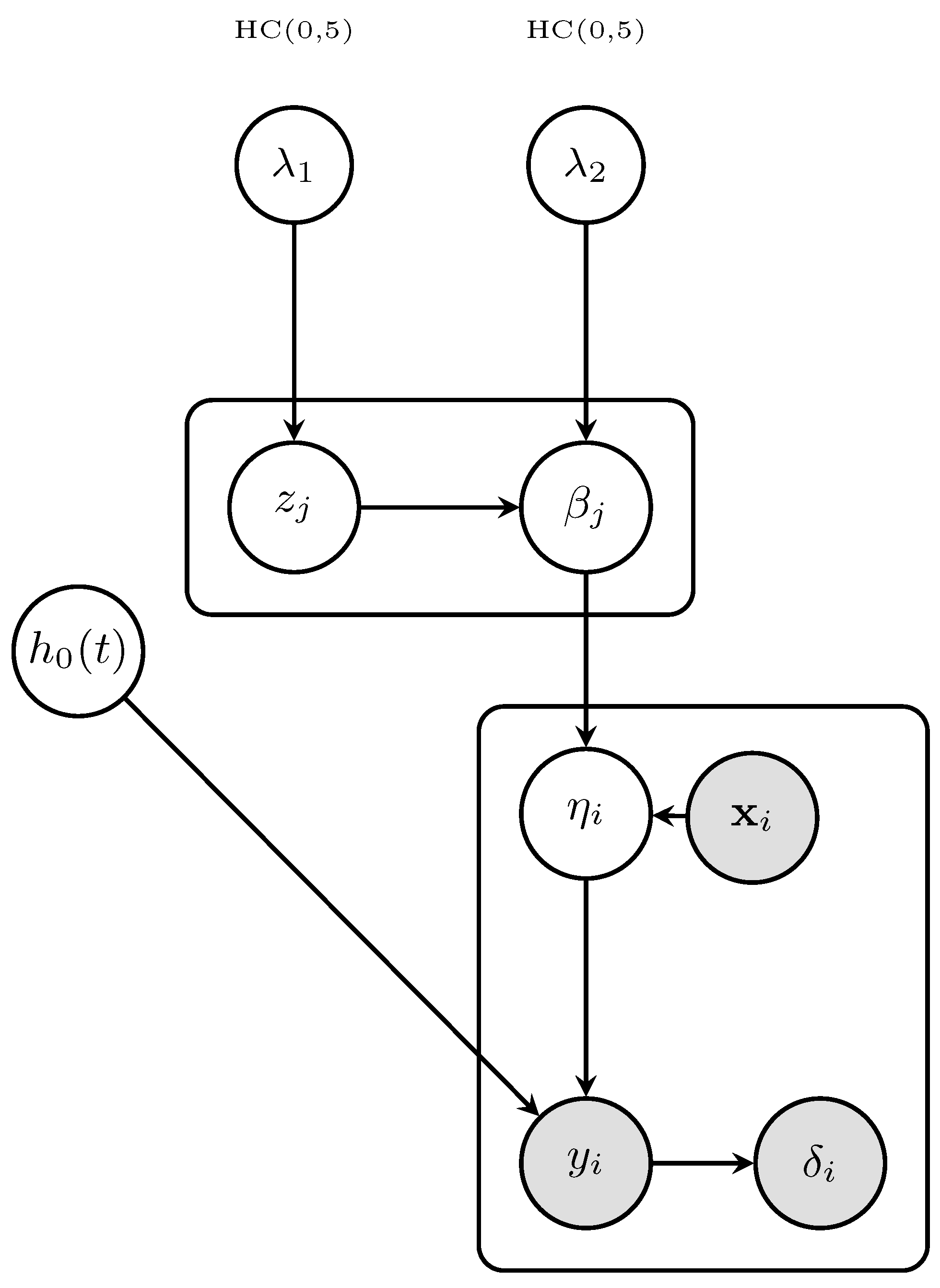
Figure 2.
Representative MCMC trace plots for the BEN–Cox model: global shrinkage parameters and selected regression coefficients across HMC iterations. The traces show good mixing and no systematic drift, in line with the and ESS values in Table 2.
Figure 2.
Representative MCMC trace plots for the BEN–Cox model: global shrinkage parameters and selected regression coefficients across HMC iterations. The traces show good mixing and no systematic drift, in line with the and ESS values in Table 2.
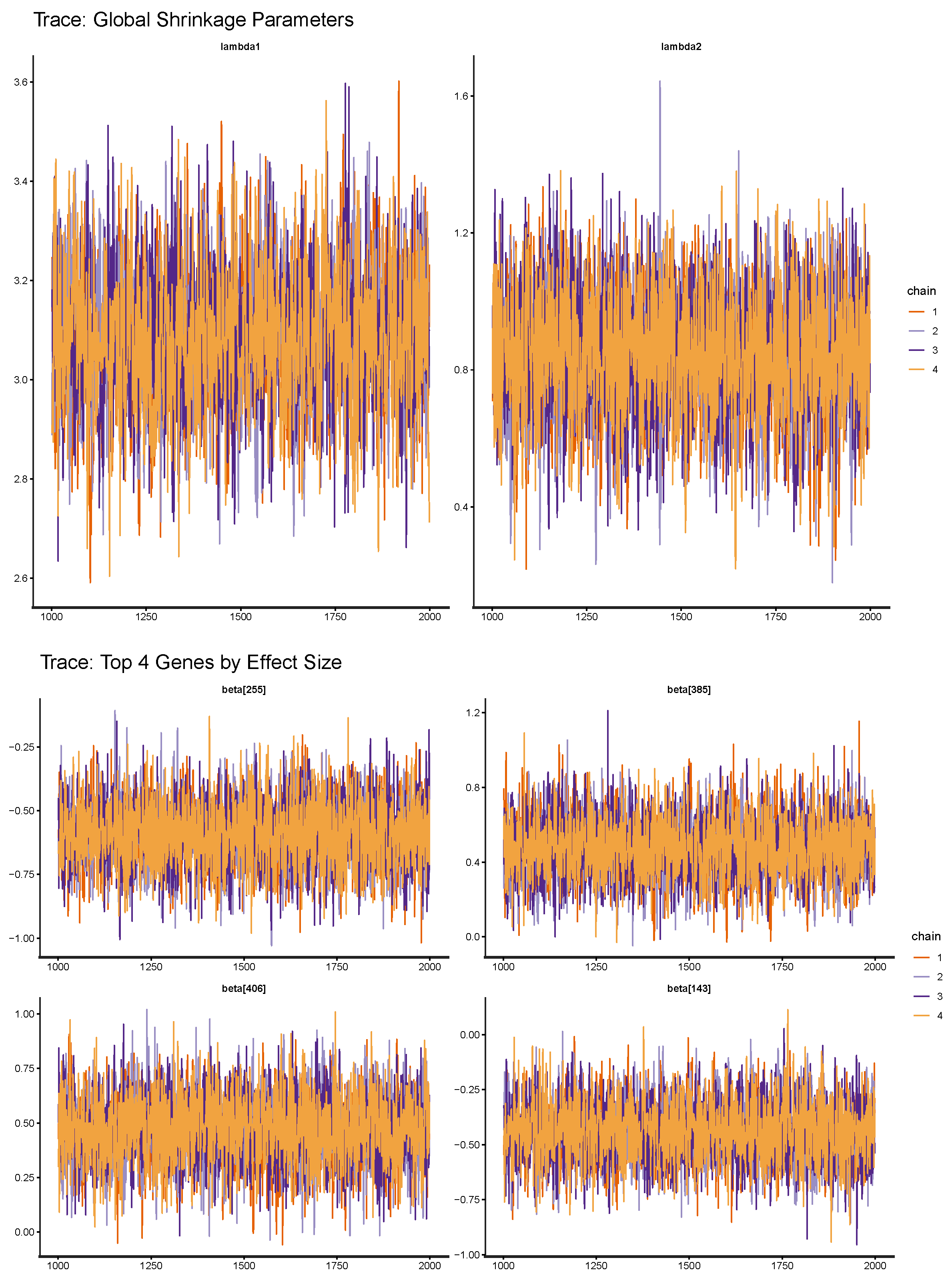
Figure 3.
Kaplan–Meier curves on the test set by quintiles of the BEN–Cox risk score. Higher-risk quintiles show worse survival, indicating that the model’s risk score meaningfully stratifies patients.
Figure 3.
Kaplan–Meier curves on the test set by quintiles of the BEN–Cox risk score. Higher-risk quintiles show worse survival, indicating that the model’s risk score meaningfully stratifies patients.
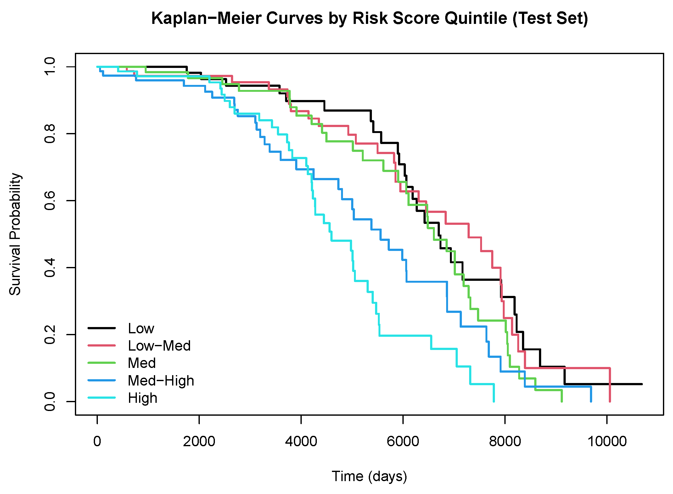

Table 1.
Summary of the METABRIC dataset after quality control.
| Quantity | Value |
|---|---|
| Number of patients (after QC) | 1903 |
| Number of events (deaths) | 800 (42.0%) |
| Median follow-up (years) | 16.4 |
| Gene-level features before filtering | 489 |
| Gene-level features after 10% variance filter | 440 |
| Training set size | 1522 subjects |
| Test set size | 381 subjects |
Table 2.
Convergence diagnostics for the Stan BEN–Cox fit on the training set. is the split- statistic across chains; ESS denotes the effective sample size.
Table 2.
Convergence diagnostics for the Stan BEN–Cox fit on the training set. is the split- statistic across chains; ESS denotes the effective sample size.
| Parameter | ESS | |
|---|---|---|
| Beta (median over coefficients) | 0.9997 | 4714 |
| Lambda1 | 1.0006 | 2288 |
| Lambda2 | 1.0008 | 4431 |
Table 3.
Predictive performance on the held-out 20% test set. Values are mean ± standard error over 100 bootstrap resamples. Lower IBS and GND indicate better prediction error and calibration, respectively; higher C-index indicates better discrimination.
Table 3.
Predictive performance on the held-out 20% test set. Values are mean ± standard error over 100 bootstrap resamples. Lower IBS and GND indicate better prediction error and calibration, respectively; higher C-index indicates better discrimination.
| Model | IBS ↓ | C-index ↑ | GND ↓ |
|---|---|---|---|
| Null Cox | 0.222 ± 0.014 | 0.500 ± 0.000 | 04.5 ± 1.0 |
| Ridge Cox | 0.224 ± 0.013 | 0.647 ± 0.026 | 89.4 ± 38.8 |
| BEN Cox | 0.216 ± 0.013 | 0.655 ± 0.027 | 18.9 ± 4.1 |
Table 4.
Coverage of the PAM50 gene panel among retained coefficients. For BEN Cox, “Genes retained” counts coefficients whose 95% posterior credible interval excludes zero.
Table 4.
Coverage of the PAM50 gene panel among retained coefficients. For BEN Cox, “Genes retained” counts coefficients whose 95% posterior credible interval excludes zero.
| Model | Genes retained | Recall (%) |
|---|---|---|
| Ridge Cox | 440 | 100.0 |
| BEN Cox | 48 | 33.3 |
Disclaimer/Publisher’s Note: The statements, opinions and data contained in all publications are solely those of the individual author(s) and contributor(s) and not of MDPI and/or the editor(s). MDPI and/or the editor(s) disclaim responsibility for any injury to people or property resulting from any ideas, methods, instructions or products referred to in the content. |
© 2026 by the authors. Licensee MDPI, Basel, Switzerland. This article is an open access article distributed under the terms and conditions of the Creative Commons Attribution (CC BY) license (http://creativecommons.org/licenses/by/4.0/).
Copyright: This open access article is published under a Creative Commons CC BY 4.0 license, which permit the free download, distribution, and reuse, provided that the author and preprint are cited in any reuse.


