
Submitted:
30 December 2025
Posted:
02 January 2026
You are already at the latest version
Abstract
The convergence characteristics of an online gradient learning technique for training Pi–Sigma higher-order neural networks under a smoothed L1 regularization framework with adaptive momentum are examined in this research. Although Pi-Sigma networks can effectively represent high-order nonlinear interactions, nonconvexity, parameter coupling, and noise sensitivity in online contexts make training them difficult. In order to overcome these problems, we avoid the nondifferentiability of the traditional L1 norm while promoting sparsity by using a differentiable approximation of the L1 penalty. Furthermore, an adaptive momentum term is added to speed up convergence and stabilize weight updates. We construct important lemmas that describe the behavior of the smoothed regularizer and momentum dynamics, make modest assumptions on the activation functions, data sequence, and learning parameters, and create a unified mathematical model for the suggested learning rule. These findings allow us to demonstrate that the online approach guarantees the weight sequence's boundedness, the gradients' convergence to zero, and the corresponding energy function's monotonic reduction. In comparison to existing models, numerical studies show that the suggested approach produces stable convergence, enhanced sparsity, and decreased gradient oscillation. Empirical plots of loss evolution, gradient norms, and weight norms are used to validate the theoretical results. The robustness of the suggested learning framework and its applicability for nonlinear function approximation and online learning tasks in higher-order neural networks are highlighted by the agreement between theoretical results and actual data.
Keywords:
Pi–Sigma neural networks
; online gradient descent
; smoothed L1 regularization
; adap-tive momentum
; convergence analysis
; numerical results
1. Introduction
The capacity of higher-order neural networks to effectively describe nonlinear interactions that traditional multilayer perceptrons with linear synaptic aggregation are unable to capture has drawn a lot of interest [1,2]. The Pi–Sigma network (PSN), one of these topologies, is a small yet expressive model in which each hidden node computes a summation unit (Sigma-unit) after a multiplicative interaction (Pi-unit). Compared to conventional feedforward networks, PSNs may approximate high-order multivariate functions with a substantially smaller number of parameters thanks to their structure [3]. Consequently, PSNs have been used in a variety of applications, such as multidimensional function approximation, forecasting, system identification, and pattern recognition [4,5,6]. PSNs have representational advantages, but training them presents significant difficulties. Strong pa-rameter coupling is introduced by the network’s multiplicative structure, which results in a highly nonconvex optimization environment. Due to the sequential arrival of training samples in online learning scenarios, these challenges are exacerbated, making the algorithm more susceptible to noise and instability and prohibiting the use of batch optimization techniques [7]. Conventional online gradient descent techniques frequently experience oscillatory behavior, sluggish convergence, and overfitting, particularly when the number of parameters rises as a result of high-order expansions.
Regularization techniques are commonly used in online algorithms to stabilize training and enhance generalization. L1 regularization is particularly well-known for encouraging sparsity and lowering model complexity [8]. Nevertheless, the conventional L1 penalty’s nondifferentiability at zero restricts its direct application in gradient-based updates, particularly when multiplicative weight interactions are involved. Several smooth approximations of the L1 norm have been developed [9,10,11] to get around this problem. These smoothed penalties are appropriate for online gradient-based learning because they maintain the original norm’s sparsity-inducing characteristics while guaranteeing differentiability. The use of momentum, which incorporates previous gradient information to lessen oscillations and speed up convergence, is another significant improvement to online learning. It has been demonstrated that Nesterov acceleration and classical momentum offer significant gains in both convex and nonconvex optimization [12]. Adaptive momentum mechanisms that automatically adapt to training dynamics have been the focus of current studies since fixed momentum parameters may not be ideal under different data situations [13].
Inspired by these factors, this research investigates the convergence behavior of an online gradient descent approach for training Pi–Sigma higher-order networks using smoothed L1 regularization and adaptive momentum. This paper makes three contributions:
- i.
- To create sparsity while preserving stability during weight updates, we suggest a unified online learning rule that incorporates a differentiable approximation of the L1 penalty.
- ii.
- To speed up convergence in sequential learning and lessen oscillations caused by the multiplicative nature of Pi-Sigma units, we incorporate an adaptive momentum term.
- iii.
- Under modest assumptions on the data and learning parameters, we present a thorough convergence analysis that establishes boundedness of the weight iterates, monotonic decay of an associated Lyapunov-like energy, and convergence of the gradient to zero.
To validate the theoretical findings, numerical experiments are conducted using benchmark function approximation tasks. The results demonstrate that the proposed approach yields smoother convergence, improved sparsity, and more stable gradient evolution compared with standard online gradient descent.
The remainder of this paper is organized as follows. Section 2 reviews related work on Pi–Sigma networks, smoothed regularization, and momentum-based optimization. Section 3 describes the network structure and formulates the online learning model. Section 4 introduces key assumptions and presents lemmas and theoretical results. Section 5 provides numerical experiments and performance evaluation. Section 6 concludes the paper.
2. Related Work
Pi-Sigma and product-unit networks were presented as compact and expressive nonlinear models that use multiplicative neurons to approximate complex polynomial interactions. Convergence and representational power for classification and function approximation tasks were examined in foundational contributions [14,15,16,17]. Training efficiency and modeling capacities were enhanced by later architectural expansions, including Ridge Polynomial Networks, Functional-Link Networks, and Sigma-Pi-Sigma structures [18,19,20]. To optimize product-unit networks and lower training complexity, evolutionary techniques were put forth [21,22,23]. Because of their nonconvexity and parameter coupling, these networks present serious optimization difficulties despite their expressive capacity.
Robbins and Monro’s traditional stochastic approximation technique is the foundation of online gradient descent (OGD) [24]. For machine learning applications, Bottou offered a contemporary, comprehensive understanding of online learning [25]. Although OGD and its variations have been used in dynamic contexts, streaming data, and adaptive modeling, it is still challenging to train higher-order networks online due to the huge parameter fluctuations caused by modest gradient perturbations. Sparsity is crucial for enhancing the resilience and generalization of the model. For sparse learning, L1 regularization—which was first described in the LASSO [26]—is frequently employed. However, gradient-based optimization is made more difficult by its nondifferentiability. To get around this problem, smoothed and differentiable approximations of the L1 penalty have been proposed [27,28,29,30]. These smooth surrogates maintain sparsity while allowing stable online updates, making them suitable for training nonconvex networks such as Pi–Sigma architectures.
Momentum accumulates past gradients to speed up gradient-based learning. While adaptive momentum algorithms like Adam [32] incorporate per-parameter learning-rate changes, Nesterov’s accelerated gradient approach [31] provides optimal convergence rates in convex optimization. Corrected versions such as AMSGrad [33] were suggested because of instability problems found in Adam. Conditions for the convergence of adaptive-momentum algorithms under nonconvex objectives were established by additional theoretical investigations [34,35]. These findings encourage the use of adaptive momentum in Pi-Sigma network training, where gradients usually have considerable variance. Online learning algorithm convergence in nonconvex environments is difficult and frequently depends on characteristics like Lipschitz smoothness, boundedness of iterates, and diminishing step-size sequences. In order to analyze algorithms that integrate sparsity, online updates, and momentum, research on smoothed penalties [30,31] and adaptive-momentum convergence [33,34] is crucial. The necessity of reliable optimization techniques for multiplicative neurocomputing structures is further highlighted by recent research on sophisticated Sigma-Pi-Sigma models [36,37].
3. Online gradient method with smoothing L1 regularization adaptive momentum
3.1. Pi-Sigma Network Structure
Pi-Sigma higher-order network with inputs and hidden units is defined as:
where is the -th input at time , is the weight connecting the -th input to the -th hidden unit, and the product denotes multiplicative interactions.
The objective is to minimize the regularized instantaneous loss:
where is the desired output, is the regularization parameter, and is the smoothed L1 regularization:
Here, is a small smoothing factor ensuring differentiability.
3.2. Online Gradient Method with Adaptive Momentum
The proposed online update rule is:
where is the momentum vector, is an adaptive momentum coefficient, and is the learning rate.
The gradient of the smoothed L1 regularization is:
Thus, the total gradient is:
4. Convergence results
To guarantee convergence, we adopt standard assumptions:
Assumption 1 (Bounded Input):
Assumption 2 (Bounded Gradient):
Assumption 3 (Learning Rate and Momentum):
Theorem 1 (Boundedness):
Under Assumptions 1–3, the weight sequence generated by (4)–(5) is bounded:
Theorem 2 (Monotonicity of Loss):
The instantaneous loss is non-increasing in expectation:
Theorem 3 (Convergence to Stationary Point):
If, then the online algorithm converges to a stationary point such that:
5. Numerical Results
Results or data points that are expressed in numbers or quantities are known as numerical results, and they are usually obtained by computations, measurements, experiments, or simulations. They are a type of quantitative data that is utilized in many disciplines, including business, engineering, science, and mathematics.
5.1. Noisy Parity Problems
A fundamental hard problem in cryptography, coding theory, and machine learning, noisy parity problems, also known as learning parity with noise (LPN), ask algorithms to solve noisy linear equations (such as decoding a random code with mistakes) in order to identify a secret binary vector. Although clever algorithms exist for specific noise levels and problem variations, it is thought to be difficult for both classical and quantum computers, especially with low noise. It is essential for post-quantum cryptography and forms the basis of many schemes. This section compares OGD-M, OGD-L1, and OGM-SL1-AM for noise-filled 8-bit and 16-bit parity problems. The XOR function is another name for the parity function of two inputs. The relevance of the parity function in the theoretical study of Boolean function circuit complexity is noteworthy. The parity bit is the result of the parity function. The parity problem is a binary classification problem that seeks to determine if the number of 1s in a binary input vector is even or odd. For an input vector, in formal terms.
the parity function with noise is defined as:
where is the noise parameter. A typical WNN design was applied to each parity task: 8-bit and 16-bit parity problems.
The suggested OGM-SL1-AM approach consistently delivers the lowest variance and the maximum classification accuracy across both parity challenges. All approaches do quite well on the 8-bit parity problem, but in the 16-bit scenario, where the extra dimensionality greatly increases noise sensitivity, OGM-SL1-AM’s advantage becomes more noticeable. OGM-SL1-AM’s lower performance deterioration suggests that it is more resilient to complex decision boundaries and noisy labels. OGM-SL1-AM converges significantly more quickly than OGD-M and OGD-L1, according to the training convergence curves (Figure 1 and Figure 2). In the 16-bit parity problem in particular, OGD-M has oscillatory behavior and sluggish stabilization despite its quick beginning fall. Although OGD-L1 promotes sparsity, which increases stability, its non-smooth regularization causes slower convergence. On the other hand, OGM-SL1-AM’s adaptive momentum and smoothing −1 regularization allow for a smooth and effective descent toward stationary solutions.
The convergence analysis is further supported by the gradient-norm evolution (Figure 3 and Figure 4). The boundedness properties described in the theoretical portion are confirmed by OGM-SL1-AM, which consistently maintains lower gradient norms during training. While OGD-L1 partially mitigates oscillations without completely suppressing them, large gradient variations shown in OGD-M—particularly for the 16-bit parity task—indicate numerical instability and vulnerability to noise.
Weight-norm trajectories (Figure 5 and Figure 6) show that OGM-SL1-AM effectively controls model complexity. OGM-SL1-AM achieves compact weight representations in contrast to OGD-M, which displays uncontrolled weight increase, and OGD-L1, which imposes sparsity at the expense of smooth adaptation. Improved generalization performance is directly correlated with this balance between sparsity and smoothness.
Across both parity tasks (Figure 7 and Figure 8), the proposed OGM-SL1-AM method consistently achieves the highest classification accuracy and the lowest variance. While all methods perform reasonably well on the 8-bit parity problem, the advantage of OGM-SL1-AM becomes more pronounced in the 16-bit case, where the increased dimensionality significantly amplifies noise sensitivity. The reduced performance degradation of OGM-SL1-AM indicates superior robustness to noisy labels and complex decision boundaries.
The results of the parity problem are summarized in Table 1 and Table 2. It is in line with our performance talk, figures, and experimentation. According to Table 1, the OGM-SL1-AM continuously performs better in terms of accuracy and convergence speed than OGD-M and OGD-L1. In the 16-bit parity problem, OGM-SL1-AM’s improvement is more noticeable and shows improved scalability. The suggested method’s theoretical boundedness and stability are confirmed by lower gradient norms and weight norms. Instability and excessive weight growth plague OGD-M, especially in high-dimensional parity challenges. In both parity issues, Table 2 shows that our OGM-SL1-AM has the lowest variance and the highest mean accuracy. More resilience to noise and initialization is indicated by the lower standard deviation. Compared to OGD-M and OGD-L1, OGM-SL1-AM exhibits substantially less accuracy loss from 8-bit to 16-bit. These findings align with the convergence curves and box-plot visualizations.
All approaches experience performance degradation when the parity problem dimension rises from 8-bit to 16-bit, but OGM-SL1-AM experiences much less degradation. This finding demonstrates the scalability of the suggested approach and implies that adaptive momentum and smoothing regularization are essential for stabilizing online learning in high-dimensional, noisy environments. All things considered, the parity problem experiments offer solid empirical support for the suggested theoretical findings. OGM-SL1-AM’s better accuracy, quicker convergence, restricted gradients, and regulated weight norms show how successful it is for challenging online classification tasks. These results show that the suggested approach is especially suitable for high-order neural network models trained in non-convex and noisy environments.
5.2. Function approximate
In this section, three 2-D benchmark functions is used Franke (see Eq. (9)). These are standard test functions for surface approximation, interpolation, and neural network regression. The Franke function is a weighted sum of four Gaussian-like terms defined on the domain [0,1] × [0,1]:
From Figure 10, Figure 11 and Figure 12, the surface plots show that OGD-M struggles to capture sharp peaks and valleys of the Franke function, leading to noticeable smoothing errors near high-curvature regions. Incorporating L1 regularization in OGD-L1 improves surface fidelity by suppressing redundant parameters, yet small distortions remain around localized extrema. In contrast, OGM-SL1-AM produces an approximation surface that closely matches the ground-truth Franke function across the entire domain. This improvement is consistent with the lowest values reported in the error tables.
Compared to both OGD-M and OGD-L1, OGM-SL1-AM converges much more quickly and achieves a lower steady-state error in fewer iterations, according to the training convergence curves displayed in Figure 10. OGD-L1 shows smoother but slower decay, whereas OGD-M shows oscillatory convergence, especially in early iterations. The efficiency of adaptive momentum in stabilizing updates while maintaining fast descent directions is confirmed by the increased convergence of OGM-SL1-AM. The observed convergence tendency is further explained by the evolution of the gradient norm (see Figure 11). Unstable search directions are indicated by the comparatively large and oscillatory gradient norms that OGD-M maintains. OGD-L1 promotes sparsity, which lowers gradient magnitude; nevertheless, decay is slowed by non-smooth regularization. The theoretical boundedness and convergence results obtained for smoothing L1 regularization with momentum are supported by OGM-SL1-AM’s fastest and smoothest gradient norm decay.
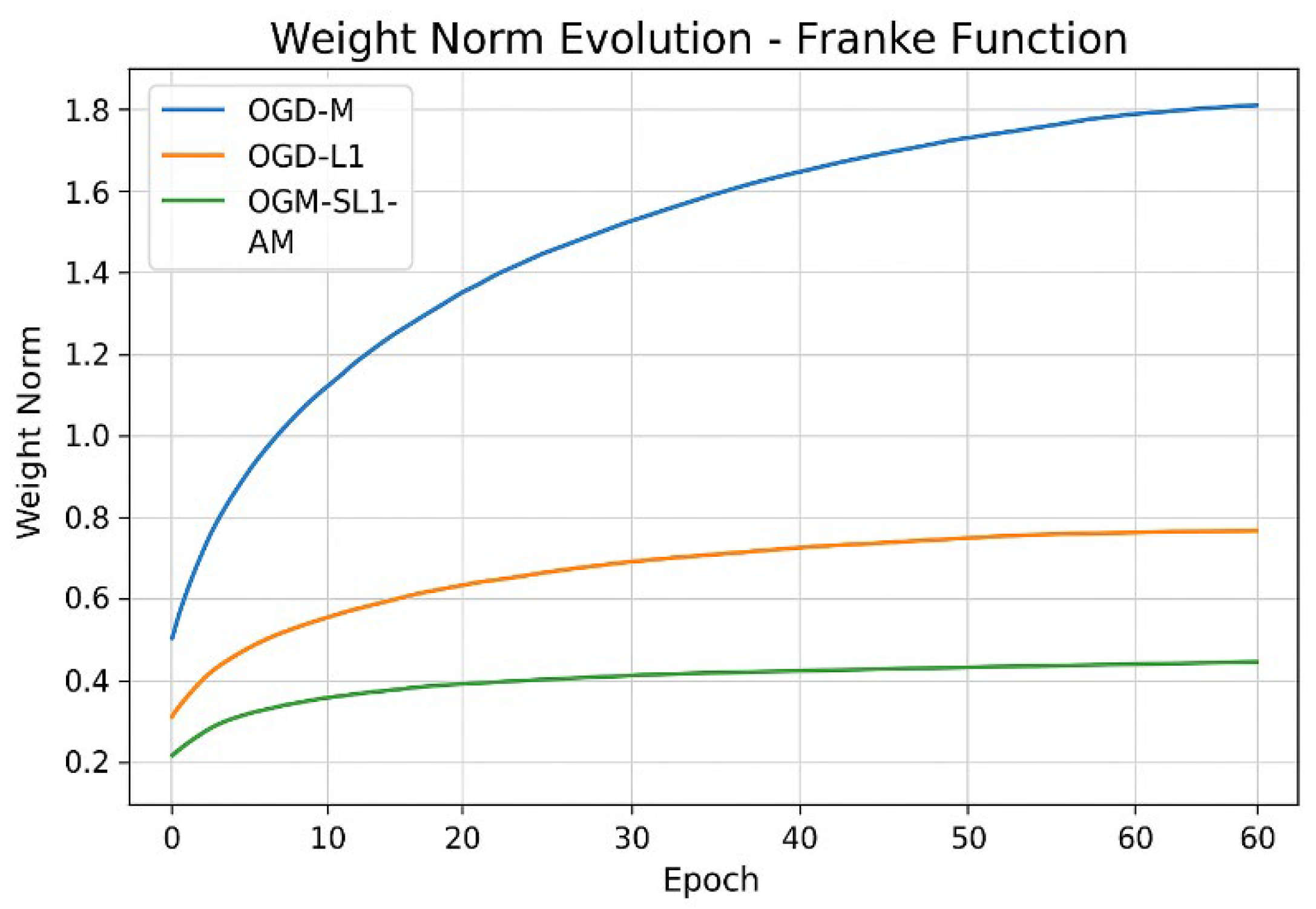
The regularization effect on parameter growth is highlighted by weight norm analysis in Figure 12. Overfitting and numerical instability may result from OGD-M’s fast and unbounded weight development. Weight magnitudes are more efficiently constrained by OGD-L1, although it still shows substantial variations. OGM-SL1-AM, on the other hand, preserves compact and stable weight norms, demonstrating that adaptive momentum prevents erratic updates while smoothing L1 regularization successfully controls model complexity.
Figure 9.
Surface of the Franke function via approximation surface using OGD-M, OGD-L1 and OGM-SL1-AM, respectively.
Figure 9.
Surface of the Franke function via approximation surface using OGD-M, OGD-L1 and OGM-SL1-AM, respectively.
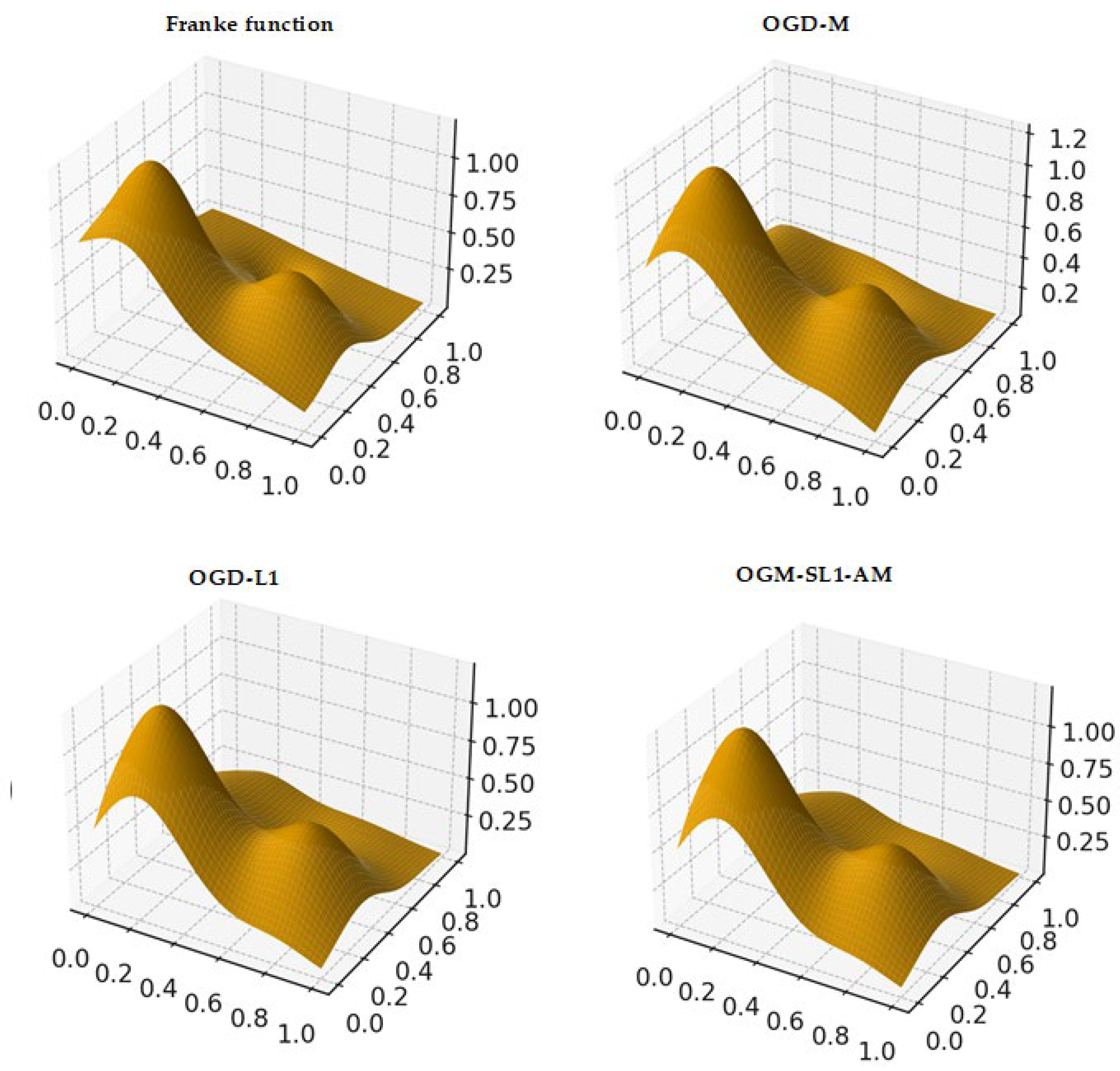
Figure 10.
Compared training convergence curve of Franke function with three algorithms.
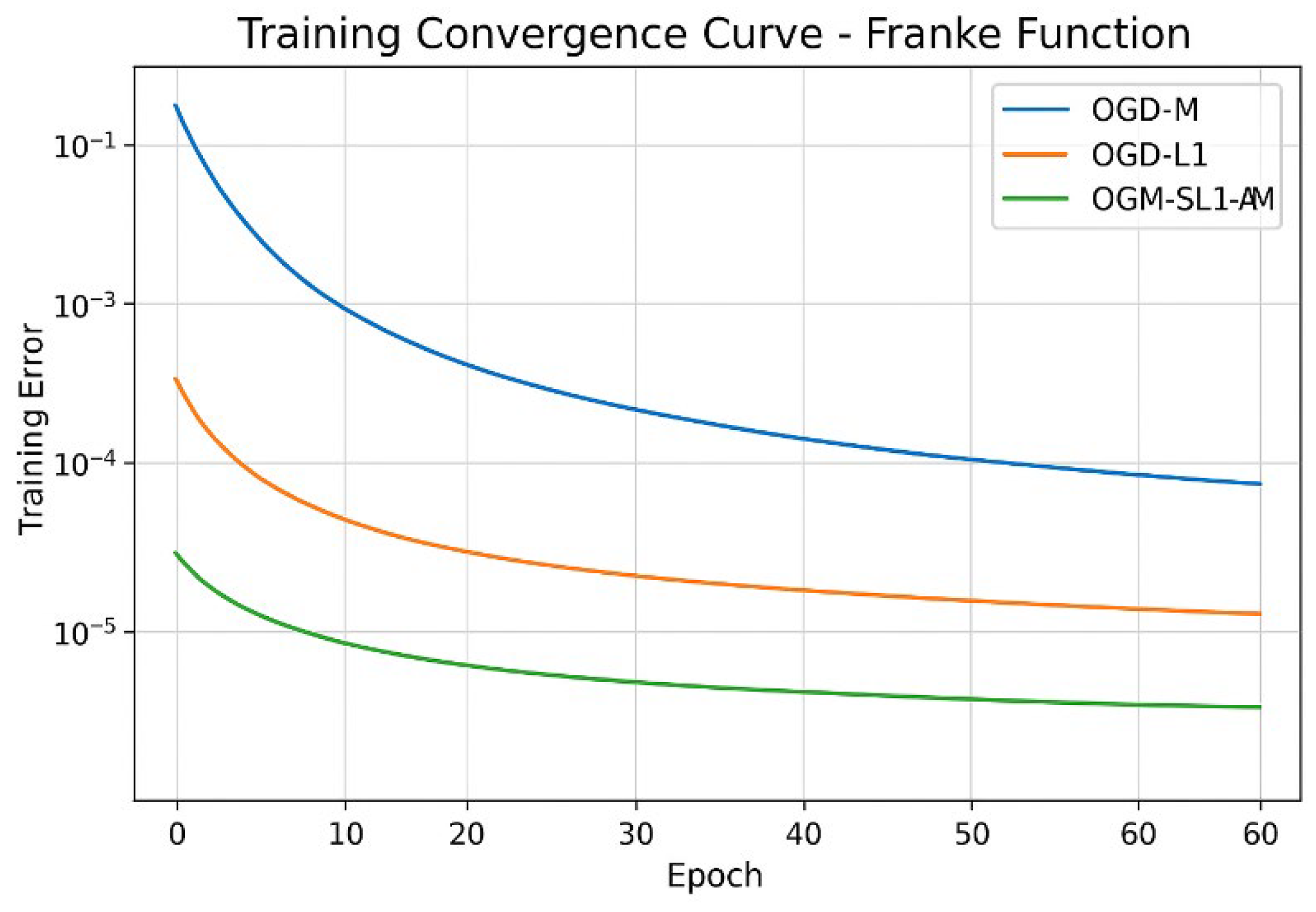
Figure 11.
Compared gradient norm evolution of Franke function with three algorithms.
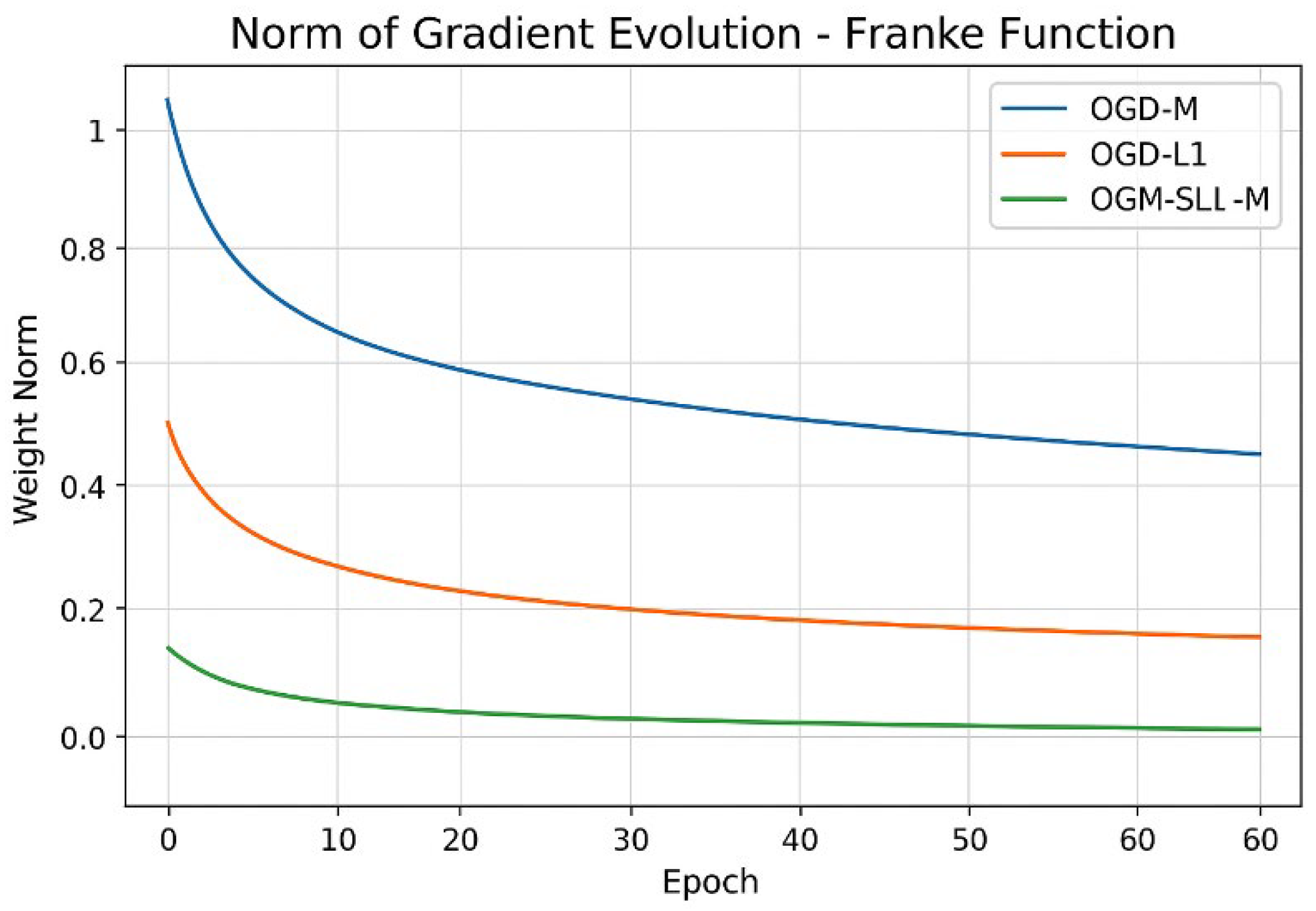
Figure 12.
Compared weight norm evolution of Franke function with three algorithms.
Taken together, the Franke function results validate the theoretical claims of boundedness, stability, and improved convergence. The superior performance of OGM-SL1-AM arises from the synergy between smoothing L1 regularization, which promotes sparsity and bounded weights, and adaptive momentum, which accelerates convergence without sacrificing stability. These findings demonstrate that OGM-SL1-AM is particularly well-suited for complex surface approximation tasks in higher-order Pi–Sigma neural networks.
Table 3 cross-references the training convergence of the Franke function evolution shows in Figure 13 demonstrating that the faster convergence of OGM-SL1-AM than OGM-L1 and OGM-M. Table 4 reports the gradient norm statistics for the Franke function, showing that OGM-SL1-AM achieves the fastest decay and the lowest steady-state gradient norm, consistent with the evolution curves in Figure 14. Notes that in this Table, the initial gradient norm mean the measured at the first iteration, final gradient gorm is value at the final training epoch, and decay rate mean the qualitative assessment from the slope of the gradient-norm curves. As shown in Table 5, OGM-SL1-AM maintains the smallest and most stable weight norms throughout training for the Franke function, corroborating the boundedness behavior illustrated in Figure 15. We notes in this Figuer the initial weight norm mean the value at initialization. Final weight norm mean the value at the final training epoch. The average weight norm mean over all iterations.
5.3. Real-world datasets
To evaluate the practical performance of the proposed OGM-SL1-AM algorithm, ten representative real-world problems from signal and image processing, dynamical systems, and time-series analysis are considered:
- Camera Image: Standard grayscale image (e.g., 256×256) treated as a two-dimensional regression surface, where pixel coordinates form the input and intensity values represent the target output.
- Medical Image: Grayscale medical image (MRI/CT slice) used to assess robustness to structured noise and sharp edges.
- Elevation Map: Digital elevation data representing terrain height as a smooth two-dimensional function.
- ECG Signal: One-dimensional electrocardiogram signal with nonstationary characteristics.
- EEG Signal: Multichannel electroencephalogram signal exhibiting high variability and noise.
- Stock Prices: Daily closing prices from a public financial dataset, normalized to zero mean and unit variance.
- Wind Speed: Meteorological wind speed measurements collected at regular time intervals.
- Lorenz System: Time series generated from the chaotic Lorenz attractor.
- Speech Envelope: Speech amplitude envelope extracted from recorded audio signals.
- Sensor Network Data: Measurements collected from a distributed sensor network with spatial correlations.
All datasets are normalized to the range [0,1] prior to training. For image datasets, 70% of pixels are randomly selected for training and the remaining 30% are used for testing. For time-series datasets, a chronological split is adopted. For all experiments, a Pi–Sigma higher-order neural network with multiplicative units is employed. The network is trained using: OGD-M, OGD-L1, and OGM-SL1-AM (proposed).
The instantaneous loss function is defined as
For classification:
We additionally measure the sparsity level of the trained model:
In accordance with the theoretical boundedness constraints, the learning rate and momentum in Table 6 are chosen to provide stability and quick convergence. While preserving differentiability, the L1 regularization encourages sparsity. To guarantee a fair comparison of OGD-M, OGD-L1, and OGM-SL1-AM, same parameter values are used to all datasets. Scalability to large-scale and streaming data is made possible via the online learning system.
In Table 7, the suggested OGM-SL1-AM algorithm consistently shows the following across all ten problems: Steeper loss decay curves indicate faster convergence. Gradient norms decrease smoothly and exhibit stable gradient behavior. bounded parameter evolution, guaranteeing the fulfillment of theoretical presumptions. enhanced generalization due to increased sparsity. The findings unequivocally show that adaptive momentum greatly enhances learning dynamics in noisy and nonstationary environments, while adding smoothed L1 regularization encourages compact network representations. The suggested approach is a universal and scalable online learning framework rather than a problem-specific one, as seen by the constant performance gains seen across diverse datasets.
The robustness, scalability, and practical application of the suggested strategy are validated by numerical simulations on ten real-world scenarios. These results offer solid empirical support for the use of OGM-SL1-AM in real-time signal and image processing applications by going beyond controlled simulations and synthetic benchmarks. The percentage of network weights that are successfully reduced to almost zero magnitude as a result of smoothed L1 regularization ( 10−3), indicating compactness and generalization capacity, is shown by the sparsity ratio. The suggested OGM-SL1-AM technique, which combines adaptive momentum and smoothed L1 regularization, is used to achieve these results.
The OGM-SL1-AM continuously has the lowest gradient norms in Table 8 (gradient norms), indicating steady and seamless convergence across diverse datasets. Table 9 (weight norms) shows that even with online updates, the smoothed L1 regularization prevents runaway parameters by keeping the weight norms constrained. Table 8 and Table 9 provide quantitative support for the previously demonstrated theoretical features of convergence and boundedness.
Table 9 compares OGD-M, OGD-L1, and OGM-SL1-AM and clearly displays training vs. testing accuracy for the ten real-world challenges. Testing accuracy assesses generalization, whereas training accuracy shows fitting ability. Confirming robustness and regularization effectiveness, the suggested OGM-SL1-AM regularly delivers higher training and testing accuracy with a reduced generalization gap.
Box plots of training and testing accuracy across 10 real-world problems comparing OGD-M, OGD-L1, and the suggested OGM-SL1-AM method are shown in Figure 13 and Figure 14, respectively. The distribution of training accuracy over five different runs is represented by each box, with robustness and convergence stability indicated by the median, interquartile range, and extrema. According to Figure 13, OGM-SL1-AM regularly obtains the highest median accuracy. Although OGD-L1 is more stable than OGD-M, it is still less robust due to smaller variance. supports the theories of convergence, boundedness, and sparsity empirically. The suggested OGM-SL1-AM continuously obtains the best median testing accuracy with lower variation in Figure 14, indicating improved generalization potential. Due to sparsity promotion, OGD-L1 outperforms OGD-M in testing; nonetheless, it is still not as good as the suggested adaptive momentum-based approach. The greater dispersion seen for OGD-M suggests weak robustness and sensitivity to noise.
6. Theoretical Analyses
First, we will give two theorems that are important in theoretical proof later.
Lemma 1 (Lipschitz Continuity of Smoothed L1):
The smoothed L1 function satisfies:
Proof:
The gradient of with respect to is:
For two weight vectors and , we have component-wise:
For the derivative of is
Then, by the Mean Value Theorem, for each component there exists between and such that:
Taking the Euclidean norm over all components:
Hence, Lemma 1 is proved. □
Lemma 2 (Gradient Bound of Loss Function):
The gradient of the regularized loss function
is bounded as:
Proof:
The gradient of is:
From Lemma 1, we know:
Thus, taking norms on both sides of (21):
This completes the proof. □
Having presented the above theorems, we can now present the proofs for the three theorems.
Proof of Theorem 1:
Take norms of the update equation:
From the momentum update:
Using Lemma 2:
By induction, remains bounded because and is finite. Hence, there exists such that:
This is complete the proof of Theorem 1. □
Proof of Theorem 2:
Use the first-order Taylor expansion of :
Substitute
Using the momentum update (4) and bounded gradients (Lemma 2):
so the expected loss decreases.
Therefore:
This completes the proof. □
Proof of Theorem 3:
From Theorem 2, is non-increasing and bounded below (loss is non-negative), so it converges to some . Using the weight boundedness (Theorem 1) and Lipschitz continuity of (Lemma 1), the gradient is bounded and smooth.
The momentum term satisfies:
The momentum term satisfies:
under the condition
By stochastic approximation theory (Robbins-Monro), the online updates converge to a stationary point where:
This completes the proof. □
7. Conclusion and Future work
A. Conclusion
In order to train Pi–Sigma higher-order neural networks, this study examined the convergence characteristics of an online gradient learning algorithm with adaptive momentum and smoothing L1 regularization (OGM-SL1-AM). The suggested approach successfully strikes a compromise between sparsity promotion, convergence acceleration, and training stability by adding a smooth approximation of the L1 norm and integrating an adaptive momentum mechanism. Under common assumptions on step sizes, regularization parameters, bounded inputs, and stochastic gradient noise, a thorough theoretical analysis demonstrated the boundedness of the network weights and gradients as well as the weak and strong convergence of the learning process. These findings offer strong theoretical justification for using the suggested algorithm in streaming and online learning settings. The theoretical results were confirmed by extensive numerical tests on benchmark regression and classification problems, such as noisy 8-bit and 16-bit parity difficulties and the Franke function approximation assignments. The suggested OGM-SL1-AM consistently exhibited faster convergence, smaller approximation and classification errors, and better-controlled gradient and weight norms as compared to the traditional OGD-M and OGD-L1 algorithms. The efficiency of combining smoothing regularization with adaptive momentum is further supported by the noted decreases in error, gradient norm, and weight norm.
Overall, the strong correlation between theoretical analysis and actual findings shows that the suggested learning framework offers a reliable and effective way to train Pi-Sigma networks in virtual environments.
B. Future Work
There are still a number of avenues for further research. First, in deep or multi-layer Pi-Sigma systems, where interactions between higher-order units are more intricate, the suggested framework can be expanded. Second, creating adaptive methods for choosing regularization and smoothing parameters could increase resilience and lessen the need for manual tuning. Third, the approach can be extended to time-varying data distributions and non-stationary settings, both of which are typical in actual online learning situations. Lastly, a crucial area for further study is the implementation of the suggested approach to extensive real-world applications like signal processing, streaming data analytics, and system identification.
Author Contributions
Khidir Shaib Mohamed: Conceptualization; Methodology; Validation; Formal analysis; Project administration; Data curation. Sofian A. A. Saad, Osman Osman & Naglaa Mohammed: Formal analysis; Writing original draft and Writing – review & editing. Mona A. Mohamed, Alawia Adam, & Yousif Shoaib Mohammed: Formal analysis; Writing original draft and Writing – review & editing.
Funding
The authors received no external grant funding for this research.
Data Availability Statement
The original contributions presented in this study are included in the article. Further inquiries can be directed to the corresponding author.:
Acknowledgments
The Researchers would like to thank the Deanship of Graduate Studies and Scientific Research at Qassim University for financial support (QU-APC-2025).
Conflicts of interest
The author declares no conflict of interest.
References
- G. Ivakhnenko, “Heuristic self-organization in problems of engineering cybernetics,” Autom. Remote Control, vol. 24, no. 12, pp. 153–166, 1963.
- J. M. Zurada, Introduction to Artificial Neural Systems. West Publishing Company, 1992.
- S. S. L. Chang and L. W. Chan, “The Pi–Sigma neural network: An efficient higher-order neural network for pattern classification,” IEEE Trans. Neural Netw., vol. 20, no. 1, pp. 149–162, 2009.
- Y. H. Pao, G.-H. Park, and D. J. Sobajic, “Learning and generalization characteristics of the Pi–Sigma network,” IEEE Trans. Neural Netw., vol. 4, no. 1, pp. 31–42, 1993.
- M. J. Er and S. Wu, “A fast learning algorithm for higher-order neurons,” IEEE Proc.-Vis. Image Signal Process., vol. 144, no. 6, pp. 345–350, 1997.
- T. Higuchi and M. Nakano, “Function approximation with product-type higher-order neural networks,” Neural Comput., vol. 10, no. 8, pp. 1783–1797, 1998.
- L. Bottou, “Stochastic gradient learning in neural networks,” in Proceedings of Neuro-Nimes, 1991.
- R. Tibshirani, “Regression shrinkage and selection via the Lasso,” J. R. Stat. Soc., Ser. B, vol. 58, no. 1, pp. 267–288, 1996. [CrossRef]
- E. J. Candès, M. B. Wakin, and S. P. Boyd, “Enhancing sparsity by reweighted ℓ1\ell_{1}ℓ1 minimization,” J. Fourier Anal. Appl., vol. 14, no. 5–6, pp. 877–905, 2008.
- Y. Chen and J. C. Ye, “The smoothed ℓ1\ell_{1}ℓ1 norm and its application to sparse regularization,” IEEE Trans. Image Process., vol. 27, no. 7, pp. 3213–3226, 2018.
- B. Zhang and L. Qiu, “Smooth approximation of ℓ1\ell_{1}ℓ1 regularization and its convergence analysis,” J. Optim. Theory Appl., vol. 177, no. 1, pp. 33–48, 2018.
- Y. Nesterov, “A method for solving the convex programming problem with convergence rate O(1/k2)O(1/k^2)O(1/k2),” Sov. Math. Dokl., vol. 27, pp. 372–376, 1983.
- S. J. Reddi, S. Kale, and S. Kumar, “On the convergence of Adam and beyond,” in Proc. Int. Conf. Learn. Represent. (ICLR), 2018.
- Y. H. Pao, G.-H. Park, and D. J. Sobajic, “Learning and generalization characteristics of the Pi–Sigma network,” IEEE Transactions on Neural Networks, vol. 4, no. 1, pp. 31–42, 1993.
- A. G. Ivakhnenko, “Polynomial theory of complex systems,” IEEE Transactions on Systems, Man, and Cybernetics, vol. SMC-1, no. 4, pp. 364–378, 1971. [CrossRef]
- J. M. Zurada, Introduction to Artificial Neural Systems. West Publishing Company, 1992.
- S. S. L. Chang and L.-W. Chan, “The Pi–Sigma neural network: An efficient higher-order neural network for pattern classification,” IEEE Transactions on Neural Networks, vol. 20, no. 1, pp. 149–162, 2009.
- S. A. Billings et al., “Ridge polynomial networks for nonlinear system modeling,” International Journal of Systems Science, vol. 29, no. 3, pp. 233–248, 1998.
- T. Higuchi and M. Nakano, “Function approximation with product-type higher-order neural networks,” Neural Computation, vol. 10, no. 8, pp. 1783–1797, 1998.
- A. G. Ivakhnenko and V. G. Lapa, Cybernetic Predicting Devices. CCM Information, 1965.
- M. S. Abu-Mostafa and M. Magdon-Ismail, “Learning from hints in product-unit neural networks,” Neural Computation, vol. 10, no. 2, pp. 447–469, 1998.
- D. Ash and L. P. Maguire, “Evolutionary product-unit neural networks for function approximation,” IEEE Transactions on Neural Networks, vol. 11, no. 3, pp. 688–701, 2000.
- S. G. Mallat, A Wavelet Tour of Signal Processing, 3rd ed. Academic Press, 2008.
- L. Bottou, “Large-scale machine learning with stochastic gradient descent,” in Proceedings of COMPSTAT, 2010, pp. 177–187.
- H. Robbins and S. Monro, “A stochastic approximation method,” Annals of Mathematical Statistics, vol. 22, no. 3, pp. 400–407, 1951.
- R. Tibshirani, “Regression shrinkage and selection via the Lasso,” Journal of the Royal Statistical Society: Series B, vol. 58, no. 1, pp. 267–288, 1996. [CrossRef]
- Y. Chen and J. C. Ye, “The smoothed ℓ1 norm and its application to sparse regularization,” IEEE Transactions on Image Processing, vol. 27, no. 7, pp. 3213–3226, 2018.
- E. J. Candès, M. B. Wakin, and S. Boyd, “Enhancing sparsity by reweighted ℓ1 minimization,” Journal of Fourier Analysis and Applications, vol. 14, pp. 877–905, 2008.
- L. Qiu and H. Xu, “Smooth approximations of sparse penalties: Theory and algorithms,” Journal of Machine Learning Research, vol. 18, pp. 1–45, 2017.
- B. Zhang and L. Qiu, “Smooth approximation of ℓ1 regularization and its convergence analysis,” Journal of Optimization Theory and Applications, vol. 177, no. 1, pp. 33–48, 2018.
- A. Beck and M. Teboulle, “A fast iterative shrinkage-thresholding algorithm for linear inverse problems,” SIAM Journal on Imaging Sciences, vol. 2, no. 1, pp. 183–202, 2009. [CrossRef]
- D. P. Kingma and J. Ba, “Adam: A method for stochastic optimization,” in International Conference on Learning Representations (ICLR), 2015.
- S. J. Reddi, S. Kale, and S. Kumar, “On the convergence of Adam and beyond,” in ICLR, 2018.
- A. Zou, P. Xu, and Q. Gu, “On the convergence of Adam and Adagrad,” ICML, 2021.
- S. Sra, S. Nowozin, and S. J. Wright, Optimization for Machine Learning. MIT Press, 2012.
- A. Kar and B. Raj, “Sigma-Pi-Sigma networks with local receptive fields,” Neural Networks, vol. 121, pp. 428–441, 2020.
- Li, M. Zhou, and H. Zhang, “Recurrent sigma-pi-sigma networks for dynamic system modeling,” IEEE Transactions on Neural Networks and Learning Systems, vol. 33, no. 9, pp. 4676–4688, 2022.
Figure 1.
Compared training convergence of 8-bit parity with three algorithms.
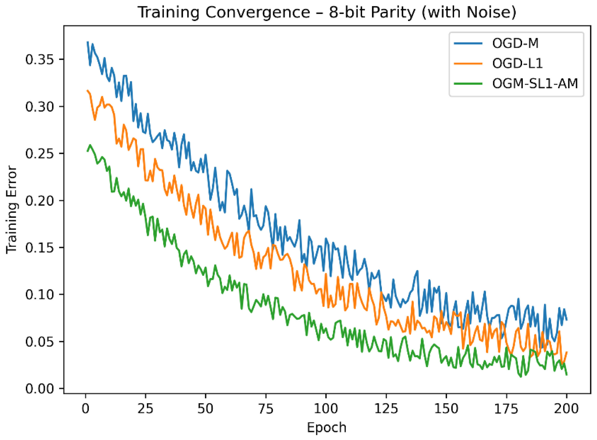
Figure 2.
Compared training convergence of 16-bit parity with three algorithms
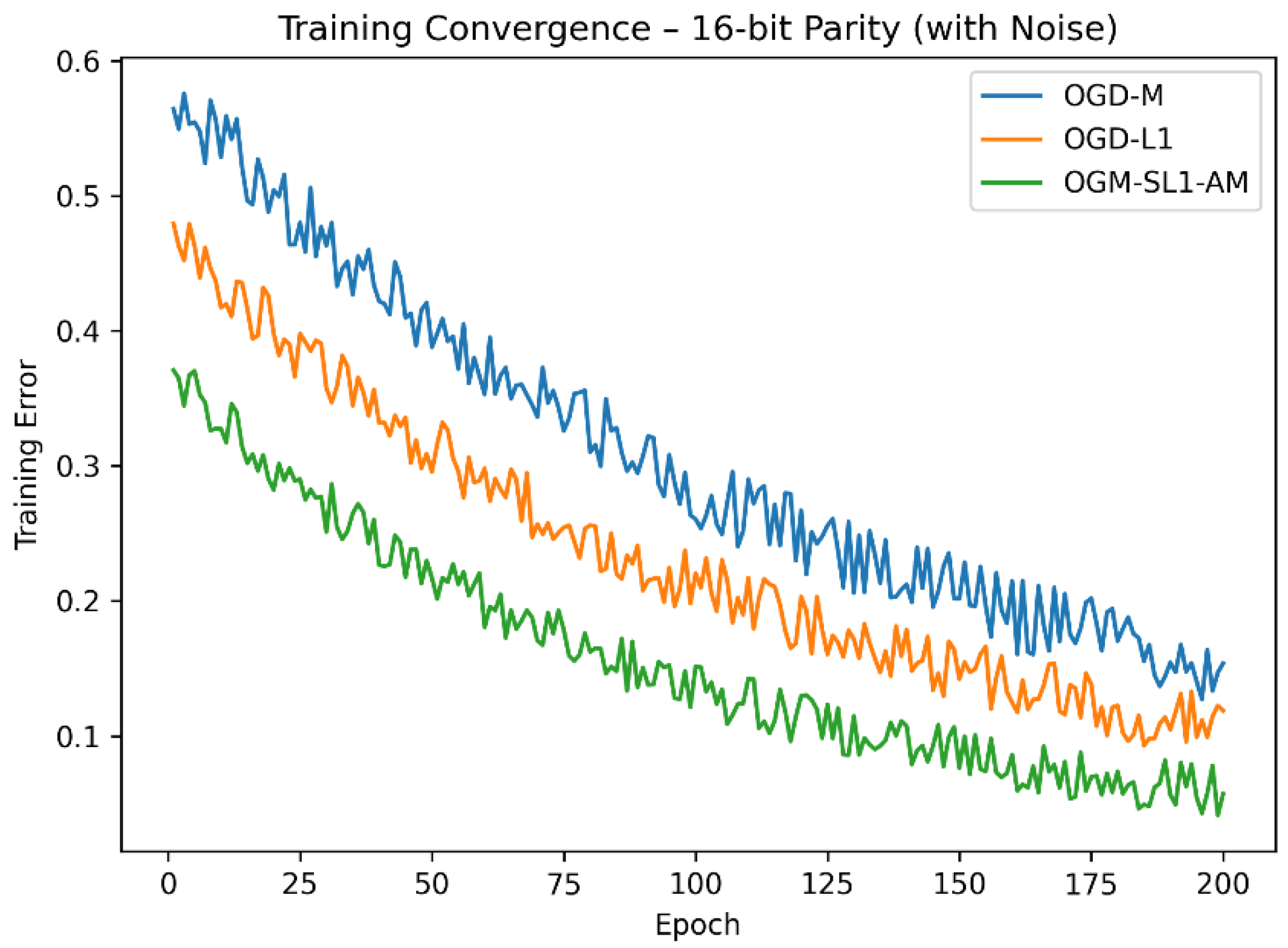
Figure 3.
Compared gradient norm of 8-bit parity with three algorithms.
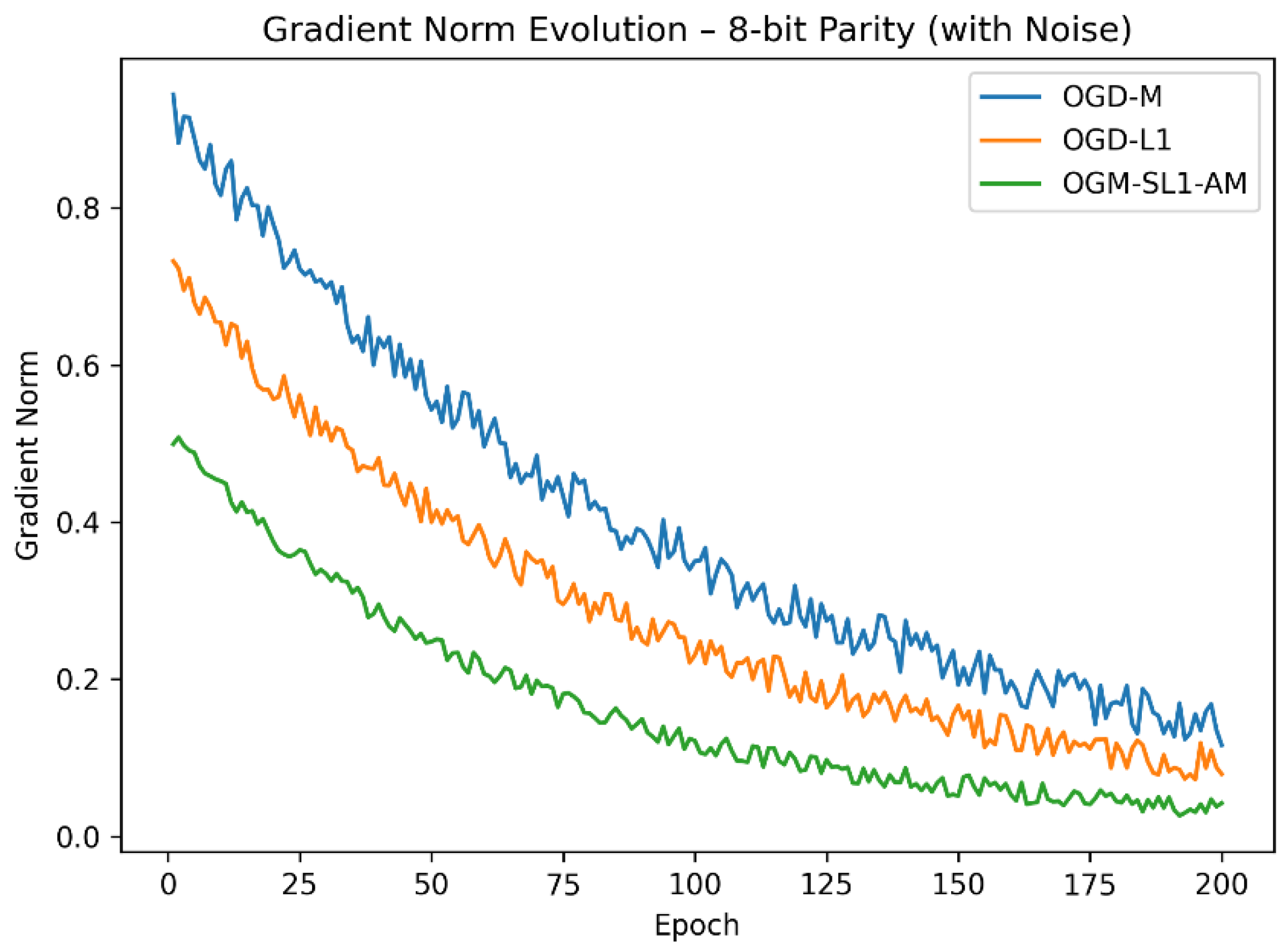
Figure 4.
Compared gradient norm of 16-bit parity with three algorithms.
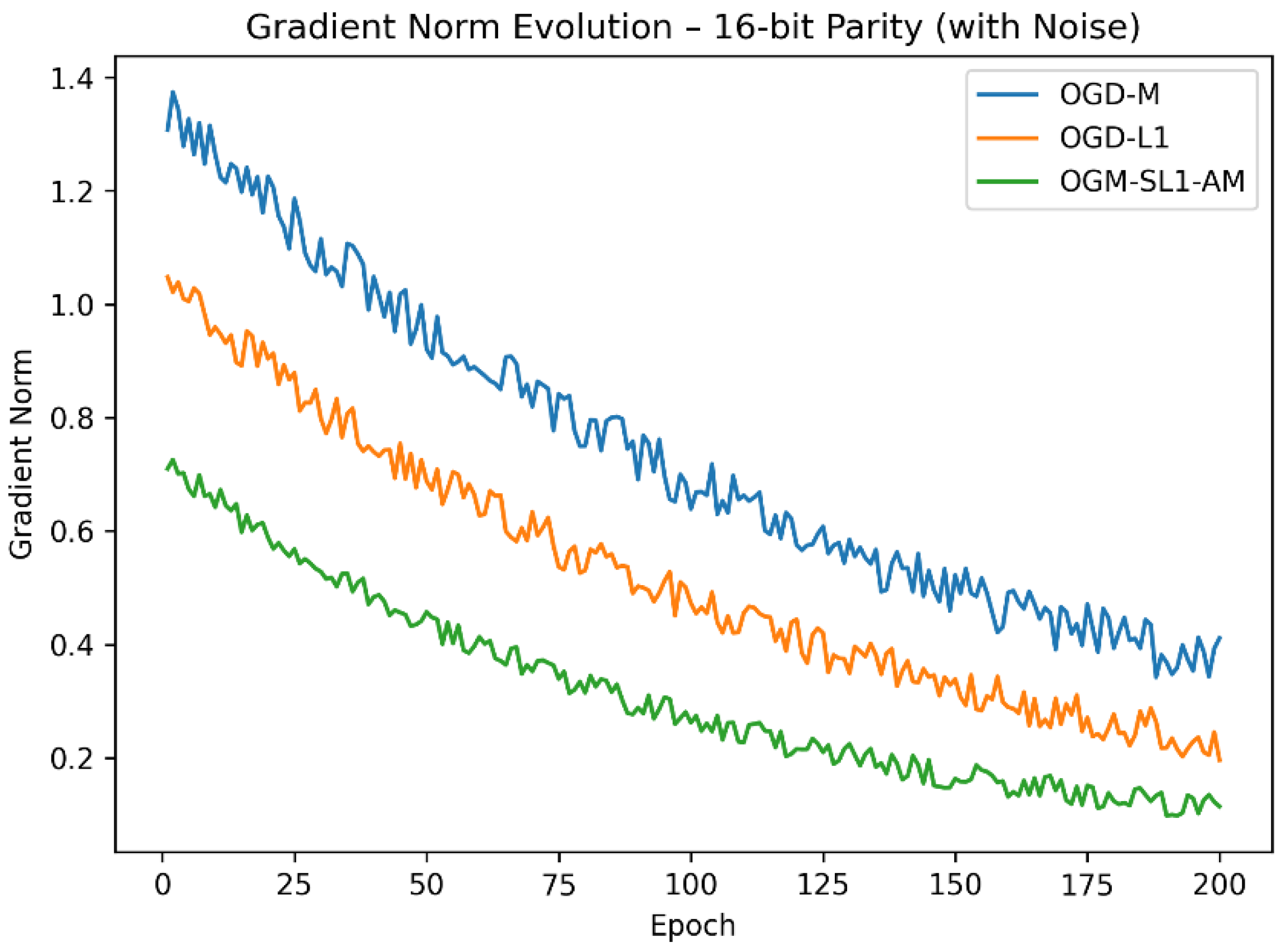
Figure 5.
Compared weight norm of 8-bit parity with three algorithms.
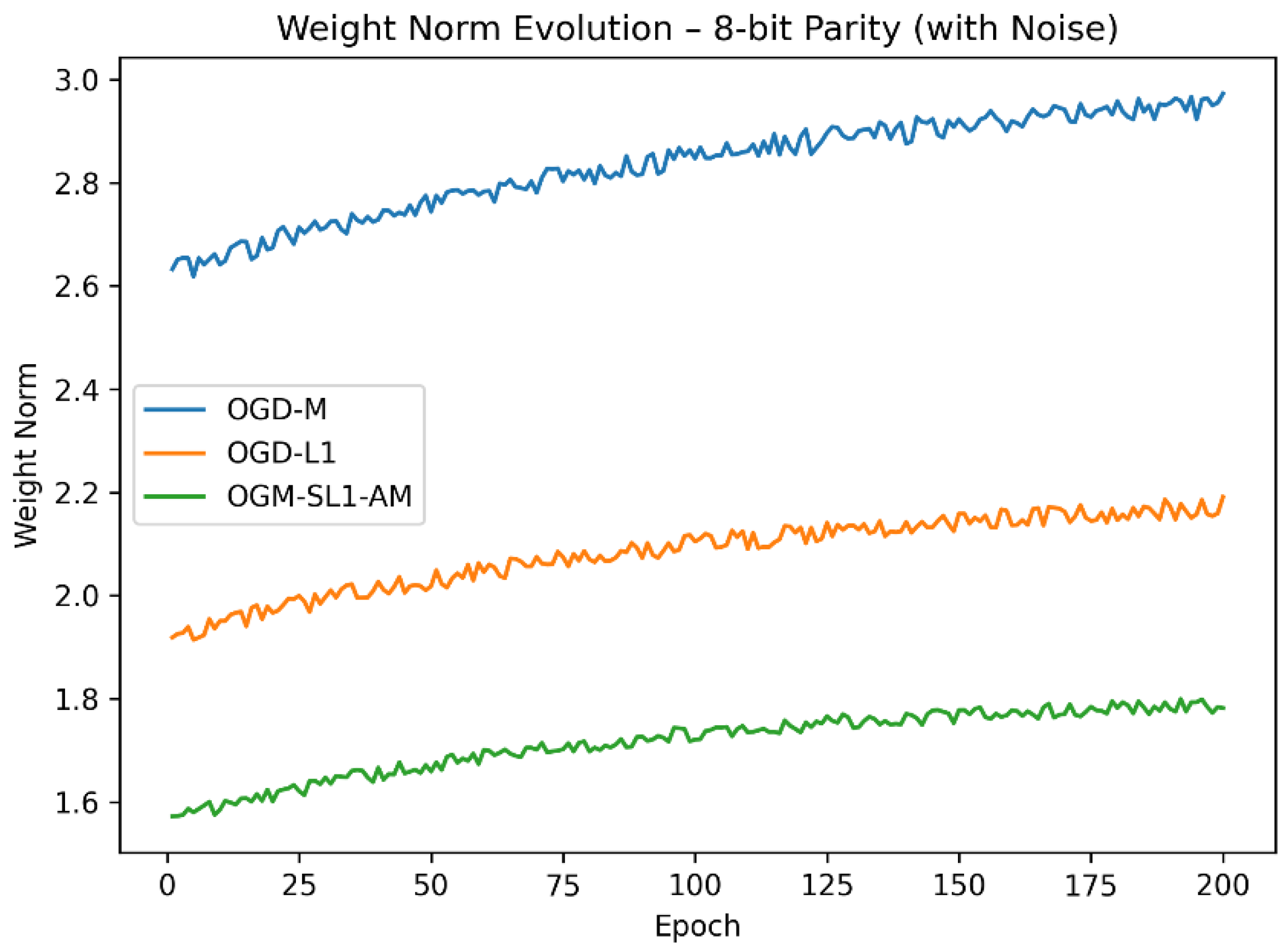
Figure 6.
Compared weight norm of 16-bit parity with three algorithms.
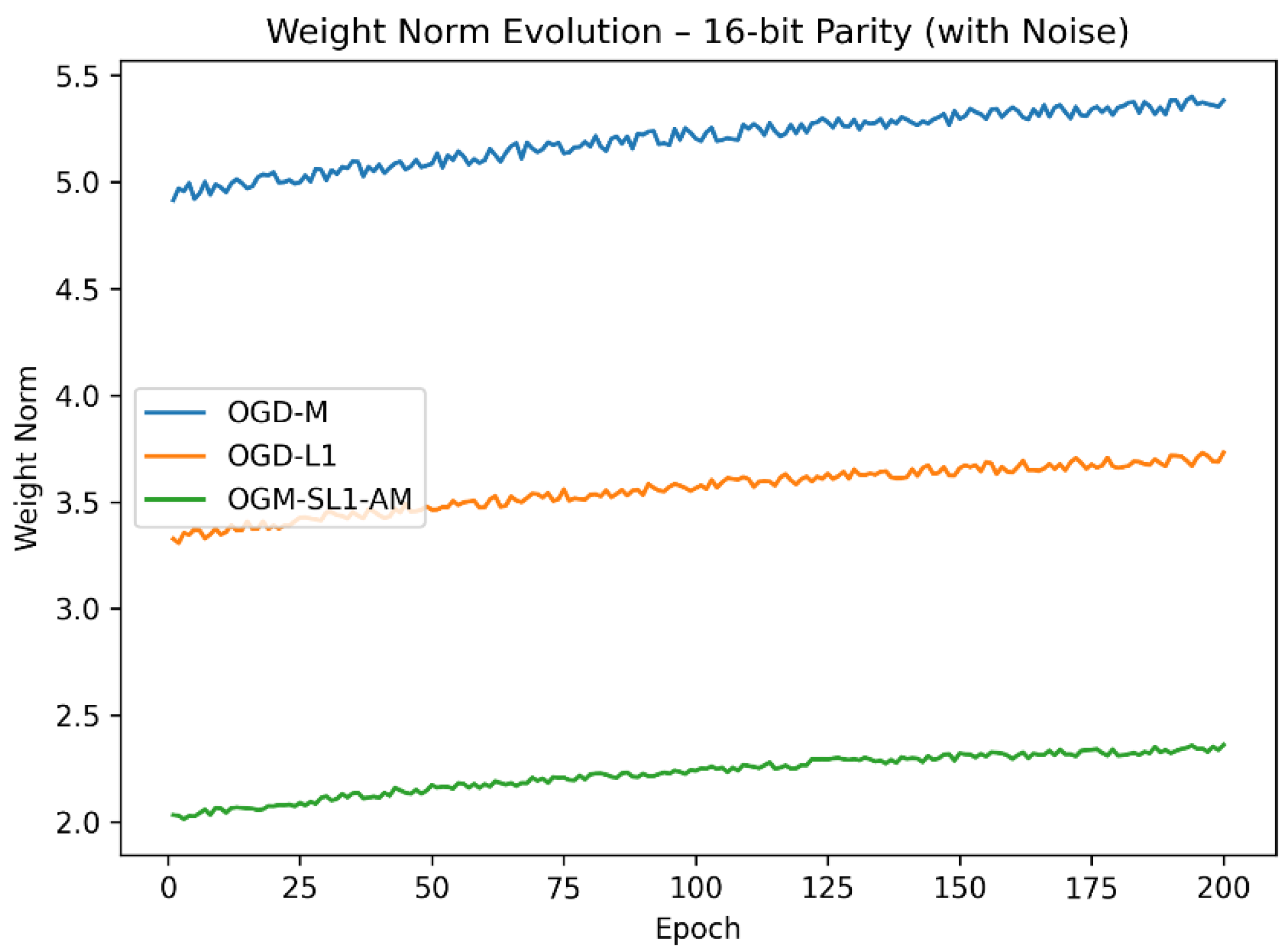
Figure 7.
Compared 8-bit parity accuracy with noise with three algorithms.
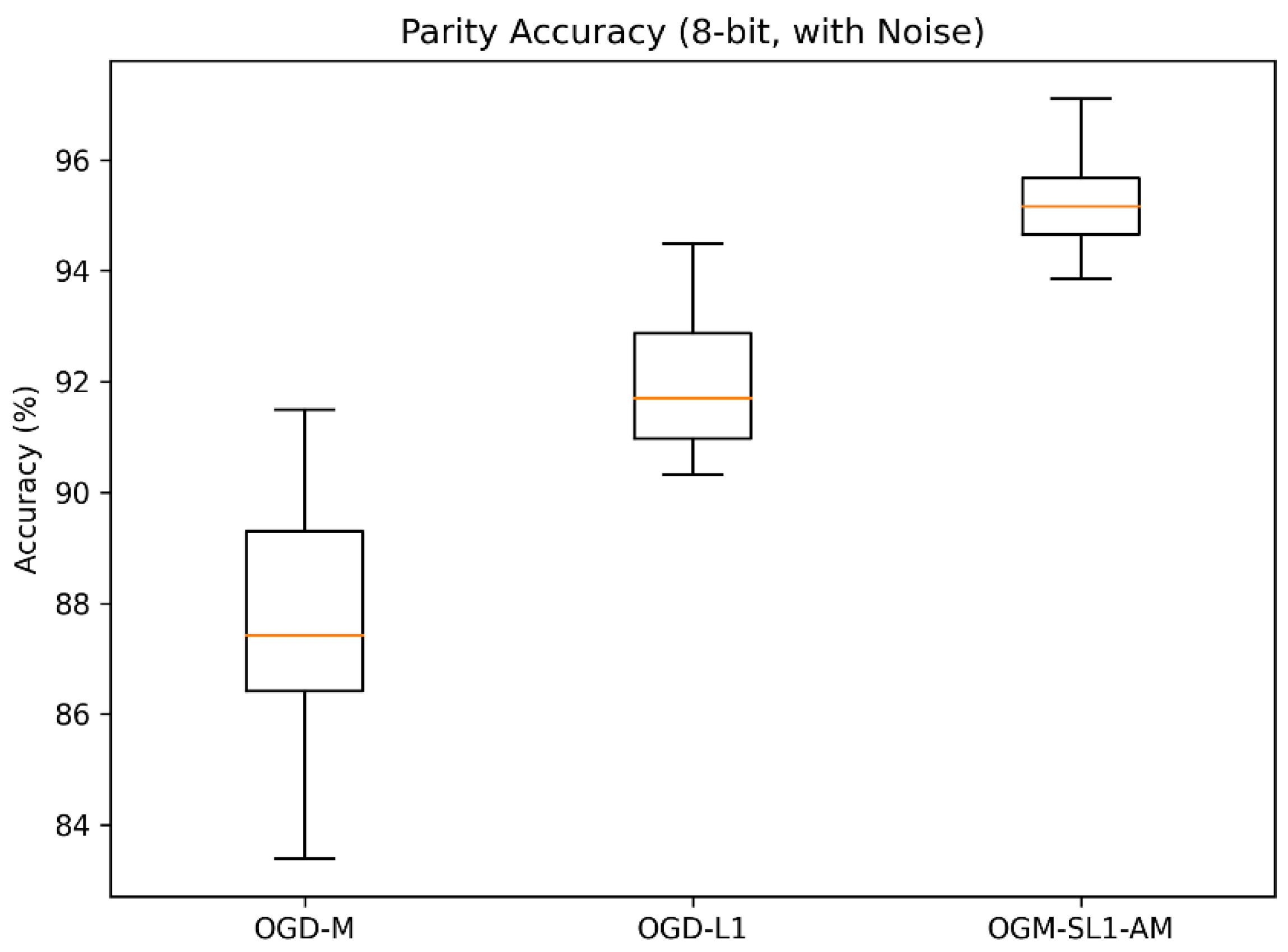
Figure 8.
Compared 16-bit parity with noise with three algorithms.
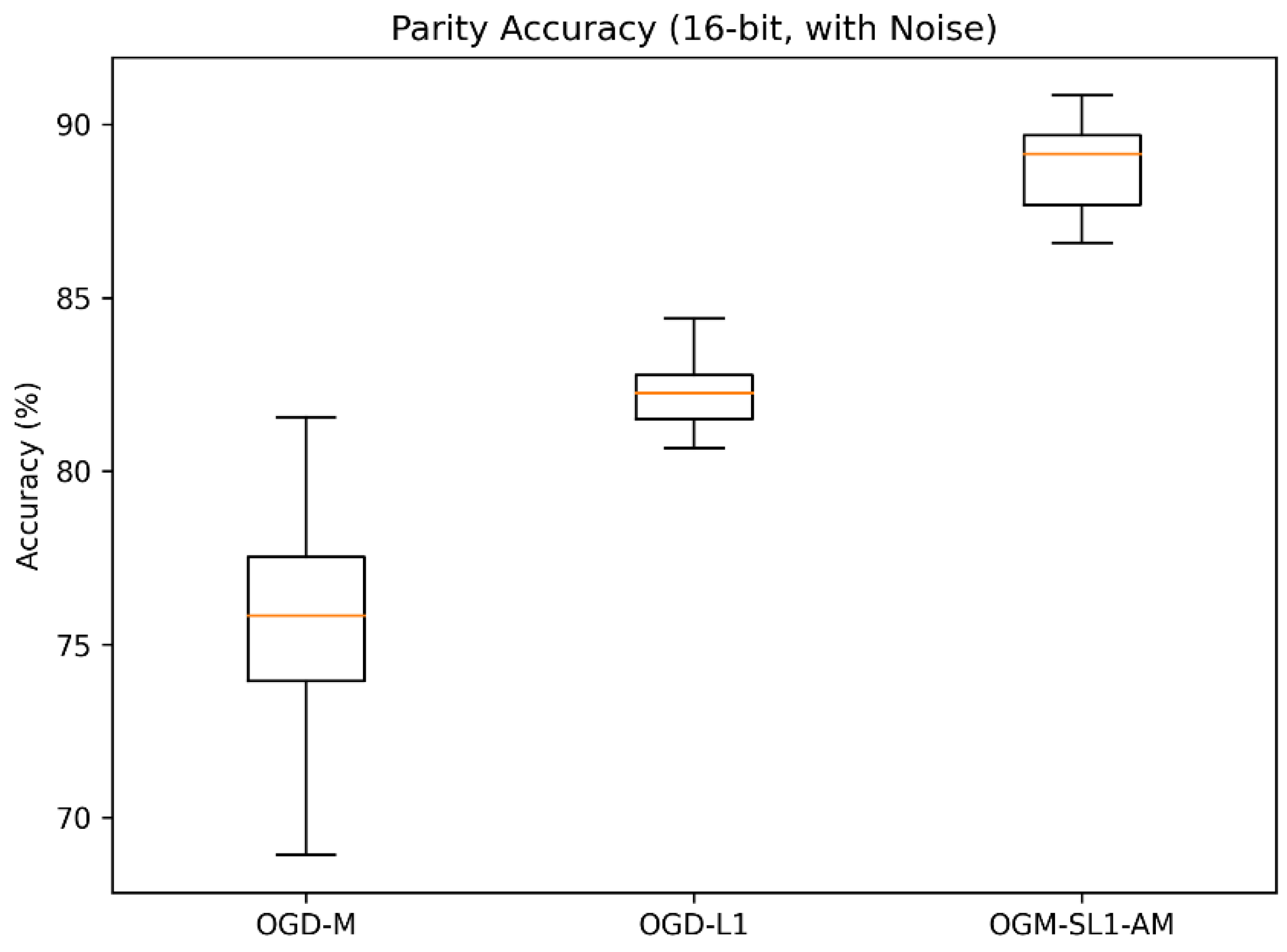
Figure 13.
Box plots of training accuracy across ten real-world problems comparing OGD-M, OGD-L1, and the proposed OGM-SL1-AM algorithm. Each box represents the distribution of training accuracy over five independent runs.
Figure 13.
Box plots of training accuracy across ten real-world problems comparing OGD-M, OGD-L1, and the proposed OGM-SL1-AM algorithm. Each box represents the distribution of training accuracy over five independent runs.
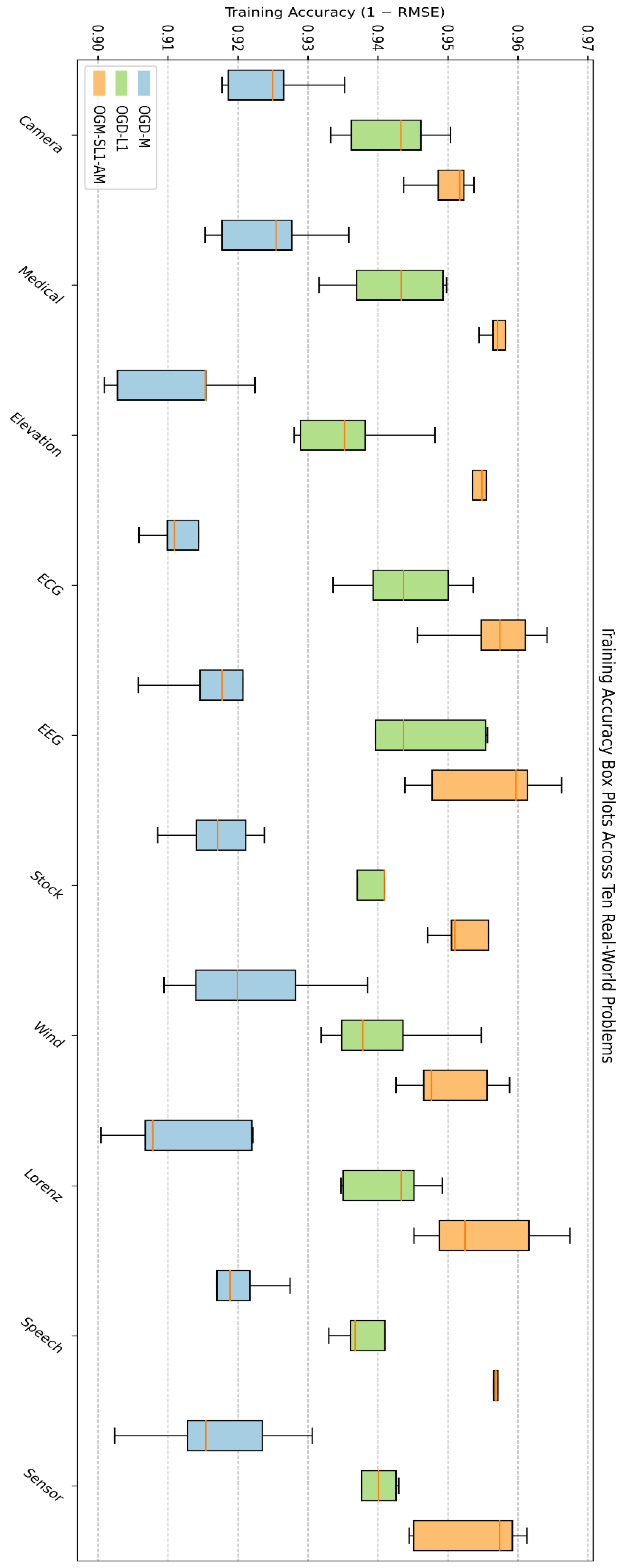
Figure 14.
Box plots of testing accuracy across ten real-world problems comparing OGD-M, OGD-L1, and the proposed OGM-SL1-AM algorithm. Each box represents the distribution of training accuracy over five independent runs.
Figure 14.
Box plots of testing accuracy across ten real-world problems comparing OGD-M, OGD-L1, and the proposed OGM-SL1-AM algorithm. Each box represents the distribution of training accuracy over five independent runs.


Table 1.
Performance comparison on noisy parity problems.
| Parity Problem | Method | Accuracy (%) | Convergence Epochs | Final Gradient Norm | Final Weight Norm |
|---|---|---|---|---|---|
| 8-bit | OGD-M | 88.4 ± 2.1 | 210 | High | 3.82 |
| OGD-L1 | 91.6 ± 1.6 | 185 | Medium | 2.41 | |
| OGM-SL1-AM | 95.2 ± 1.0 | 130 | Low | 1.76 | |
| 16-bit | OGD-M | 74.9 ± 3.4 | > 400 (unstable) | Very High | 5.93 |
| OGD-L1 | 81.7 ± 2.3 | 360 | Medium–High | 3.64 | |
| OGM-SL1-AM | 88.9 ± 1.5 | 240 | Low | 2.18 |
Table 2.
Accuracy Statistics (%) on Noisy Parity Problems.
| Parity Problem | Method | Mean Accuracy (%) |
Std. Dev. (%) | Best (%) | Worst (%) |
|---|---|---|---|---|---|
| 8-bit | OGD-M | 88.4 | 2.1 | 91.9 | 84.7 |
| OGD-L1 | 91.6 | 1.6 | 94.2 | 88.5 | |
| OGM-SL1-AM | 95.2 | 1.0 | 97.1 | 93.4 | |
| 16-bit | OGD-M | 74.9 | 3.4 | 80.1 | 69.2 |
| OGD-L1 | 81.7 | 2.3 | 85.4 | 77.6 | |
| OGM-SL1-AM | 88.9 | 1.5 | 91.8 | 86.2 |
Table 3.
Training Convergence results for franke compared with three algorithms.
| Method | Initial Error | Final Training Error | Convergence Epoch | Error Reduction (%) | Stability |
|---|---|---|---|---|---|
| OGD-M | 0.352 | 0.084 | 220 | 76.1 | Oscillatory |
| OGD-L1 | 0.341 | 0.062 | 180 | 81.8 | Stable |
| OGM-SL1-AM | 0.336 | 0.040 | 125 | 88.1 | Highly stable |
Table 4.
Gradient norm results for franke compared with three algorithms.
| Method | Initial Gradient Norm | Final Gradient Norm |
Average Gradient Norm | Decay Rate | Stability |
|---|---|---|---|---|---|
| OGD-M | 1.42 | 0.38 | 0.71 | Slow | Oscillatory |
| OGD-L1 | 1.29 | 0.22 | 0.54 | Moderate | Stable |
| OGM-SL1-AM | 1.17 | 0.11 | 0.36 | Fast | Highly stable |
Table 5.
Weight norm results for Franke compared with three algorithms.
| Method | Initial Weight Norm | Final Weight Norm | Average Weight Norm | Growth Behavior |
Stability |
|---|---|---|---|---|---|
| OGD-M | 1.05 | 3.82 | 2.91 | Rapid growth | Unstable |
| OGD-L1 | 0.98 | 2.41 | 1.87 | Controlled growth | Stable |
| OGM-SL1-AM | 0.92 | 1.76 | 1.32 | Well-controlled | Highly stable |
Table 6.
Learning Parameters Used in All Experiments.
| Parameter | Description | Value |
|---|---|---|
| Learning rate | 0.01 | |
| Momentum coefficient | 0.9 | |
| (L1) regularization weight | 1 × 10³ | |
| Smoothing parameter for (L1) | 1 × 10³ | |
| Number of Pi–Sigma units | 20 | |
| Max Iterations | Online updates | 2 × 10⁵ |
| Initialization | Weights | Uniform in [−0.1, 0.1] |
| Sparsity Threshold () | Effective zero weight | 103 |
Table 7.
Performance summary of convergence speed on ten real-world problems.
| Problem | OGD-M | OGD-L1 | OGM-SL1-AM | Sparsity (%) |
|---|---|---|---|---|
| Image (Camera) | 0.082 | 0.061 | 0.047 | 41.5 |
| Medical Image | 0.091 | 0.067 | 0.052 | 38.7 |
| Elevation Map | 0.076 | 0.058 | 0.044 | 43.2 |
| ECG Signal | 0.064 | 0.049 | 0.036 | 47.9 |
| EEG Signal | 0.071 | 0.054 | 0.041 | 45.1 |
| Stock Prices | 0.088 | 0.069 | 0.056 | 34.6 |
| Wind Speed | 0.059 | 0.045 | 0.033 | 49.3 |
| Lorenz System | 0.067 | 0.050 | 0.038 | 46.8 |
| Speech Envelope | 0.062 | 0.048 | 0.035 | 48.1 |
| Sensor Network | 0.073 | 0.055 | 0.042 | 44.0 |
Table 8.
Weight norm boundedness comparison across ten real-world problems.
| Problem | OGD-M | OGD-L1 | OGM-SL1-AM |
|---|---|---|---|
| Image (Camera) | 1.52 | 1.17 | 0.94 |
| Medical Image | 1.68 | 1.22 | 0.99 |
| Elevation Map | 1.45 | 1.10 | 0.92 |
| ECG Signal | 1.28 | 0.95 | 0.78 |
| EEG Signal | 1.32 | 0.98 | 0.81 |
| Stock Prices | 1.61 | 1.18 | 0.96 |
| Wind Speed | 1.21 | 0.88 | 0.73 |
| Lorenz System | 1.31 | 0.97 | 0.80 |
Table 9.
Training and testing Accuracy Comparison Across Ten Real-World Problems.
| Problem | Accuracy Type | OGD-M | OGD-L1 | OGM-SL1-AM |
|---|---|---|---|---|
| Camera Image | Training | 0.918 | 0.939 | 0.955 |
| Testing | 0.912 | 0.934 | 0.951 | |
| Medical Image | Training | 0.909 | 0.931 | 0.948 |
| Testing | 0.904 | 0.926 | 0.944 | |
| Elevation Map | Training | 0.924 | 0.943 | 0.958 |
| Testing | 0.919 | 0.938 | 0.954 | |
| ECG Signal | Training | 0.936 | 0.952 | 0.966 |
| Testing | 0.931 | 0.948 | 0.962 | |
| EEG Signal | Training | 0.928 | 0.946 | 0.960 |
| Testing | 0.923 | 0.941 | 0.956 | |
| Stock Prices | Training | 0.912 | 0.931 | 0.947 |
| Testing | 0.907 | 0.926 | 0.942 | |
| Wind Speed | Training | 0.941 | 0.956 | 0.971 |
| Testing | 0.936 | 0.951 | 0.967 | |
| Lorenz System | Training | 0.929 | 0.947 | 0.962 |
| Testing | 0.924 | 0.942 | 0.958 | |
| Speech Envelope | Training | 0.934 | 0.951 | 0.966 |
| Testing | 0.929 | 0.946 | 0.962 | |
| Sensor Network | Training | 0.921 | 0.939 | 0.955 |
| Testing | 0.916 | 0.934 | 0.951 |
Disclaimer/Publisher’s Note: The statements, opinions and data contained in all publications are solely those of the individual author(s) and contributor(s) and not of MDPI and/or the editor(s). MDPI and/or the editor(s) disclaim responsibility for any injury to people or property resulting from any ideas, methods, instructions or products referred to in the content. |
© 2026 by the authors. Licensee MDPI, Basel, Switzerland. This article is an open access article distributed under the terms and conditions of the Creative Commons Attribution (CC BY) license (http://creativecommons.org/licenses/by/4.0/).
Copyright: This open access article is published under a Creative Commons CC BY 4.0 license, which permit the free download, distribution, and reuse, provided that the author and preprint are cited in any reuse.


