Submitted:
16 June 2024
Posted:
17 June 2024
You are already at the latest version
Abstract
Gradients of smooth functions with non-independent variables are relevant for exploring complex models and for the optimization of functions subjected to constraints. In this paper, we investigate new and simple approximations and computations of such gradients by making use of independent, central and symmetric variables. Such approximations are well-suited for applications in which the computations of the gradients are too expansive or impossible. The derived upper-bounds of the biases of our approximations do not suffer from the curse of dimensionality for any $2$-smooth function, and theoretically improve the known results. Also, our estimators of such gradients reach the optimal (mean squared error) rate of convergence (i.e., $\mathcal{O}(N^{-1})$) for the same class of functions. Numerical comparisons based on a test case and a high-dimensional PDE model show the efficiency of our approach.
Keywords:
Dependent variables
; Gradients
; High-dimensional models
; Optimal estimators
; Tensor metric of non-independent inputs
1. Introduction
Non-independent variables arise when at least two variables do not vary independently, and such variables are often characterized by their covariance matrices, distribution functions, copulas, weighted distributions (see e.g., [1,2,3,4,5,6,7]). Recently, dependency models provide explicit functions that link these variables together by means of additional independent variables ([8,9,10,11,12]). Models with non-independent input variables, including functions subjected to constraints, are widely encountered in different scientific fields, such as data analysis, quantitative risk analysis, and uncertainty quantification (see e.g., [13,14,15]).
Analyzing such functions requires being able to calculate or to compute their dependent gradients, that is, the gradients that account for the dependencies among the inputs. Recall that gradients are involved in i) inverse problems and optimization (see e.g., [16,17,18,19,20]), ii) exploring complex mathematical models or simulators (see [21,22,23,24,25,26,27,28] for independent inputs and [9,15] for non-independent variables); iii) Poincaré inequalities and equalities ([9,28,29,30]), and recently in iv) derivative-based ANOVA (i.e., exact expansions) of functions ([28]). While the first-order derivatives of functions with non-independent variables have been derived in [9] for screening dependent inputs of high-dimensional models, the theoretical expressions of the gradients of such functions (dependent gradients) have been introduced in [15], enhancing the difference between the gradients and the first-order partial derivatives when the input variables are dependent or correlated.
In high-dimensional settings and for time-demanding models, having an efficient approach for computing the dependent gradients provided in [15] using a few model evaluations is worth investigating. So far, the adjoint methods can provide the exact classical gradients for some classes of PDE/ODE-based models ([31,32,33,34,35,36]). Additionally, Richardson’s extrapolation and its generalization considered in [37] provide accurate estimates of the classical gradients using a number of model runs that strongly depends on the dimensionality. In contrary, the Monte-Carlo approach allows for computing the classical gradients using a number of model runs that can be very less than the dimensionality (i.e., ) ([17,38,39]). The Monte-Carlo approach is a consequence of the Stokes theorem, which claims that the expectation of a function evaluated at a random point about is the gradient of a certain function. Such a property leads to randomized approximations of the classical gradients in derivative-free optimization or zero-order stochastic optimization (see [16,18,19,20] and references therein). Such approximations are also relevant for applications in which the computations of the gradients are impossible ([20]).
Most of the randomized approximations of the classical gradients, including the Monte-Carlo approach, rely on randomized kernels and/or random vectors that are uniformly distributed on the unit ball. The qualities of such approximations are often assessed by the upper-bounds of the biases and the rates of convergence. The upper-bounds provided in [19,20,40] depend on the dimensionality in general.
In this paper, we propose new surrogates of the gradients of smooth functions with non-independent inputs and the associated estimators that
- are simple and applicable to a wide class of functions by making use of model evaluations at randomized points, which are only based on independent, central and symmetric variables;
- lead to a dimension-free upper-bound of the bias, and improve the best known upper-bounds of the bias for the classical gradients;
- lead to the optimal and parametric (mean squared error) rates of convergence;
- are going to increase the computational efficiency and accuracy of the gradients estimates by means of a set of constraints.
Surrogates of dependent gradients are derived in Section 3 by combining the properties of i) the generalized Richardson extrapolation approach thanks to a set of constraints, and ii) the Monte-Carlo approach based only on independent random variables that are symmetrically distributed about zero. Such expressions are followed by their order of approximations, biases and a comparison with known results for the classical gradients. We also provide the estimators of such surrogates and their associated mean squared errors, including the rates of convergence for a wide class of functions (see Section 3.3). A number of numerical comparisons is considered so as to assess the efficiency of our approach. While Section 4 presents comparisons of our approach to other methods, simulations based on a high-dimensional PDE (spatio-temporal) model with given auto-collaborations among the initial conditions are considered in Section 5 to compare our approach to the adjoint-based methods. We conclude this work in Section 6.
2. Preliminaries
For an integer , let be a random vector of continuous and non-independent variables having F as the joint cumulative distribution function (CDF) (i.e., ). For any , we use or for the marginal CDF of and for its inverse. Also, we use and . The equality (in distribution) means that X and Z have the same CDF.
As the sample values of are dependent, here we use for the formal partial derivative of f w.r.t. , that is, the partial derivative obtained by considering other inputs as constant or independent of . Thus, stands for the formal or classical gradient of f.
Given an open set , consider a weak partial differentiable function ([41,42]). Given , denote ; , , and consider the Hölder space of -smooth functions given by
with and . We use for the Euclidean norm, for the -norm, for the expectation and for the variance.
For the stochastic evaluations of functions, consider , with , , and denote with a d-dimensional random vectors of independent variables satisfying: ,
Random vectors of independent variables that are symmetrically distributed about zero are instances of , including the standard Gaussian random vector and symmetric uniform distributions about zero.
Also, denote ; and . The reals ’s are used for controlling the order of approximations and the order of derivatives (i.e., ) we are interested in. Finally, ’s are used to define a neighborhood of a sample point of (i.e., ). Thus, using and keeping in mind the variance of , we assume that ,
Assumption (A1) : .
3. Main Results
This section aims at providing new expressions of the gradient of a function with non-independent variables, and the associated order of approximations. We are also going to derive the estimators of such a gradient, including the optimal and parametric rates of convergence. Recall that the input variables are said to be non-independent whenever there exists at least two variables such that the joint CDF .
3.1. Stochastic Expressions of the Gradients of Functions with Dependent Variables
Using the fact with , we are able to model as follows ([8,9,10,11,12,14,43]):
where ; and are independent. Moreover, we have , and it is worth noting that the function is invertible w.r.t. for continuous variables, that is,
Note that the formal Jacobian matrix of , is the identity matrix. As is a sample value of , the dependent Jacobean of g based on the above dependency function is clearly not the identity matrix due to the fact that such a matrix accounts for the dependencies among the elements of . The dependent partial derivatives of w.r.t. is then given by ([9,15])
and the dependent Jacobian matrix becomes (see [15] for more details)
Moreover, the gradient of f with non-independent variables is given by ([15])
with the tensor metric and its generalized inverse. Based on the above framework, Theorem 1 provides the stochastic expression of . In what follows, denote .
Theorem 1.
Assume with , (A1) holds and ’s are distinct. Then, there exists and reals coefficients such that
Proof.
See Appendix A for the detailed proof. □
Using the Kronecker symbol , the setting or the constraints lead to the order of approximation , while the constraints allow for increasing that order up to . For distinct ’s, the above constraints lead to the existence of the constants . Indeed, some constraints rely on the Vandermonde matrix of the form
which is invertible for distinct values of ’s (i.e., ) because the determinant .
Remark 1.
For an even integer L , the following nodes may be considered: . When L is odd, one may add 0 to the above set. Of course, there are other possibilities provided that .
Beyond the strong assumption made on functions in Theorem 1, and knowing that increasing L will require more evaluations of f at random points, we are going to derive the upper-bounds of the biases of our appropriations under different structural assumptions on the deterministic functions f and , such as with . To that end, denote with a d-dimensional random vector of independent variables that are centered about zero and standardized (i.e., , ), and the set of such random vectors. Define
with the matrix obtained by putting the entries of in the absolute value.
When , only or can be considered for any function that belongs to . To be able to derive the parametric rates of convergence, Corollary 1 starts providing the upper-bounds of the bias when .
Corollary 1.
Consider ; ; . If and (A1) holds, then there exists such that
Proof.
Detailed proofs are provided in Appendix B. □
For a particular choice of , we obtain the results below.
Corollary 2.
Consider ; ; . If with , ; and (A1) holds, then
Proof.
Since , we have and the results hold using the upper-bounds and obtained in Appendix B. □
It is worth noting that, choosing and leads to the dimension-free upper-bound of the bias, that is,
because is a function of d in general.
For the sequel of generality, Corollary 3 provides the bias of our approximations for highly smooth functions. To that end, define
Corollary 3.
For an odd integer , consider . If and (A1) holds, then there exists such that
Moreover, if with and , then
Proof.
The proofs are similar to those of Corollary 1 (see Appendix B). □
In view of the results provided in Corollary 3, finding ’s and C’s that minimize the quantity might be helpful for improving the above upper-bounds.
3.2. Links to Other Works for Independent Input Variables
Recall that for independent input variables, the matrix comes down to the identity matrix, and . Thus, Equation (7) becomes
when . Taking leads to the upper-bound .
Other results about the upper-bounds of the bias of the (formal) gradient approximations have been provided in [19,20] (and the references therein) under the same assumptions made on f and evaluations of f. Such results rely on a random vector that is uniformly distributed on the unit ball and a kernel K. Under such a framework, the upper-bound derived in [19,20] is
where is independent of . Therefore, our results improve the upper-bound obtained in [19,20] when for instance.
3.3. Computation of the Gradients of Functions with Dependent Variables
Consider a sample of given by . Using Equation (3), the estimator of is derived as follows:
To assess the quality of such an estimator, it is common to use the mean squared error (MSE), including the rates of convergence. The MSEs are often used in statistics for determining the optimal value of as well. Theorem 2 and Corollary 4 provide such quantities of interest. To that end, define
Theorem 2.
Consider ; ; . If and (A1) holds, then
Moreover, if with and , then
Proof.
See Appendix C. □
Using a uniform bandwidth, that is, with , the upper-bounds of MSEs provided in Theorem 2 have simple expressions. Indeed, the upper-bounds in Equations (8)-(9) become, respectively,
It comes out that the second-terms of the above upper-bounds do not depend on the bandwidth h. This key observation leads to the derivation of the optimal and parametric rates of convergence of the proposed estimator.
Corollary 4.
Under the assumptions made in Theorem 2, if and with , then we have
Proof.
The proof is straightforward since and when . □
It is worth noting that the upper-bound of the squared bias obtained in Corollary 4 does not depend on the dimensionality thanks to the choice . But, the derived rate of convergence depends on , meaning that our estimator suffers from the curse of dimensionality. In higher-dimensions, an attempt to improve our results consists in controlling the upper-bound of the second-order moment of the estimator through . For instance, requiring with admits a solution in and not in .
Remark 2.
For highly smooth functions (i.e., with ) and under the assumptions made in Corollary 3, we can see that
4. Computations of the Formal Gradient of Rosenbrock’s Function
For comparing our approach to i) the finite differences method (FDM) using the R-package numDeriv ([44]) with , ii) the Monte Carlo (MC) approach provided in [17] with , let us consider the Rosenbrock function given as follows: ,
The gradient of that function at is (see [17]). To assess the numerical accuracy of each approach, the following measure is considered:
where is the estimated value of the gradient. Table 1 reports the values of for the three approaches. To obtain the results using our approach, we have used with N the sample size and with . Also, the Sobol sequence is used for generating the values of ’s, and the Gram-schmidt algorithm is applied to obtain (perfect) orthogonal vectors for a given N.
Based on Table 1, our approach provides efficient results compared to other methods. Since the FDM is not possible when , it comes out that our approach is much flexible thanks to L and the fact that the gradient can be computed for every value of N. Increasing N improves our results, as expected.
5. Application to a Heat PDE Model with Stochastic Initial Conditions
5.1. Heat Diffusion Model and Its Formal Gradient
Consider a time-dependent model defined by the one-dimensional (1-D) diffusion PDE with stochastic initial conditions, that is,
where represents the diffusion coefficient. It is common to consider as the quantity of interest (QoI). The spatial discretisation consists in subdividing the spatial domain in d equally-sized cells, which lead to d initial conditions or inputs given by with . Given zero-mean random variables , assume that , where represents the inverse precision about our knowledge on the initial conditions. For the dynamic aspect, a time step of is considered starting from 0 up to .
Given a direction and the Gâteaux derivative , the tangent linear model is derived as follows:
and we can check that the adjoint model (AM) (i.e., ) is given by
The formal gradient of w.r.t. the inputs is . Remark that the above gradient relies on , and only one evaluation of such a function is needed.
5.2. Spatial Auto-Correlations of Initial Conditions and the Tensor Metric
Recall that the above gradient is based on the assumption of independent input variables, suggesting that the initial conditions within different cells are uncorrelated. To account for the spatial auto-correlations between different cells, assume that the d input variables follow the Gaussian process with the following auto-correlation function:
where if and zero otherwise. Such spatial auto-correlations lead to the correlation matrix of the form
Using the same standard deviation leads to the following covariance matrix , and with and the centers of the cells. The associated dependency model is given below.
Consider the diagonal matrix , and the Gaussian random vector . Denote with the matrix obtained by moving the row and column of to the the first row and column; the Cholesky factor of , and . We can see that , and the dependency model is given by ([10])
Based on Equation (10), we have . Thus, we can deduce that with the column of , and the dependent Jacobian becomes , as and . The tensor metric is given by .
5.3. Comparisons between Exact Gradient and Estimated Gradients
For running the above PDE-based model using the R-package deSolve ([45]), we are given and . The exact and formal gradient associated with the mean values of the initial conditions is obtained by running the corresponding adjoint model. For estimating the gradient using the proposed estimators, we consider and . We also use and . The Sobol sequence is used for generating the random values of ’s, and the Gram-schmidt algorithm is applied to obtain perfect orthogonal vectors for a given N.
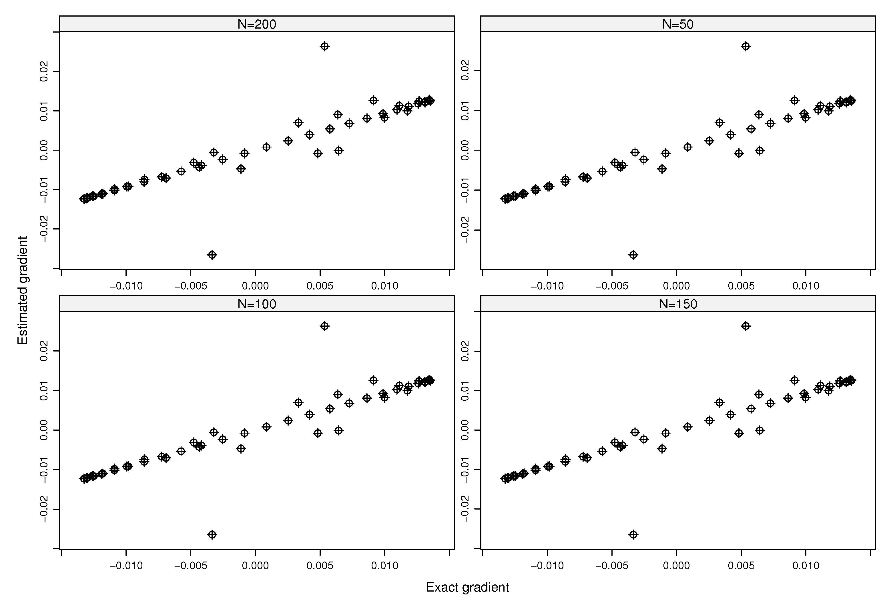
Figure 1 shows the comparisons between the estimated and the exact values of the formal gradient (i.e., ) for . Likewise, Figure 2Figure 3 depict the dependent gradient and its estimation. The estimates of both gradients are in line with the exact values using only (resp. ) model evaluations when and (resp. and or and ). Increasing the values of L and N gives the same quasi-perfect results for both the formal and dependent gradients (see Figure 3).
6. Conclusion
In this paper, we have proposed new, simple and generic approximations of the gradients of functions with non-independent input variables by means of independent, central and symmetric variables and a set of constraints. It comes out that the biases of our approximations for a wide class of functions, such as 2-smooth functions, do not suffer from the curse of dimensionality by properly choosing the set of independent, central and symmetric variables. For functions including only independent input variables, a theoretical comparison has shown that the upper-bounds of the bias of the formal gradient derived in this paper outperform the best known results.
For computing the dependent gradient of the function of interest, we have provided estimators of such a gradient by making use of evaluations of that function at randomized points. Such estimators reach the optimal (mean squared error) rates of convergence (i.e., ) for a wide class of functions. Numerical comparisons using a test case and simulations based on a PDE model with given auto-collaborations among the initial conditions have shown the efficiency of our approach, even when constraints are used. Our approach is then flexible thanks to L and the fact that the gradient can be computed for every value of the sample size N in general.
While the proposed estimators reach the parametric rate of convergence, note that the second-order moments of such estimators depend on . An attempt to reach a dimension-free rate of convergence requires working in rather than when . In next future, it is worth investigating the derivation of the optimal rates of convergence that are dimension-free or (at least) are linear with respect to d by considering constraints. Also, combining such a promising approach with a transformation of the original space might be helpful for reducing the number of model evaluations in higher dimensions.
Acknowledgments
We would like to thank the reviewers for their comments that have helped improving our manuscript.
Appendix A. Proof of Theorem 1
As , let and . Multiplying the Taylor expansion of about , that is,
by and the constant , and taking the sum over , we can see that the expectation becomes
Firstly, for a given and by independence, we can see that
iff ; for any with , which implies that . Thus, one obtains when , and the fact that ; and . At this point, by taking and setting and result in the approximation of of order because when , .
Secondly, for the constraints allow to eliminate some higher-order terms so as to reach the order . Using other constraints complete the proof, bearing in mind Equation (2).
Appendix B. Proof of Corollary 1
For ; and , consider . As , we can write
with the remainder term
Denote , and remark that . Using Theorem 1, we can see that the absolute value of the bias, that is,
is given by
using the expansion of the product between matrices.
Using the same reasoning and taking the Euclidean norm, we obtain
The results hold using .
Appendix C. Proof of Theorem 2
Firstly, remark that is given by
Since, the bias has been derived in previous Corollaries, we are going to treat the second-order moment.
Secondly, as implies that , we have Also, as , we then have
which leads to and
Thirdly, using (3), we can see that . Bearing in mind the definition of the Euclidean norm and the variance, the centered second-order moment, that is, is given by
bearing in mind the Hölder inequality. The results hold using , and the fact that when , and .
References
- Rosenblatt, M. Remarks on a Multivariate Transformation. Ann. Math. Statist. 1952, 23, 470–472. [Google Scholar]
- Nataf, A. Détermination des distributions dont les marges sont données. Comptes Rendus de l’Académie des Sciences 1962, 225, 42–43. [Google Scholar]
- Joe, H. Dependence Modeling with Copulas; Chapman & Hall/CRC, London, 2014.
- McNeil, A.J.; Frey, R.; Embrechts, P. Quantitative Risk Management; Princeton University Press, Princeton and Oxford, 2015.
- Navarro, J.; Ruiz, J.M.; Aguila, Y.D. Multivariate weighted distributions: a review and some extensions. Statistics 2006, 40, 51–64. [Google Scholar]
- Sklar, A. Fonctions de Repartition a n Dimensions et Leurs Marges. Publications de l’Institut Statistique de l’Universite de Paris 1959, 8, 229–231. [Google Scholar]
- Durante, F.; Ignazzi, C.; Jaworski, P. On the class of truncation invariant bivariate copulas under constraints. Journal of Mathematical Analysis and Applications 2022, 509, 125898. [Google Scholar]
- Skorohod, A.V. On a representation of random variables. Theory Probab. Appl 1976, 21, 645–648. [Google Scholar]
- Lamboni, M.; Kucherenko, S. Multivariate sensitivity analysis and derivative-based global sensitivity measures with dependent variables. Reliability Engineering & System Safety 2021, 212, 107519. [Google Scholar]
- Lamboni, M. Efficient dependency models: Simulating dependent random variables. Mathematics and Computers in Simulation 2022. [Google Scholar] [CrossRef]
- Lamboni, M. On exact distribution for multivariate weighted distributions and classification. Methodology and Computing in Applied Probability 2023, 25, 1–41. [Google Scholar]
- Lamboni, M. Measuring inputs-outputs association for time-dependent hazard models under safety objectives using kernels. International Journal for Uncertainty Quantification 2024, -, 1–17. [CrossRef]
- Kucherenko, S.; Klymenko, O.; Shah, N. Sobol’ indices for problems defined in non-rectangular domains. Reliability Engineering & System Safety 2017, 167, 218–231. [Google Scholar]
- Lamboni, M. On dependency models and dependent generalized sensitivity indices. arXiv preprint arXiv2104.12938 2021. [Google Scholar]
- Lamboni, M. Derivative Formulas and Gradient of Functions with Non-Independent Variables. Axioms 2023, 12. [Google Scholar] [CrossRef]
- Nemirovsky, A.; Yudin, D. Problem Complexity and Method Efficiency in Optimization; Wiley & Sons, New York, 1983; p. 404.
- Patelli, E.; Pradlwarter, H. Monte Carlo gradient estimation in high dimensions. International Journal for Numerical Methods in Engineering 2010, 81, 172–188. [Google Scholar]
- Agarwal, A.; Dekel, O.; Xiao, L. Optimal Algorithms for Online Convex Optimization with Multi-Point Bandit Feedback. Colt. Citeseer, 2010, pp. 28–40.
- Bach, F.; Perchet, V. Highly-Smooth Zero-th Order Online Optimization. 29th Annual Conference on Learning Theory; Feldman, V.; Rakhlin, A.; Shamir, O., Eds., 2016, Vol. 49, pp. 257–283.
- Akhavan, A.; Pontil, M.; Tsybakov, A.B. Exploiting higher order smoothness in derivative-free optimization and continuous bandits; Curran Associates Inc.: Red Hook, NY, USA, 2020; NIPS ’20. [Google Scholar]
- Sobol, I.M.; Kucherenko, S. Derivative based global sensitivity measures and the link with global sensitivity indices. Mathematics and Computers in Simulation 2009, 79, 3009–3017. [Google Scholar]
- Kucherenko, S.; Rodriguez-Fernandez, M.; Pantelides, C.; Shah, N. Monte Carlo evaluation of derivative-based global sensitivity measures. Reliability Engineering and System Safety 2009, 94, 1135–1148. [Google Scholar]
- Lamboni, M.; Iooss, B.; Popelin, A.L.; Gamboa, F. Derivative-based global sensitivity measures: General links with Sobol’ indices and numerical tests. Mathematics and Computers in Simulation 2013, 87, 45–54. [Google Scholar]
- Roustant, O.; Fruth, J.; Iooss, B.; Kuhnt, S. Crossed-derivative based sensitivity measures for interaction screening. Mathematics and Computers in Simulation 2014, 105, 105–118. [Google Scholar]
- Fruth, J.; Roustant, O.; Kuhnt, S. Total interaction index: A variance-based sensitivity index for second-order interaction screening. Journal of Statistical Planning and Inference 2014, 147, 212–223. [Google Scholar]
- Lamboni, M. Derivative-based generalized sensitivity indices and Sobol’ indices. Mathematics and Computers in Simulation 2020, 170, 236–256. [Google Scholar]
- Lamboni, M. Derivative-based integral equalities and inequality: A proxy-measure for sensitivity analysis. Mathematics and Computers in Simulation 2021, 179, 137–161. [Google Scholar]
- Lamboni, M. Weak derivative-based expansion of functions: ANOVA and some inequalities. Mathematics and Computers in Simulation 2022, 194, 691–718. [Google Scholar]
- Bobkov, S. Isoperimetric and Analytic Inequalities for Log-Concave Probability Measures. The Annals of Probability 1999, 27, 1903–1921. [Google Scholar]
- Roustant, O.; Barthe, F.; Iooss, B. Poincare inequalities on intervals - application to sensitivity analysis. Electron. J. Statist. 2017, 11, 3081–3119. [Google Scholar]
- Le Dimet, F.X.; Talagrand, O. Variational algorithms for analysis and assimilation of meteorological observations: theoretical aspects. Tellus A: Dynamic Meteorology and Oceanography 1986, 38, 97–110. [Google Scholar]
- Le Dimet, F.X.; Ngodock, H.E.; Luong, B.; Verron, J. Sensitivity analysis in variational data assimilation. Journal-Meteorological Society of Japan 1997, 75, 245–255. [Google Scholar]
- Cacuci, D.G. Sensitivity and uncertainty analysis - Theory; Chapman & Hall/CRC, 2005.
- Gunzburger, M.D. Perspectives in flow control and optimization; SIAM, Philadelphia, 2003.
- Borzi, A.; Schulz, V. Computational Optimization of Systems Governed by Partial Differential Equations; SIAM, Philadelphia, 2012.
- Ghanem, R.; Higdon, D.; Owhadi, H. Handbook of Uncertainty Quantification; Springer International Publishing, 2017.
- Guidotti, E. calculus: High-Dimensional Numerical and Symbolic Calculus in R. Journal of Statistical Software 2022, 104, 1–37. [Google Scholar]
- Ancell, B.; Hakim, G.J. Comparing Adjoint- and Ensemble-Sensitivity Analysis with Applications to Observation Targeting. Monthly Weather Review 2007, 135, 4117–4134. [Google Scholar]
- Pradlwarter, H. Relative importance of uncertain structural parameters. Part I: algorithm. Computational Mechanics 2007, 40, 627–635. [Google Scholar]
- Polyak, B.; Tsybakov, A. Optimal accuracy orders of stochastic approximation algorithms. Probl. Peredachi Inf. 1990, pp. 45–53.
- Zemanian, A. Distribution Theory and Transform Analysis: An Introduction to Generalized Functions, with Applications; Dover Books on Advanced Mathematics, Dover Publications, 1987.
- Strichartz, R. A Guide to Distribution Theory and Fourier Transforms; Studies in advanced mathematics, CRC Press, Boca, 1994.
- Lamboni, M. Kernel-based Measures of Association Between Inputs and Outputs Using ANOVA. Sankhya A 2024. [Google Scholar] [CrossRef]
- Gilbert, P.; Varadhan, R. R-package numDeriv: Accurate Numerical Derivatives; CRAN Repository, 2019.
- Soetaert et al., K. R-package deSolve: Solvers for Initial Value Problems of Differential Equations; CRAN Repository, 2022.
Figure 1.
Exact gradient versus estimated gradients using (∘) and (+) of the QoI by considering the inputs as independent (formal gradients).
Figure 1.
Exact gradient versus estimated gradients using (∘) and (+) of the QoI by considering the inputs as independent (formal gradients).
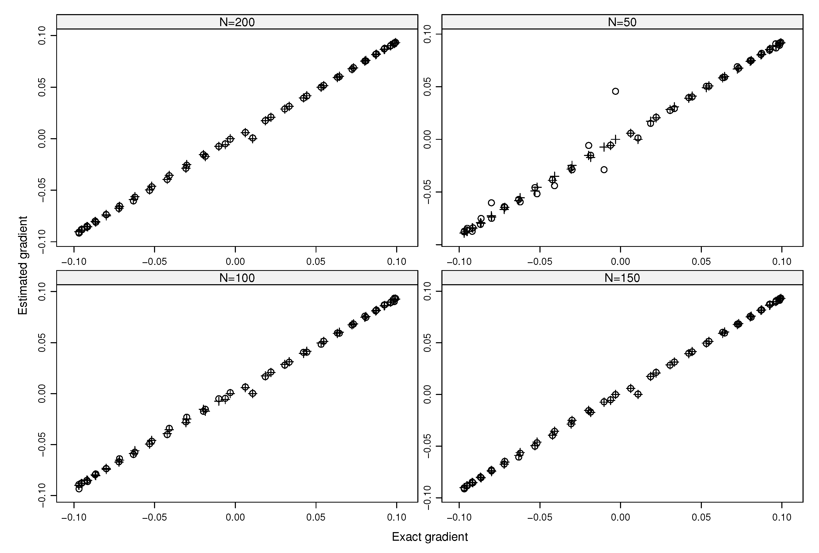
Figure 2.
Exact gradient versus estimated gradients using (∘) and (+) of the QoI by considering the auto-correlations anong the inputs (dependent gradients).
Figure 2.
Exact gradient versus estimated gradients using (∘) and (+) of the QoI by considering the auto-correlations anong the inputs (dependent gradients).
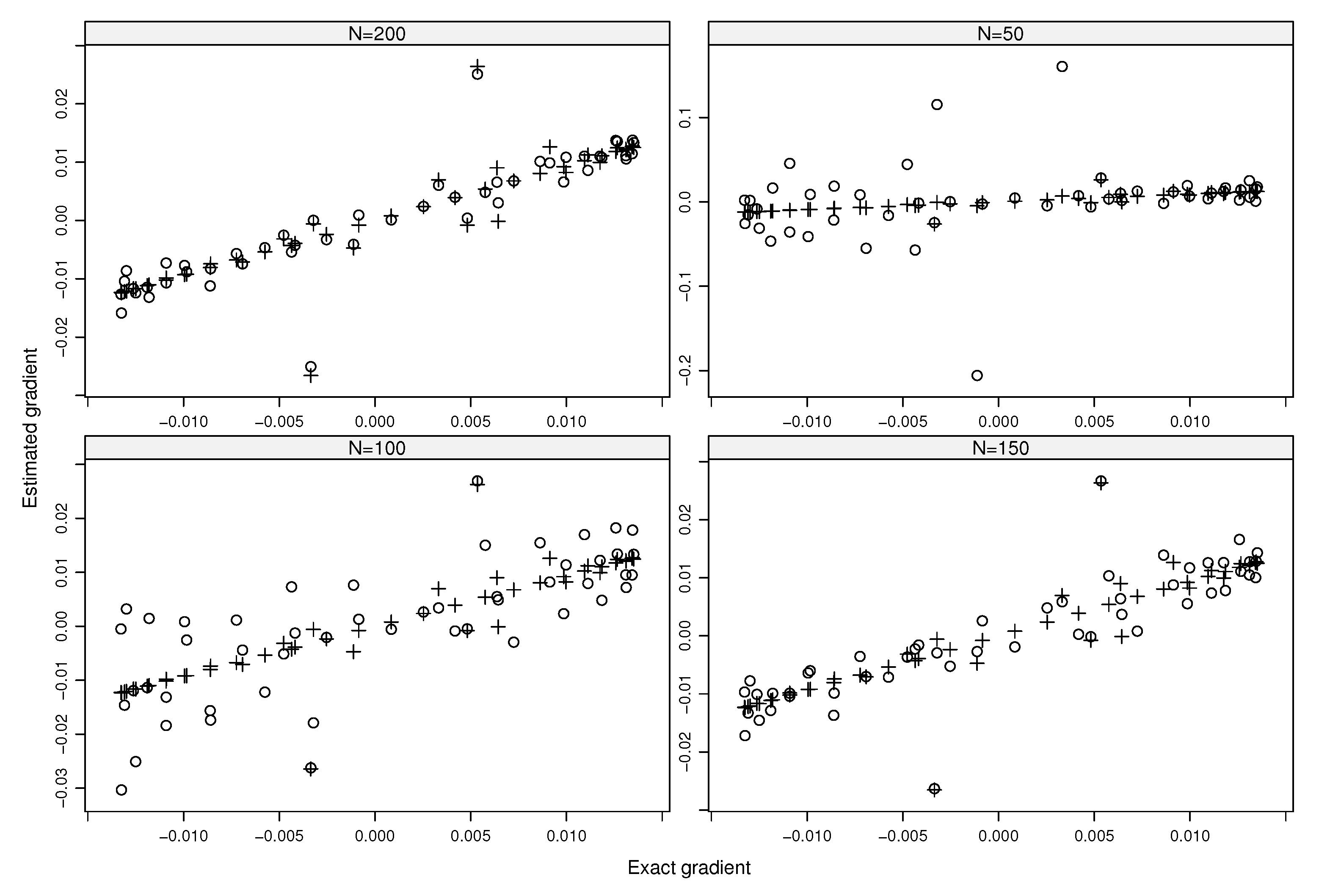
Figure 3.
Exact gradient versus estimated gradients using (∘) and (+) of the QoI by considering the auto-correlations anong the inputs (dependent gradients).
Figure 3.
Exact gradient versus estimated gradients using (∘) and (+) of the QoI by considering the auto-correlations anong the inputs (dependent gradients).

Disclaimer/Publisher’s Note: The statements, opinions and data contained in all publications are solely those of the individual author(s) and contributor(s) and not of MDPI and/or the editor(s). MDPI and/or the editor(s) disclaim responsibility for any injury to people or property resulting from any ideas, methods, instructions or products referred to in the content. |
© 2024 by the authors. Licensee MDPI, Basel, Switzerland. This article is an open access article distributed under the terms and conditions of the Creative Commons Attribution (CC BY) license (http://creativecommons.org/licenses/by/4.0/).
Copyright: This open access article is published under a Creative Commons CC BY 4.0 license, which permit the free download, distribution, and reuse, provided that the author and preprint are cited in any reuse.


