A Reformulation of the Lambert Conformal Conic Projection with Application to Bulgarian National Mapping

1. Introduction

The fundamental principles of conic conformal map projections were established by Johann Heinrich Lambert in 1772 [1]. In recognition of his contributions, these projections are known as Lambert conic conformal map projections. In the third part of his Beyträge zum Gebrauche der Mathematik und deren Anwendung (Contributions to the Usage of Mathematics and Its Application, 1772), titled Anmerkungen und Zusätze zur Entwerfung der Land- und Himmelscharten (Remarks and Additions to the Establishment of Terrestrial and Celestial Maps), Lambert describes the projection of spheres and spheroids onto a plane. Consequently, according to Frischauf (1905) [2], Deetz and Adams (1934) [3], Lapaine and Kuveždić (2007) [4], and others, Lambert may be regarded as the founder of general map projection theory. Whereas his predecessors investigated only individual projections, Lambert approached the problem of mapping a surface onto a plane from a broader perspective and formulated general mathematical conditions that such mappings must satisfy. The most important of these conditions concern the preservation of angles (conformality) and the preservation of area (equivalence). Although Lambert did not develop a complete theory of these mappings, he was the first to articulate these ideas in a clear and systematic manner.

In this paper, we focus on a conformal conic projection known as the Lambert conformal conic (LCC). For completeness, we derive the equations of this projection in Section 2. In doing so, we introduce a new variable, V, defined as the reciprocal of the commonly used quantity U, to simplify the notation in the resulting formulas. Special attention is given to distortion characteristics, enabling us to formulate, at the end of this section, the conditions that determine whether the projection has two, one, or no standard parallels.

The basic form of the LCC projection includes two parameters that influence the distribution of linear and areal distortions over the territory to which the projection is applied. In Section 3, we describe a criterion well known in the literature: the optimal LCC projection is obtained when the two parameters are chosen such that the local linear scale factors along the two boundary parallels are equal and the maximum local linear scale factor exceeds unity by the same amount that the minimum local linear scale factor falls below unity.

In Section 4, we apply this criterion to compute the projection parameters and determine the standard parallels for an optimal LCC projection for the territory of Bulgaria, which constitutes the principal objective of this paper.

2. Lambert Conformal Conic Projection

In normal conic projections, meridians are mapped as straight lines that intersect at angles proportional to the differences in their longitudes. Parallels are represented as arcs of concentric circles centered at the point where the meridians converge. To depict the region of interest on a plane, it is necessary to establish a relationship between the geodetic coordinates φ and λ on the ellipsoid or sphere and the corresponding planar coordinates. In conic projections, the planar coordinates are expressed using the polar angle δ and the polar radius ρ (Fig. 1).

Figure 1. Coordinate system in normal conic projections.

Figure 1. Coordinate system in normal conic projections.

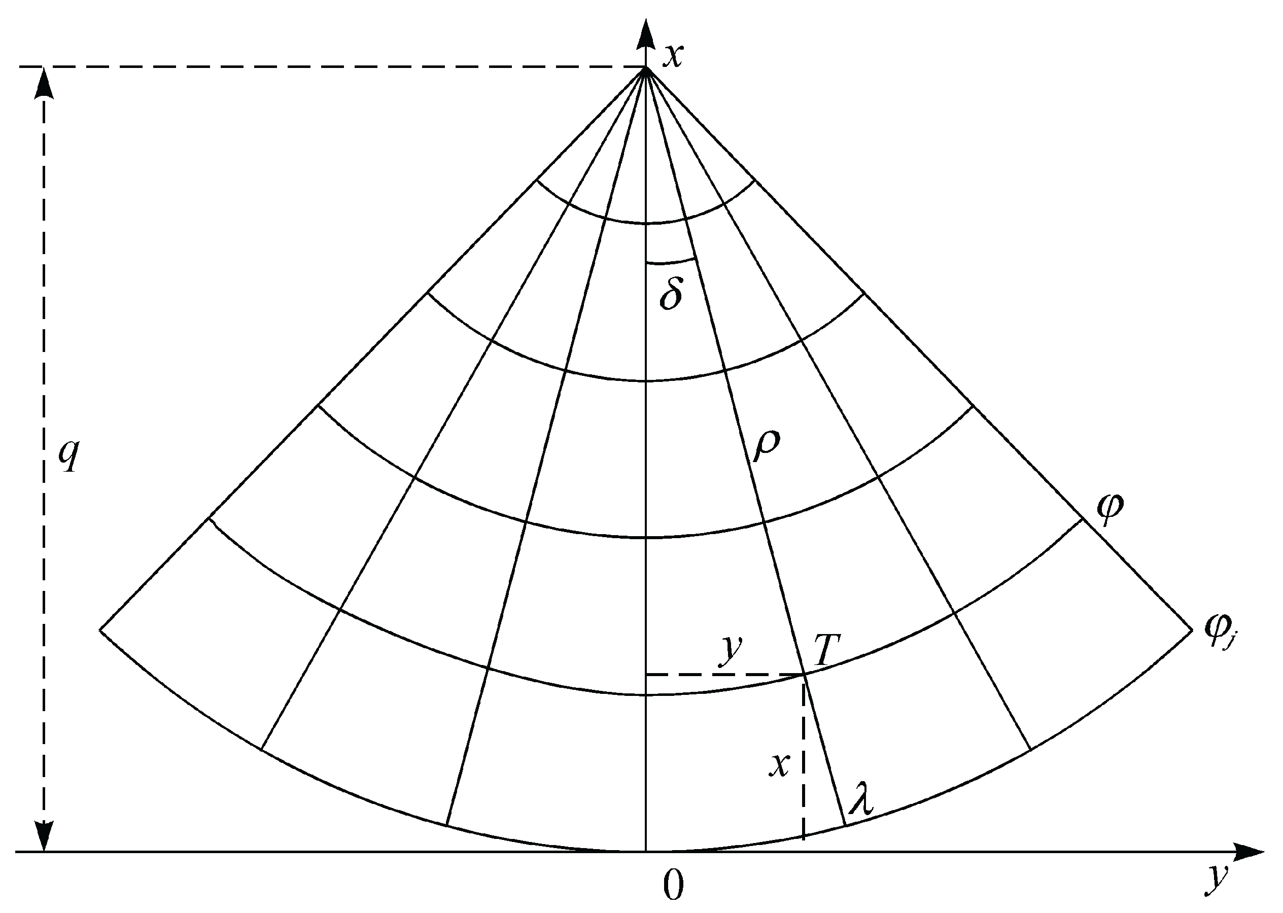
The general equations of normal conic projection in polar coordinates are defined as follows (Fig. 1):

$$\rho =\rho \left(\phi \right),$$

(1)

$$\delta =n\left(\lambda -{\lambda }_0\right),$$

(2)

where n is proportionality constant, $\lambda$ is longitude and ${\lambda }_0$ is longitude of the central meridian of the projected area.

The form of the function $\rho =\rho \left(\phi \right)$ determines whether the projection is conformal, equivalent, or equidistant. The relationship between polar and rectangular coordinates is:

$$x=q-\rho \cos \delta ,$$

(3)

$$y=\rho \sin \delta ,$$

(4)

where q is the radius of the parallel with the smallest latitude in the projected area (Fig. 1). The x-axis of the rectangular coordinate system coincides with the polar axis, and the origin is located at the intersection of the southernmost parallel and the central meridian in the projection plane (Fig. 1).

Formulas for the linear scale factors along meridians and parallels are well established in the literature [5,6]. The local linear scale factor along a meridian is $h={\displaystyle \frac{\sqrt{E}}{M}}$ and the local linear scale factor along a parallel is $k={\displaystyle \frac{\sqrt{G}}{r}}$. In these expressions, E and G are the first fundamental quantities of Gauss; M is the meridional radius of curvature; N is the radius of curvature in the prime vertical; and r is the radius of the parallel, computed using the expression:

$$r=r\left(\phi \right)=N\cos \phi .$$

(5)

Required partial derivations are:

$${\displaystyle \frac{\partial x}{\partial \phi }}={\displaystyle \frac{d\rho }{d\phi }}\cos \delta ,{\displaystyle \frac{\partial y}{\partial \phi }}={\displaystyle \frac{d\rho }{d\phi }}\sin \delta ,$$

(6)

$${\displaystyle \frac{\partial x}{\partial \lambda }}=n\rho \sin \delta ,{\displaystyle \frac{\partial y}{\partial \lambda }}=n\rho \cos \delta .$$

(7)

Thus

$$E={\left({\displaystyle \frac{d\rho }{d\phi }}\right)}^2, G=n^2{\rho }^2$$

(8)

and finally

$$h=-{\displaystyle \frac{d\rho }{Md\phi }},k={\displaystyle \frac{n\rho }{r}}.$$

(9)

Due to conformality of the Lambert conic projection

$$-{\displaystyle \frac{d\rho }{Md\phi }}={\displaystyle \frac{n\rho }{r}}.$$

(10)

from which the function $\rho =\rho \left(\phi \right)$ can be determined. If the expressions for r, M and N are substituted into the above relation, it becomes

$$-{\displaystyle \frac{d\rho }{\rho }}=n{\displaystyle \frac{M}{N}} {\displaystyle \frac{d\phi }{\cos \phi }}=n{\displaystyle \frac{1-e^2}{1-e^2{\sin }^2\phi }} {\displaystyle \frac{d\phi }{\cos \phi }},$$

(11)

where e is the eccentricity of the ellipsoid. The integral of the term multiplying n on the right-hand side of (11) corresponds to the isometric latitude, which appears in all conformal mappings of the ellipsoid. After integration, we obtain

$$\ln \rho =-n\ln \tan \left({\displaystyle \frac{\pi }{4}}+{\displaystyle \frac{\phi }{2}}\right)+ne\ln \tan \left({\displaystyle \frac{\pi }{4}}+{\displaystyle \frac{\psi }{2}}\right)+\ln F,$$

(12)

where F is the integration constant, and $\psi$ is the function of latitude determined with the expression

$$\mathrm{s}\mathrm{i}\mathrm{n} \psi =e\sin \phi .$$

(13)

The previous equation can be written in a simpler form, as

$$\rho \left(\phi \right)={\displaystyle \frac{F}{U^n\left(\phi \right)}}=F{V}^n\left(\phi \right) ,$$

(14)

where

$$V\left(\phi \right)={\displaystyle \frac{1}{U\left(\phi \right)}}={\displaystyle \frac{{\tan }^e\left(\frac{\pi }{4}+\frac{\psi }{2}\right)}{\tan \left(\frac{\pi }{4}+\frac{\phi }{2}\right)}}=\tan \left({\displaystyle \frac{\pi }{4}}-{\displaystyle \frac{\phi }{2}}\right){\tan }^e\left({\displaystyle \frac{\pi }{4}}+{\displaystyle \frac{\psi }{2}}\right).$$

(15)

In the map projection literature, the designation U is commonly used. For convenience, we introduce its reciprocal, V, as defined in equation (15), to simplify the notation in subsequent formulas. Accordingly, the equations for conformal conic projections in the normal aspect are given by:

$$\delta \left(\lambda \right)= n\left(\lambda -{\lambda }_0\right),\rho \left(\phi \right) =F V^n\left(\phi \right),$$

(16)

$$V \left(\phi \right)=\tan \left({\displaystyle \frac{\pi }{4}}-{\displaystyle \frac{\phi }{2}}\right){\tan }^e\left({\displaystyle \frac{\pi }{4}}+{\displaystyle \frac{\psi }{2}}\right), \mathrm{s}\mathrm{i}\mathrm{n} \psi =e\sin \phi$$

(17)

$$x=q-\rho \cos \delta ,y=\rho \sin \delta ,$$

(18)

$$h=k={\displaystyle \frac{n\rho }{r}} , p=k^2 , \omega =0.$$

(19)

In the preceding formulae, $\rho$ denotes the local area scale factor, and $\omega$ represents the maximum angular distortion. These formulae involve two constants, $n$ and $F$, which can be determined under various conditions. Together, they define the Lambert conformal conic projection, hereafter referred to as LCC.

For $\phi =0$, we have $V\left(0\right)=1$ and $\rho \left(0\right)=F$; thus, $F$ corresponds to the radius of the equator’s image in the projection plane.

We now examine the distribution of the local linear scale factor, $k= {\displaystyle \frac{n\rho }{r}}$ in greater detail, beginning with the determination of its extreme values.

$$k=k\left(\phi \right)={\displaystyle \frac{n\rho \left(\phi \right)}{r\left(\phi \right)}},\phi \in \left(-\pi /2,\pi /2\right).$$

(20)

From the condition

$${\displaystyle \frac{dk}{d\phi }}=n{\displaystyle \frac{M\rho }{r^2}}\left(\sin \phi -n\right)=0$$

(21)

it follows that the stationary point ${\phi }_0$ satisfies

$$n=\sin {\phi }_0.$$

(22)

Because a stationary point may correspond to either a minimum or a maximum, we now determine which case applies. To this end, we compute the second derivative of the function $k=k\left(\phi \right)$. At the stationary point, we obtain

$${\displaystyle \frac{d^{2}k}{d{\phi }^2}}=n{\displaystyle \frac{\rho \left({\phi }_0\right)M\left({\phi }_0\right)}{r\left({\phi }_0\right)N\left({\phi }_0\right)}}>0,$$

(23)

which indicates that the stationary point is a minimum. The derivation up to this point is well known in the literature on map projections [3,6,7,8,9,10]. We now extend this result. In particular, we ask how many standard parallels the LCC projection can possess. To answer this question, we examine the corresponding condition: for a parallel to be standard, it is necessary that at every point on it,

$$h\left(\phi \right)=k\left(\phi \right)=1.$$

(24)

Since in conformal projections $h\left(\phi \right)=k\left(\phi \right)$ at every point, and since in the LCC projection the local linear scale factors depend only on the geodetic latitude $\phi$, it is sufficient to examine the condition

$$k\left(\phi \right)=1.$$

(25)

Using equation (20), we may first write

$${\displaystyle \frac{n\rho \left(\phi \right)}{r\left(\phi \right)}}=1,$$

(26)

and then, by applying equations (16) and (17),

$${\displaystyle \frac{nF{V}^n\left(\phi \right)}{r\left(\phi \right)}}=1,$$

(27)

From this, it follows that

$$F={\displaystyle \frac{r\left(\phi \right)}{n{V}^n\left(\phi \right)}}.$$

(28)

Now, if we wish the parallel corresponding to the geodetic latitude ${\phi }_0$ from relation (22) to be standard − i.e., for the local linear scale factor to equal 1 along that parallel − then we must choose

$$F{=F}_0={\displaystyle \frac{r\left({\phi }_0\right)}{n{V}^n\left({\phi }_0\right)}}.$$

(29)

In this case, the local linear scale factor attains its minimum value of 1 at ${\phi }_0$, and therefore the scale factor along all other parallels is greater than 1 (blue curve in Fig. 2). This corresponds to the situation with a single standard parallel.

Figure 2. The local linear scale factor $k=k\left(\phi \right)$ of the LCC projection as a function of the parameter F. Blue: one standard parallel; red: two standard parallels; green: no standard parallels.

Figure 2. The local linear scale factor $k=k\left(\phi \right)$ of the LCC projection as a function of the parameter F. Blue: one standard parallel; red: two standard parallels; green: no standard parallels.

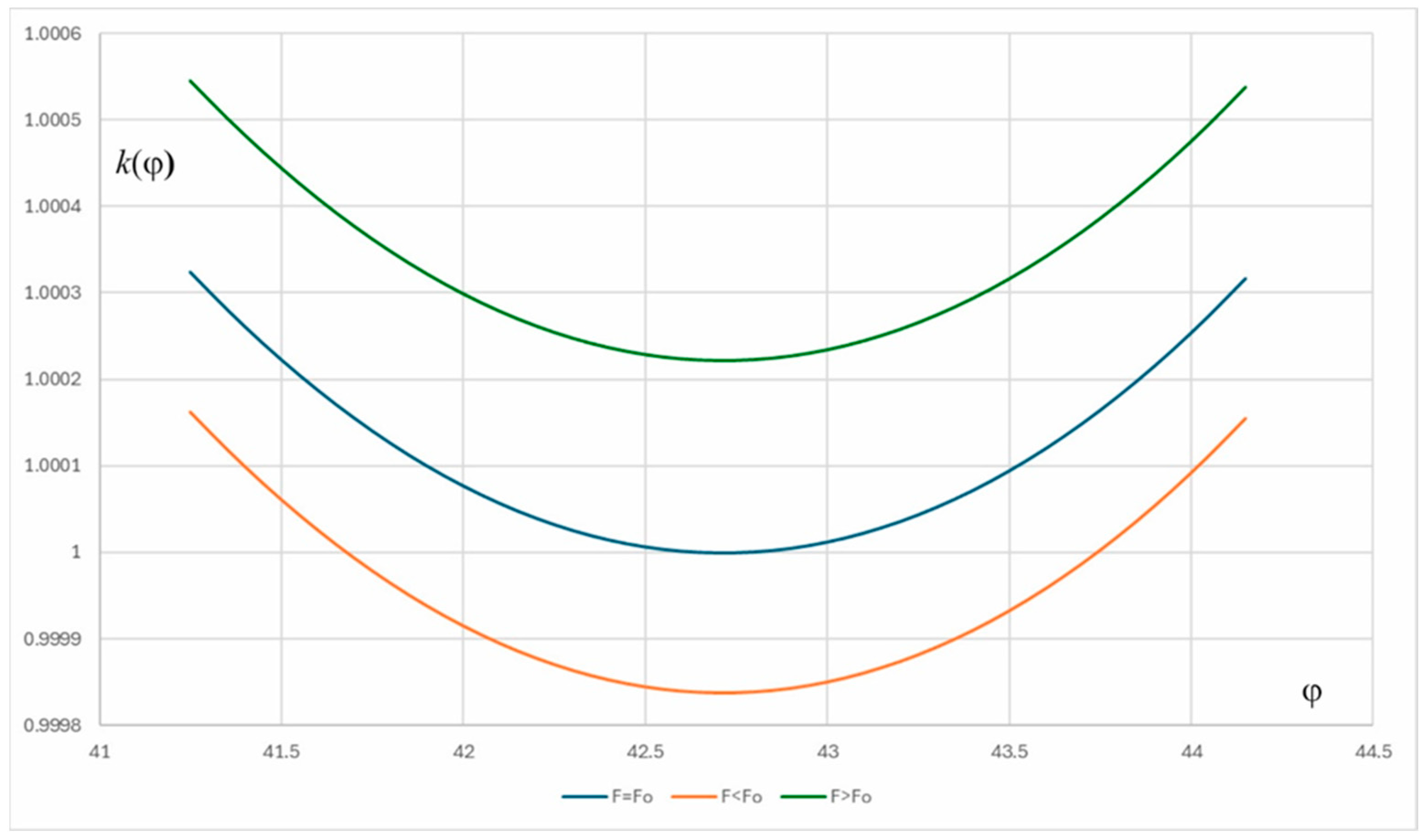
If we choose $F{>F}_0$, so that $k\left(\phi \right)>1$, then the projection will have no standard parallels (green curve in Fig. 2). Conversely, if we choose $F{<F}_0$, then there will exist two distinct latitudes ${\phi }_1$ and ${\phi }_2$ such that $k\left({\phi }_1\right)=k\left({\phi }_2\right)=1$. In this case, the projection possesses two standard parallels (red curve in Fig. 2). Furthermore, if we choose $F{=F}_0$, only one standard parallel exists.

3. The Optimal LCC Projection

In principle, every map projection can be considered optimal in some sense. However, map projection theory offers a variety of criteria for defining what “optimal” means [3,6,7,8,9,10,11,12,13,14,15,16,17,18,19,20,21,22,23,24,25,26].

Because any projection may be regarded as “optimal” depending on the chosen criterion, it is important to specify what “optimal projection” means in our context. Since we are considering conformal projections − those free of angular distortion and with area distortion equal to the square of the linear distortion − it suffices to formulate a criterion based solely on linear distortions.

If there is no particular reason for the local linear scale factors along the southernmost and northernmost parallels of the mapped region to differ, it is natural to require them to be equal. Denote the geodetic latitudes of these two boundary parallels by ${\phi }_S$ and ${\phi }_N$, respectively. This requirement can be expressed mathematically as:

$$k\left({\phi }_S\right)=k\left({\phi }_N\right).$$

(30)

If there is no particular reason for the minimum and maximum values of linear distortion to differ in absolute magnitude, it is natural to require that they be equal. This condition can be expressed mathematically as

$$k\left({\phi }_S\right)-1=1-k\left({\phi }_0\right)=k\left({\phi }_N\right)-1,$$

(31)

where ${\phi }_0$ is the geodetic latitude of the parallel at which the local linear scale factor attains its minimum. Accordingly, we propose the following criterion for selecting the optimal LCC projection for an area bounded by the parallels ${\phi }_S$ and ${\phi }_N$.

The optimal LCC projection is the one in which the parameters $n$ and $F$ from equation (16) are chosen such that the local linear scale factors along the two boundary parallels are equal, and the maximum local linear scale factor exceeds 1 by the same amount that the minimum local linear scale factor falls below 1.

This criterion is well established in the literature on map projections [3,6,7,9,10,15,16,18,22,27]; here, we presented a clearer formulation of it. For convenience, let us introduce the notation

$$r_s=r\left({\phi }_S\right), r_N=r\left({\phi }_N\right), V_S=V\left({\phi }_S\right) ,V_N=V\left({\phi }_N\right)$$

(32)

$${\rho }_S=F{V}_S^n, {\rho }_N=F{V}_N^n{k}_S=k\left({\phi }_S\right), k_N=k\left({\phi }_N\right),$$

(33)

If the scale factors along the two boundary parallels are equal (30), the expression for the constant n becomes:

$$n={\displaystyle \frac{\ln r_N-\ln r_S}{\ln V_N-\ln V_S}}={\displaystyle \frac{\ln \left(r_N/r_S\right)}{\ln \left(V_N/V_S\right)}}.$$

(34)

The expression for the constant $F$ follows from the second requirement − that the maximum local linear scale factor exceeds 1 by the same amount that the minimum local linear scale factor falls below 1:

$$F={\displaystyle \frac{2}{n\left(V_N^n/r_N+V_0^n/r_0\right)}}={\displaystyle \frac{2}{n\left(V_S^n/r_S+V_0^n/r_0\right)}},$$

(35)

where

$$V_0=V\left({\phi }_0\right) ,r_0=r\left({\phi }_0\right).$$

(36)

Starting from the given geodetic latitudes ${\phi }_S$ and ${\phi }_N$, we thus determine the projection constants $n$ and $F$. Once these parameters are known, the geodetic latitudes ${\phi }_1$ and ${\phi }_2$ of the standard parallels (where the scale factor equals 1) can be found by solving the transcendental equation:

$$nF{V}^n\left(\phi \right)=r\left(\phi \right),$$

(37)

which may be solved using an appropriate iterative method.

Finally, we examine a rule − reported by several authors, including Hinks, Kavrayskiy, Deetz and Adams − for the approximate determination of the positions of the standard parallels. The rule is given by

$${\phi }_1={\phi }_S+{\displaystyle \frac{{\phi }_N-{\phi }_S}{K}},{\phi }_2={\phi }_N-{\displaystyle \frac{{\phi }_N-{\phi }_S}{K}},$$

(38)

where $K$ = 3,4,5,6, or 7, depending on the shape of the mapped region (e.g., circular, square, etc.) [7].

According to Hinks, it is generally sufficient to place the standard parallels at approximately one-seventh of the total latitudinal extent inward from the bounding parallels [11].

Deetz and Adams [3] state that, for an approximately equal distribution of scale error, the standard parallels should be selected at one-sixth and five-sixths of the length of the portion of the central meridian being represented.

In 1962, the projection used for the International Map of the World (IMW) at a scale of 1:1,000,000 was changed from a modified Polyconic to the LCC projection for latitudes between 84° N and 80° S. A polar stereographic projection is used for the remaining areas. Each sheet covers approximately 6° of longitude by 4° of latitude. Within each 4° latitudinal zone, the standard parallels are placed at one-sixth and five-sixths of the latitude span. The reference ellipsoid adopted was the International ellipsoid. This specification was subsequently used by the United States Geological Survey (USGS) in producing several maps for the IMW series.

The USGS also employs the LCC projection for topographic purposes in the middle latitudes for the 1:1,000,000-scale geologic series of the Moon, as well as for selected maps of Mercury, Mars, and the satellites of Jupiter [5].

Using relation (38), the parameter $K$ can be expressed as follows:

$$K={\displaystyle \frac{{\phi }_N-{\phi }_S}{{\phi }_1-{\phi }_S}} \mathrm{or} K={\displaystyle \frac{{\phi }_N-{\phi }_S}{{\phi }_N-{\phi }_2}}.$$

(39)

For a sphere rather than an ellipsoid, all of the above formulas simplify, as one simply sets $e=0$.

4. The Optimal LCC Projection for the Territory of Bulgaria

The LCC projection has become a standard choice for official cartographic products worldwide, rivaled in prominence only by the Transverse Mercator projection [28]. Its significance is illustrated, for instance, by its adoption in Croatia, as outlined in the Decree on Establishing New Official Geodetic Datums and Planar Map Projections of the Republic of Croatia. On 4 August 2004, the Government of the Republic of Croatia established a coordinate reference system based on a normal LCC projection with standard parallels at 43°05′ and 45°55′ north for use in large-scale official mapping. The decision was motivated by the projection’s low linear distortions, its favorable preservation of areal and shape characteristics, and its broad applicability. The Croatian implementation of the LCC projection is based on the GRS80 ellipsoid. In accordance with ISO 19111 [29], the official abbreviation assigned to this projection system is HTRS96/LCC [30,31].

The aforementioned standard parallels were determined for the terrestrial portion of the Republic of Croatia. Rajaković and Lapaine examined the determination of optimal standard parallels for the entire national territory, which includes not only the mainland but also a section of the Adriatic Sea [27]. Based on their analysis, they proposed the standard parallels 42°20′ and 45°50′ north.

The Lambert Conformal Conic (LCC) projection has been employed in Bulgaria across all historically established and currently operational coordinate systems. Its configuration has varied, using either one or two standard parallels, along with differing parameter values, central meridians, and reference parallels. In the 1970 Coordinate System, the territory of Bulgaria was divided into four zones, each defined by an LCC projection with a single standard parallel. In the BGS 2000 and BGS 2005 coordinate systems, the projection is defined using two standard parallels, with the latter system primarily applied for cadastral purposes.

The use of this projection is determined by Bulgaria’s geographic location in the mid-latitudes and by the country’s predominantly east-west orientation along the parallels. Owing to these characteristics, the LCC projection has historically been regarded as the most appropriate choice for supporting national economic activities and land administration.

4.1. Bulgarian Geodetic System 2000

The Bulgarian Geodetic System 2000 (BGS2000) was officially introduced in 2002 [32]. Its specifications are detailed in an instruction issued by the Directorate Geodesy and Cartography of the Ministry of Regional Development and Public Works [33]. The LCC projection used in BGS2000 is defined by the following parameters:

The GRS80 ellipsoid is given by

a = 6378137 m, f = 1/298.257 222 101, e² = 6.69438002290×10^-3

φ_S = 41°15'; φ_N = 44°10'; φ_{1 =} 41°51'11.2153"; φ₂ = 43°28'35.8786" [33].

The method used to determine the standard parallels is not documented.

4.2. Bulgarian Geodetic System 2005

The Bulgarian Geodetic System 2005 (BGS2005) was introduced in 2012 [34,35]. It is employed for geodetic computations throughout the country and serves as the principal coordinate system for cartographic applications. The LCC projection in BGS2005 is defined by the following parameters:

The GRS80 ellipsoid is specified by

a = 6378137 m, f = 1/298.257 222 101, e² = 6.69438002290×10^-3

φ₁ = 42°00'00", φ₂ = 43°20'00", φ₀ = 42°40'04.35246" [34].

The geodetic latitudes of the southernmost φ_S and northernmost φ_N parallels are not explicitly defined. In the official Instruction [34], φ₀ is identified as the central parallel. However, the formulas provided in the Instruction show that φ₀ is in fact the geodetic latitude of the parallel along which the local linear scale factor n attains its minimum value. It would be more accurate to state that this latitude only approximately corresponds to the central parallel. The method used to determine the standard parallels is not documented.

4.3. Proposal by Bandrova and Gyurov

Bandrova and Gyurov define the optimal projection as the one in which the distortions at the mid-latitude and at the endpoints differ the least − that is, they are closest in magnitude [36]. They concluded that the most appropriate choice of standard parallels follows the 1/6 rule; however, in Table 7 of their article, they present standard parallels derived according to the 1/5 rule.

4.4. New Proposal

In contrast to the criterion proposed by Bandrova and Gyurov [36], the present study defines the optimal projection as the one for which the distortions at the midpoint latitude and at the endpoint latitudes do not differ in absolute value (Table 1). Applying this criterion to determine the optimal LCC projection for Bulgaria, using the GRS80 ellipsoid and the formulas presented in this article, and adopting the southernmost and northernmost parallels as follows:

φ_S = 41°14', φ_N = 44°13'

(40)

according to the Statistical Yearbook 2024 [37], which cites the Geodesy, Cartography and Cadastre Agency of the Ministry of Regional Development and Public Works as its data source, and

φ_S = 41°14'05", φ_N = 44°12'45"

(41)

according to Wikipedia [38], we obtained the following values:

${\phi }_S$	${\phi }_N$	${\phi }_1$	${\phi }_2$	${\phi }_0$	n	K
41°14'	44°13'	41°40'23.16"	43°46'58.08"	42°43'51.84"	0.67856	6.88 6.78
41°14'05"	44°12'45"	41°40'25.32"	43°46'46.20"	42°43'46.76"	0.67854	6.88 6.78

5. Conclusion

The Lambert Conformal Conic (LCC) projection was examined in detail in this study. The projection equations were derived, and instead of the commonly used notation U, a new notation V − defined as the reciprocal of U − was introduced to simplify the expression of the formulas. Particular attention was given to the analysis of distortions, which made it possible to formulate conditions governing the number of standard parallels, whether two, one, or none.

The equations of the LCC projection contain two parameters that determine the spatial distribution of length and area distortions over the territory to which the projection is applied. In this paper, we develop a criterion according to which the optimal LCC projection is defined as one in which these two parameters are selected such that the local linear scale factors along the boundary parallels are equal, and the maximum local linear scale factor exceeds 1 by the same amount that the minimum local linear scale factor falls below 1. We applied this criterion to compute the projection parameters and to determine the standard parallels for the optimal LCC projection for the territory of Bulgaria, which constitutes the primary objective of this study.

Table 1 shows that the local linear scale factors are nearly identical across all examined methods for selecting standard parallels. If we adopt the criterion that defines the optimal projection as the one in which the distortions at the midpoint latitude and at the endpoint latitudes do not differ in absolute value, then the optimal LCC projection for Bulgaria is the one whose standard parallels are

φ₁=41°40', φ₂=43°47'.

(42)

The maximum value of the local linear scale factor at the endpoint parallels is 1.00016824, while the minimum value is 0.99983176. For practical purposes, these values can be rounded to 1.0002 and 0.9998, respectively.

The average value of the parameter K was calculated as 6.92, which is approximately 7 and aligns with the general recommendation of Hinks [11]. Accordingly, the distance between the standard parallels and the extreme parallels corresponds to roughly one-seventh of the width of the 3° latitude band defined by the northernmost and southernmost parallels of Bulgaria.

References

- Lambert, J. H. Beyträge zum Gebrauche der Mathematik und deren Anwendung, Dritter Theil, im Verlag der Buchhandlung der Realschule, Berlin. Translated in English with an introduction by W. R. Tobler: Notes and Comments on the Composition of Terrestrial and Celestial Maps. In Michigan Geographical Publication No. 8, Department of Geography, University of Michigan; Ann Arbor, 1972. [Google Scholar]
- Frischauf, J. Die Abbildungslehre und deren Anwendung auf Kartographie und Geodäsie; Druck und Verlag von B. G. Teubner: Leipzig, 1905. [Google Scholar]
- Deetz, C. H.; Adams, O. S. Elements of Map Projection with Application to Map and Chart Construction. U. S. Coast and Geodetic Survey Special Publication 68, Washington, 1934.
- Lapaine, M.; Kuveždić, A. On the Development of Map Projections. Cartography and Geoinformation Special issue. 2007, pp. 110–147. Available online: https://hrcak.srce.hr/clanak/20113 (accessed on 19 December 2025).
- Snyder, J. P. Map Projections − A Working Manual, U.S. Geological Survey Professional Paper 1395. 1987. [Google Scholar]
- Bugaevskiy, L. M.; Snyder, J. P. Map Projections – A Reference Manual; Taylor & Francis: London, 1995. [Google Scholar]
- Kavrayskiy, V. V. Selected Works, Volume II, Mathematical Cartography, Issue 2, Conic and Cylindrical Projections and Their Applications. Published by the Office of the Chief of the Hydrographic Service of the VMF. 1959. [Google Scholar]
- Maling, D. H. Coordinate Systems and Map Projections; George Philip and Son Limited: London, 1973. [Google Scholar]
- Solov'ev, M. D. Map Projections; Publisher GUGK pri SNK SSSR: Moscow, 1946. [Google Scholar]
- Vitkovskiy, V. V. Cartography; Theory of map projections: St. Petersburg, 1907. [Google Scholar]
- Hinks, A. R. Map Projections; Cambridge University Press: Cambridge, 1912. [Google Scholar]
- Tsinger, N. Ya. O naivygodneyshikh vidakh konicheskikh proyektsiy Akademiya Nauk [St. Petersburg]. Izvestiya, series 6 1916, v. 10(no. 17), 1693. [Google Scholar]
- Chebyshev, P. L. On the Construction of Geographical Maps. St. Petersburg, Imperial Academy of Sciences, Physics and Mathematics Class, Bulletin, vol. 14, pp. 257-261. 1856. Reprinted in Works of P. L. Chebyshev: New York, Chelsea Pub. Co., 1962, vol. 1.
- Airy, G. B. Explanation of a projection by balance of errors for maps applying to a very large extent of the Earth's surface, and comparison of this projection with other projections. Philosophical Magazine and Journal of Science 1861, 22, 409–421. [Google Scholar] [CrossRef]
- Tissot, N. A. Memoir on the representation of surfaces and the projections of geographical maps; Gauthier Villars: Paris, 1881. [Google Scholar]
- Tissot, N. A. The network designs of geographical maps, Stuttgart, German edition by Ernst Hammer; 1887. [Google Scholar]
- Jordan, W. The mean distortion error. Journal of Surveying 1896, XXV, 249–252. [Google Scholar]
- Kavrayskiy, V. V. Selected Works, Volume II, Mathematical Cartography, Issue 1, General Theory of Cartographic Projects; Published by the Office of the Chief of the Hydrographic Service VMF, 1958. [Google Scholar]
- Meshcheryakov, I. A. Theoretical Foundations of Mathematical Cartography; Nedra Publishing House: Moscow, 1968. [Google Scholar]
- Milnor, J. A Problem in Cartography. The American Mathematical Monthly 1969, 76(10), 1101–1112. [Google Scholar] [CrossRef]
- Frančula, N. The most advantageous map projections in atlas cartography. dissertation, Faculty of Agriculture of the Rheinische Friedrich-Wilhelms University of Bonn, 1971. [Google Scholar]
- Canters, F. Small-scale Map Projection Design; Taylor & Francis: London and New York, 2002. [Google Scholar]
- Tutić, D. Optimal Conformal Polynomial Projections for Croatia According to the Airy/Jordan Criterion. Cartography and Geoinformation. Vol. 8, Nr. 11, pp. 48–67, 2009. https://hrcak.srce.hr/clanak/62104 (accessed on 22. 11. 2025).
- Šavrič, B.; Jenny, B. Automating the selection of standard parallels for conic map projections. Computers & Geosciences 2016, Vol. 90, Part A, 202–212. [Google Scholar] [CrossRef]
- Nestorov, I.; Kilibarda, M.; Protić, D. The optimal conformal projection for Pan-European mapping. Geodetski vestnik 2020, 64(2), 214–226. [Google Scholar] [CrossRef]
- Novikova, E. Best Map Projections. Springer Cham, 2025. [CrossRef]
- Rajaković, M.; Lapaine, M. The Best Conic Conformal Map Projection for the Territory of Croatia. Cartography and Geoinformation 2010, Vol. 9(Nr. 14), 24–44. Available online: https://hrcak.srce.hr/clanak/97209 (accessed on 24 November 2025).
- Snyder, J. P. Flattening the Earth; The University of Chicago Press: Chicago and London, 1993. [Google Scholar]
- ISO 19111:2019; Geographic information - Referencing by coordinates. Publisher: ISO, Geneva, Switzerland, 2019, https://www.iso.org/standard/74039.html (accessed on 20. 12. 2025).
- Lapaine, M. 20 years of new official map projections in Croatia. Geodetski list 2024, No. 1, 31–44. [Google Scholar]
- Lapaine, M.; Frančula, N. Map Projections with Reference to Their Applicationi in Croatia. Cartography and Geoinformation 2024, Vol. 23(No. 41), 22–51. [Google Scholar]
- RBMS. Decree No. 140 of the Council of Ministers of 4 June 2001 on the determination of the Bulgarian Geodetic System 2000, Promulgated, State Gazette, issue 54 of 2001, 2001.
- MRRB. Instruction for the implementation of the Decree of the Council of Ministers of the Republic of Bulgaria No. 140 of 04.06.2001 on the definition of the Bulgarian Geodetic System 2000 (BGS 2000), Ministry of Regional Development and Public Works, Directorate “Geodesy and Cartography”, Sofia, 2001.
- MRRB. Instruction No. RD-02-20-12 of August 3, 2012 for conversion of the existing geodetic and cartographic materials and data into the "Bulgarian Geodetic System 2005". Effective from 17.08.2012. Issued by the Ministry of Regional Development and Public Works, Sofia, 2012.
- MRRB. Ordinance No. RD-02-20-5 of December 15, 2016 on the content, creation and maintenance of the cadastral map and cadastral registers. Effective from 13.01.2017. Issued by the Ministry of Regional Development and Public Works, Sofia, 2016.
- Standard Parallels Choice for Lambert Conformal Conic Projection for Bulgaria − BGS2005, Proceedings, 9th International Conference on Cartography and GIS, Nessebar, Bulgaria, ISSN: 1314-0604, Eds: Bandrova T., Konečný M., Marinova S., pp. 96−105, 2024, https://shorturl.at/Ta5S9 (accessed on 24. 11. 2025).
- NSI. Statistical Yearbook 2024, Republic of Bulgaria, National Statistical Institute, 2025. Available online: https://www.nsi.bg/en/publications/statistical-yearbook-2024-9095 (accessed on 24 November 2025).
- Wikipedia. List of extreme points of Bulgaria, 2025. Available online: https://en.wikipedia.org/wiki/List_of_extreme_points_of_Bulgaria (accessed on 24 November 2025).