
Submitted:
31 December 2025
Posted:
01 January 2026
You are already at the latest version
Abstract
Development of AI-driven automated driving functions requires vast amounts of diverse, high-quality data to ensure road safety and reliability. However, manual collection of real-world data and creation of 3D environments is costly, time-consuming, and hard to scale. Most automatic environment generation methods still rely heavily on manual effort, and only a few are tailored for Advanced Driver Assistance Systems (ADAS) and Automated Driving (AD) training and validation. We propose an automated generative framework that learns real-world features to reconstruct realistic 3D environments from a road definition and two simple parameters for country and area type. Environment generation is structured into three modules - map-based data generation, semantic city generation, and final detailing. The overall framework is validated by training a perception network on a mixed set of real and synthetic data, validating it solely on real data, and comparing performance to assess the practical value of the environments we generated. By constructing a Pareto front over combinations of training set sizes and real-to-synthetic data ratios, we show that our synthetic data can replace up to 90% of real data without significant quality degradation. Our results demonstrate how multi-layered environment generation frameworks enable flexible and scalable data generation for perception tasks while incorporating ground-truth 3D environment data. This reduces reliance on costly field data and supports automated rapid scenario exploration for finding safety-critical edge cases.
Keywords:
automated driving
; synthetic data generation
; 3D scene generation
; generative models
; AI generated content
; computer vision
1. Introduction
Traffic safety is one of the greatest challenges of our time, especially in the context of automated driving [1,2,3]. One of the fundamental issues is the substantial Operational Design Domain (ODD) within which these systems must operate. The vastness of the ODD arises partly from a significant reliance on perception functions, which must evaluate a diverse range of environments [4]. These environments vary greatly on multiple scales, including different regions, types of areas, different types of scene elements, and local interactions, such as reflective surfaces [5,6,7]. Consequently, the testing process becomes increasingly challenging due to the extensive nature of the ODD. Nevertheless, employed approaches must be capable of scaling easily to encompass as much of the ODD as possible and validation should be conducted using realistic data [3,4].
Concurrently, there is an increasing emphasis on structured development processes and early validation. This transition is precipitated by methodologies such as Systems Engineering, which support the frontloading of development efforts. It has been demonstrated that such approaches also aid in defining component-specific ODDs when utilizing model-based systems engineering (MBSE) or more advanced techniques, such as scenario-based systems engineering (SBSE). The construction of a foundation for scenario-based testing is thus facilitated [8,9]. Furthermore, the rise of AI applications in perception functions necessitates early access to large amounts of data - in the case of perception-based functions specifically, camera or lidar data with corresponding ground truth - for effective training and validation. The data required must encompass the entire ODD - including both normal system states and critical scenarios, which may be infrequent or considered edge cases. It is imperative for the system to exhibit robust behaviour even in challenging situations. Two fundamental requirements are deduced from this analysis: Data generation methods need to scale efficiently while producing realistic, broadly useful data [10,11].
Using real-world data is difficult to scale due to the process of ground-truth labeling. On the other hand, synthetic data generation is easier to scale but suffers from the sim-to-real gap [10,12,13]. In the existing literature, only a limited number of sources describe the process of automated synthetic 3D environment generation [14]. This trend is also reflected in [1,10] and [2], while [2] explicitly summarizes: “Identifying critical scenarios and automating scenario generation are among the two most prominent challenges in the domain of testing AVs”.
This work addresses this gap by developing a holistic approach for urban environment generation, specifically designed to construct scenes for the development and validation of autonomous vehicles. By focusing on scalability and narrowing the sim-to-real gap, our method addresses critical challenges faced by test engineers in simulation environments. We emphasize the importance of transforming logical scenarios — often characterized by numerous unknown or seemingly unimportant parameters — into practical concrete environments defined by only a handful of critical hyperparameters.
1.1. Background
Based on the general introduction, we aim to provide an overview of the various data generation and collection techniques. Autonomous driving systems generally depend on a variety of sensors, including cameras, LiDAR, radar, and ultrasonic sensors. Different variants may be employed within each sensor category. For example, the camera category includes color and thermal cameras along with other variants. In this work, we focus on color camera data and the generation of corresponding ground truth. However, it should be noted that the overarching concepts presented are also applicable to perception data from other sensor variants and categories. Henceforth, the general term "perception data" or simply "data" will be used in the following chapters. We start with a discussion of real-world data generation and collection techniques, followed by an examination of synthetic data approaches.
1.1.1. Real-World Data Collection and Validation
One prominent approach for data collection and validation involves using test tracks or specialized facilities designed to create diverse environmental conditions, such as varying wind effects or rain. These facilities offer a comparatively safe environment due to their controlled nature. They are also highly effective for generating high-quality data through controlled parameter changes, eliminating the unpredictability of real-world scenarios. Yet, this is also a limitation of the method since edge cases may not always present themselves, potentially leaving gaps in the validation process [15].
An alternative approach to perception data collection and system validation involves conducting tests on public roads. This method provides a variety of naturalistic scenarios and has the potential to reveal edge cases, although such instances may be limited.
Nonetheless, the aggregation of real-world data is generally a resource-intensive process, necessitating the deployment of high-precision sensor equipment and the allocation of significant time, among other factors, including personnel. The approach further demands the exhaustive generation of ground-truth data for the collected data (labelling) [16]. The labelling process is labour-intensive and therefore costly [12]. In the context of validating autonomous driving functions on public roads, there is a risk for safety. This is due to the possibility that the vehicle may not have been validated in all its ODD components, yet still has to navigate traffic and various driving conditions. While public roads offer a real-world environment, they are sometimes perceived as a somewhat uncontrolled environment for validation purposes without inherent systematics. Systematic approaches are viable for targeting specific conditions - however, this may be considered unethical in light of the safety risks outlined in [17].
1.1.2. Synthetic Data as an Alternative to the Use of Real Data
The utilization of synthetic data during the development process represents a promising alternative. Simulation approaches generally constitute a more economical and secure alternative to developing solely in the real-world. Nevertheless, the utilization of simulated data is inherently limited by the discrepancy between simulated and actual outcomes - the sim-to-real gap. Moreover, it is even challenging to quantify the concept of "realness" using established metrics [14,15].
Altering and augmenting real-world sensor data is a common approach to enrich scene diversity without the cost of new data collection. Common methods include adding synthetic actors, applying weather or lighting tweaks, injecting sensor noise, and blending synthetic elements via domain randomization or generative models to create realistic new scenes [10,18]. The primary benefit of augmented data is its realism, which preserves physical consistency and sensor characteristics while facilitating coverage expansion and corner-case testing. Yet, this approach is not without challenges. Since the alteration is based on sensor data, maintaining spatiotemporal consistency between modalities is difficult [10,14]. This phenomenon can be observed when inserting synthetic actors into the scene. Maintaining consistency across multiple frames is challenging, as the output (effect) is altered, rather than the environment (cause). It is important to note that this may also result in the occurrence of quality degradation in the ground truth, given that the original ground truth may no longer be accurate. Finishing, "closing the loop" with these techniques proves to be a challenging endeavour. This motivates additional approaches, which are presented in the next section.
1.2. Related Works
As noted earlier, perception data can be generated by the utilization of simulation, incorporating scenarios that delineate both the static three-dimensional environment and the dynamic scene. The static environment describes everything remaining constant in the scene for the duration of the simulation. The dynamic environment describes all dynamic actors in the scene, which move around or change their representation [5,6,19]. In order to close the sim-to-real gap, it is necessary that both the simulation itself and the scenarios resemble reality as closely as possible. In the field of simulation, significant progress has been made in recent years, particularly in generating photorealistic visualizations and realistic physics, driven by game engines such as Unreal Engine [20,21]. Combined with advancements in the inclusion of material properties into simulations with physics-based rendering techniques and standards for representing physical properties of materials a solid foundation for generating synthetic perception data is laid [7]. However, realistic simulations alone are insufficient. High-fidelity 3D environments are also required.
1.2.1. Digital 3D Environment Twins
A common data-driven strategy is the use of digital twins — for example as demonstrated in [22], Virtual-Kitti 1 and 2 [23,24]. A digital twin of an environment is created by directly capturing and meticulously reconstructing every detail of a real-world landscape. Because of this the sim-to-real gap may be very narrow, especially when also encompassing material properties into the environment. However, the inherent limitations of real-world data collection are applicable in this context. The efficacy of this method is contingent on a number of factors. These include the particulars of the reconstruction process, which may stipulate target formats or augment the processing required, and the overarching objectives [10,22,25].
Digital twins are dependent on real-world scenes, thus naturally encompassing only specific concrete scenarios. Consequently, while it is useful for edge-case testing, it is challenging to scale. Synthetic edits have been found to be beneficial in this regard [10,14]. It is important to note that each modified scene still requires extensive processing to maintain consistency. Targeted test cases are difficult to produce as they either need a real-world counterpart or heavy processing.
1.2.2. Synthetic 3D Environments
An alternative to digital environment twins involves the usage of synthetic 3D environments to generate training data. In [13] the authors show that this kind of data is capable of replacing large portions of real data in the training of a perception function. The used 3D environments draw inspiration from real-world scenes but do not necessitate the utilization of real-world data as input. Environments explicitly created by human designers are one example. The designers model three-dimensional scenes according to specific requirements, without the necessity of these scenes exactly matching real-world locations. Environments created in this manner appear and feel realistic, leveraging the designer’s internal understanding of how the world works. Since the structure and all elements of the scene are defined during the creation process itself, the groundwork for extracting ground truth is laid. In this context some synthetic datasets exist, leveraging manually created 3D environments, for example from video games [12,26]. These datasets demonstrate the general usability of synthetic data in the training of perception neural networks [12,13,26,27,28]. The primary disadvantage associated with manual labour is the absence of scalability, a feature that has been identified along with the challenging integration of material properties as one of the predominant deficiencies in purely synthetic scenarios, as outlined in [22]. This is countered by the introduction of automation into the generation process. This, in turn, could open up opportunities to further strengthen testing methods in the realm of autonomous driving. Examples of such methods include fuzzing, which is dependent on large numbers of scenarios. In this domain, several approaches already show great promise by intelligent alteration of visual and non-visual properties of the environment to discover software defects [29,30,31,32,33].
A comprehensive survey of recent advancements in the overarching domain of automated synthetic environment generation is found in [14]. The survey shows that a significant proportion of approaches concentrate on the reconstruction of indoor spaces. Conversely, only a limited number of approaches focus on nature or urban scenes, such as [34,35]. The survey further shows that a variety of methodologies and data presentation formats are used, each possessing distinct advantages in terms of usability, scalability, and realism. However, these approaches are frequently implemented as isolated solutions, not as a cohesive framework for the development of autonomous vehicles. Only a few works exist that propose synthetic datasets specifically designed for autonomous driving. The works of [36] and [37] feature a procedural modelling approach for the generation of the simulation environment. A ruleset is defined manually featuring a set of hyperparameters to construct the environment with a mixture of predefined models and procedural generated geometry. The work of [27] featuring the SYNTHIA dataset does not specify in detail how their world generation approach works and if the process can be automated or scaled. In the case of SHIFT dataset the corresponding paper does not give details about the 3D environments used in the generation of the dataset [38].
Despite progress in individual methods, holistic 3D environment generation for autonomous driving remains scarce. Current techniques address separate aspects in isolation, highlighting the need for a systematic framework that integrates them. The following sections present our contribution toward such an approach.
1.3. Contribution
The main contribution in this context is a framework that decomposes the challenge of transforming sparse input data into a high-fidelity 3D environment into sub-problems. Each sub-problem is addressed in an individual module, with each module implemented as an example to demonstrate continuity. We do not claim optimality in this, as part of the idea of the framework is that each method of generation may offer different advantages and disadvantages on the specific layers. The multi-layered framework defines modules for
- generating map-based data such as topology and landuse information
- generating semantic city representations
- detailing environments to be used in photorealistic simulations
Each layer builds upon the previous layer to define a different vital part of the environment.
The methodology employed in this work is a two-step process:
- Establish (re-)generation rules based on ground-truth data
- Use the established rules to generate environments with minimal input data
This approach makes the methodology scalable, as it does not require additional ground-truth data in the second step.
Our modular framework enhances interpretability and adaptability, enabling efficient scenario or, more specifically, scene generation and accommodating diverse user needs. Although frontloading demands significant effort at the outset, it ultimately facilitates quick and cost-effective production of scenarios.
The efficacy of the generated environments is demonstrated by utilizing the simulation tool CARLA [21] to navigate through the scenes and collect camera images as well as ground-truth segmentation data. The generated image data is then used in conjunction with the real-world dataset, KITTI-360 [39], to train a YoloV8 segmentation network [40]. The objective of this training is to ascertain the extent to which real-world data samples can be supplanted by synthetic data samples without compromising performance.
Results indicate that our approach produces high-quality synthetic sensor data, demonstrating its potential for rapid generation of 3D environments and flexibility in employing various techniques tailored to user preferences. Furthermore, addressing different domains (such as topology and the semantic city) individually makes it easy to extend the framework. The validation results indicate, that a significant portion of data may be replaced with synthetic data without significant quality degradation. Thus, this research contributes valuable insights into improving simulation frameworks for autonomous vehicle testing.
2. Materials and Methods
First, we would like to introduce the general idea behind the proposed framework. This will be achieved by first examining the formalized inputs and outputs and the generalized parts. Following this, the modules will be examined in depth together with an exemplary use case that will be used for the first implementation. Subsequently, the validation of the proposed framework will be demonstrated.
In order to achieve scalability, a number of actions must be taken. The problem is to be considered as comprising multiple sub-problems. This approach facilitates integration and allows for better targeting of specific problem areas using dedicated technologies while also enabling the reuse of established techniques. The decomposition is oriented around the logical composition of real environments and their semantic hierarchy. Each layer is built semantically upon the previous one, as illustrated in Figure 1. The process begins with the reconstruction of the general topology/terrain. Based on this foundational understanding, we determine how the terrain is utilized semantically in two dimensions (2D semantics). Consequently, this information is instrumental in determining the representation of elements in three-dimensional space from a semantic perspective. Finally, based on the semantic 3D representation, detailed rendering specifications are applied to enhance visual fidelity. The generated environment can then be utilized to generate synthetic sensor data for training and validation purposes. The generation process is organized using a chunk system. This system involves the division of large-scale environments into chunks of equal size, which are then reconstructed individually. This approach facilitates the management of substantial data volumes necessitated by large environmental models, concurrently defining the output dimensions of reconstruction functions.
The sparse input data consists of ODD descriptions that can be formalized using specialized formats such as the ASAM OpenDRIVE (ODR) [6] and OpenSCENARIO (OSC) [5] standards. These formats are chosen as input into the framework due to their widespread use in the automotive industry [19]. The present study will exclusively address the static component of the scene, which constitutes the predominant aspect of the environment in the visualization. The static part of the environment is solely defined in OpenDRIVE.
The input data - i.e. the hyperparameters and the OpenDRIVE scenario - provides valuable information that is used for reconstruction. For instance, the geographical characteristics of the environment, such as the topography, can be deduced from the observed road network. A winding nature of roads may indicate a hilly terrain, while the presence of large industrial facilities typically suggests a flat, well-developed area. While these insights may be implicit, the road layout also provides explicit information, such as variations in elevation and landuse at specific locations along the route. Through the analysis of both implicit and explicit cues derived from the input data and from any subsequent layer, neural networks and other techniques should be capable of making informed decisions during the reconstruction process. The wide variety of techniques that are used to reconstruct the different layers, raises the problem of choice. However, this diversity also presents the prospect of conducting reconstruction in multiple ways. Rule-based, data-driven or hybrid approaches may be used at each of the individual layers. The choice is dependent upon the selected output format and the potential for the approach to be generalized, thereby rendering the reuse of the architecture of reconstruction functions viable.
In the following section, we first outline the underlying assumptions (Section 2.1) and introduce an exemplary use case for the first implementation of the framework, before discussing the individual generation steps in detail (Section 2.2, Section 2.3 and Section 2.4). For clarity, the chapters are named based on the corresponding modules shown in Figure 1.
2.1. Prerequisites and Assumptions
Given the broad ODDs of autonomous vehicles, the initial implementation and evaluation of the framework is carried out under simplified boundary conditions. In this initial study, three fundamental variables are selected as inputs:
- A road definition in OpenDRIVE
- A parameter to switch between two imaginary countries – country 1 and country 2
- A parameter to switch between two types of areas – industrial and residential
Based on these inputs, the framework shall generate four different types of synthetic environments, each with distinct properties corresponding to its parameter combination. These properties are defined manually in advance and are loosely inspired by real-world examples. In the context of this preliminary implementation, it is imperative to note that all characteristics of the generated environments are entirely fictional. At this stage, no real-world data is utilized - the framework is developed and tested exclusively with synthetic ground-truth data. In future, it is envisaged that the environmental and landscape attributes will be learned directly from real datasets. This will necessitate the alignment of the training data currently in use with the actual data sources available. Consequently, the subsequent application signifies a scaling step.
A short overview of chosen scene parameters is displayed in Table A1. Country 1 is modelled to represent a country with a higher population density, where space is used more efficiently. Country 2 is modelled to represent a more rural country. This overarching theme is further exemplified by the selection of materials employed. In this instance, area typical materials are utilized, which may be different but also equal, in order to demonstrate the flexibility of the framework. It is modelled that all countries are to be represented as completely flat. The question of how topology reconstruction may be incorporated will still be addressed.
An exemplary implementation is described conceptualized in the following subchapter, without claiming to be the optimal approach, as different interchangable techniques may have certain advantages and disadvantages.
2.2. Map-Based Data Generation - Topology and Landuse
Two prominent approaches for representing map-based terrain data and 2D semantics are vector-based mapping techniques and image/matrix-based representations. Each option has its own set of advantages and disadvantages. A vector-based approach has been demonstrated to offer a storage-efficient representation, which is advantageous when representing the structured elements of a map, such as building plots or even building footprints. A notable disadvantage of this approach is the challenge of constructing vector representations in which every area is defined exactly once, without the presence of redundancy. As a result, additional postprocessing may be needed to identify and fill gaps between polygons. This issue does not arise with matrix-based map representations, where every part of the image is discretely defined. Such representations have the capacity to encode both simple and complex shapes without affecting output size. Consequently, they are easily adaptable to different use cases. Furthermore, the integration of these systems with neural networks is seamless, given the inherent matrix structure of the data. The primary disadvantage associated with matrix-based maps is their increased storage requirements. Additionally, the level of detail that can be represented is constrained by the selected resolution of the image. In this instance, a matrix-based representation is chosen because of the higher flexibility and ease of integration to build a general foundation for all map based data reconstruction.
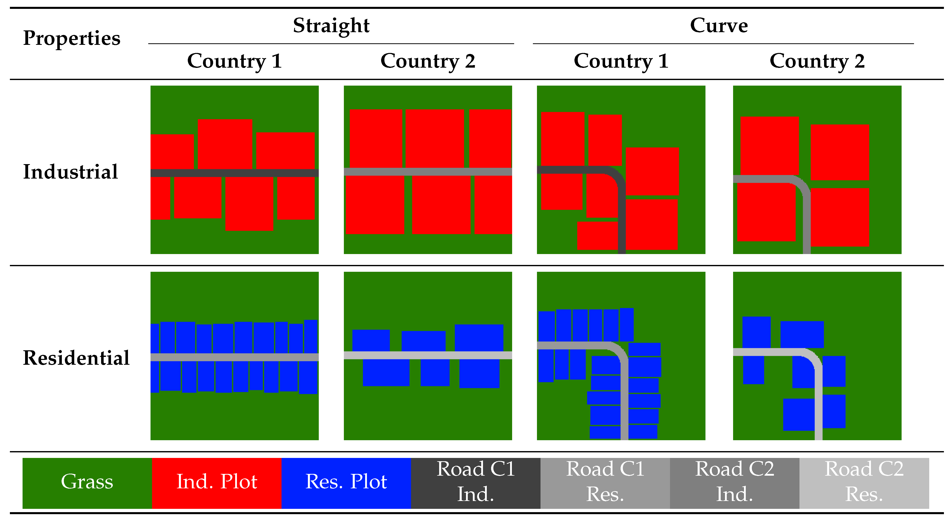
In order to implement a reconstruction function, it is necessary to have access to data that serves as a ground-truth data for the desired appearance of the reconstructed landscape. Based on the assumption of locally flat terrain, the reconstruction is confined to two-dimensional semantics. Based on the environment properties defined in Table A1 a rule-based data generation tool is implemented, creating a total of eight different chunks (straight and curve, two countries, two area types). Samples of this generation technique are shown in Figure 2. The individual segments act as semantic classes and are colored differently for visualization purposes only. Industrial plots are displayed in red, residential plots in blue and grass in green. The roads are grey, with each shade of grey representing a different affiliation to country and area type combination. Images measuring 256 by 256 pixels are used at this point. As indicated in the work’s objective, no real-world data is employed as the baseline so far. Nevertheless, it is still possible to obtain data for this purpose from sources such as OpenStreetMap [41].
In principle, the rule-based generator could be used to rebuild this layer directly. However, such a construction would rely heavily on the creator’s implicit knowledge rather than on rules learned from ground-truth data. Therefore, the following sections present our construction approach, which is based on learned rules developed using the created ground-truth data.
The problem is abstracted into an interpolating and extrapolating task. As mentioned earlier, some explicit information can be extracted from the input to serve as a guideline for reconstructing unknown areas. This is a common image processing task called inpainting. For this task we use the neural network architecture proposed in "MAT: Mask-Aware Transformer for Large Hole Image Inpainting" by [42]. The proposed methodology is based on the generative adversarial network (GAN) architecture and uses a transformer for the inpainting task. The original architectural design is adapted to accommodate varying input and output formats. In its original state, the input and output use RGB images. When it is used to reconstruct class-based landuse data, for example, where each color represents a class, the output may contain invalid classes and other artefacts. This issue is resolved by utilizing additional output formats, such as one-hot encoding. The implementation of one-hot encoding ensures the elimination of ambiguous color values, thereby guaranteeing the production of exclusively valid classes. This, in turn, results in a simplification of both the training process and the subsequent post-processing stage. In order to facilitate the training of the network with one-hot-encoded landuse data, a minor adjustment is made to the loss calculation. The perceptual loss is replaced by cross-entropy loss. Furthermore, the output layer and the corresponding activation function is substituted accordingly. A similar change is implemented at the input stage of the inpainting neural network architecture. Here, the network is prepared to use the original RGB image with a mask to indicate where inpainting is required. The single RGB-Image input is modified to accommodate new data types, including one-hot encoding and black and white images for heightmaps. The number of input and output classes can differ in order to train on classes that will not be generated, such as the road. Finally, the existing convolution implementation is made variable to allow for the use of multiple input maps. In order to judge the training process, the before used Fréchet Inception Distance (FID) is replaced by the mean intersection over union (MiOU) score [43,44].
It was determined that, given the training data is less complex than the data for which the architecture was designed, the discriminator network required a reduction in size by almost half of its original dimensions. Furthermore, it is necessary to adopt the learning rates. Semantic data label smoothing [45] is introduced to improve training.
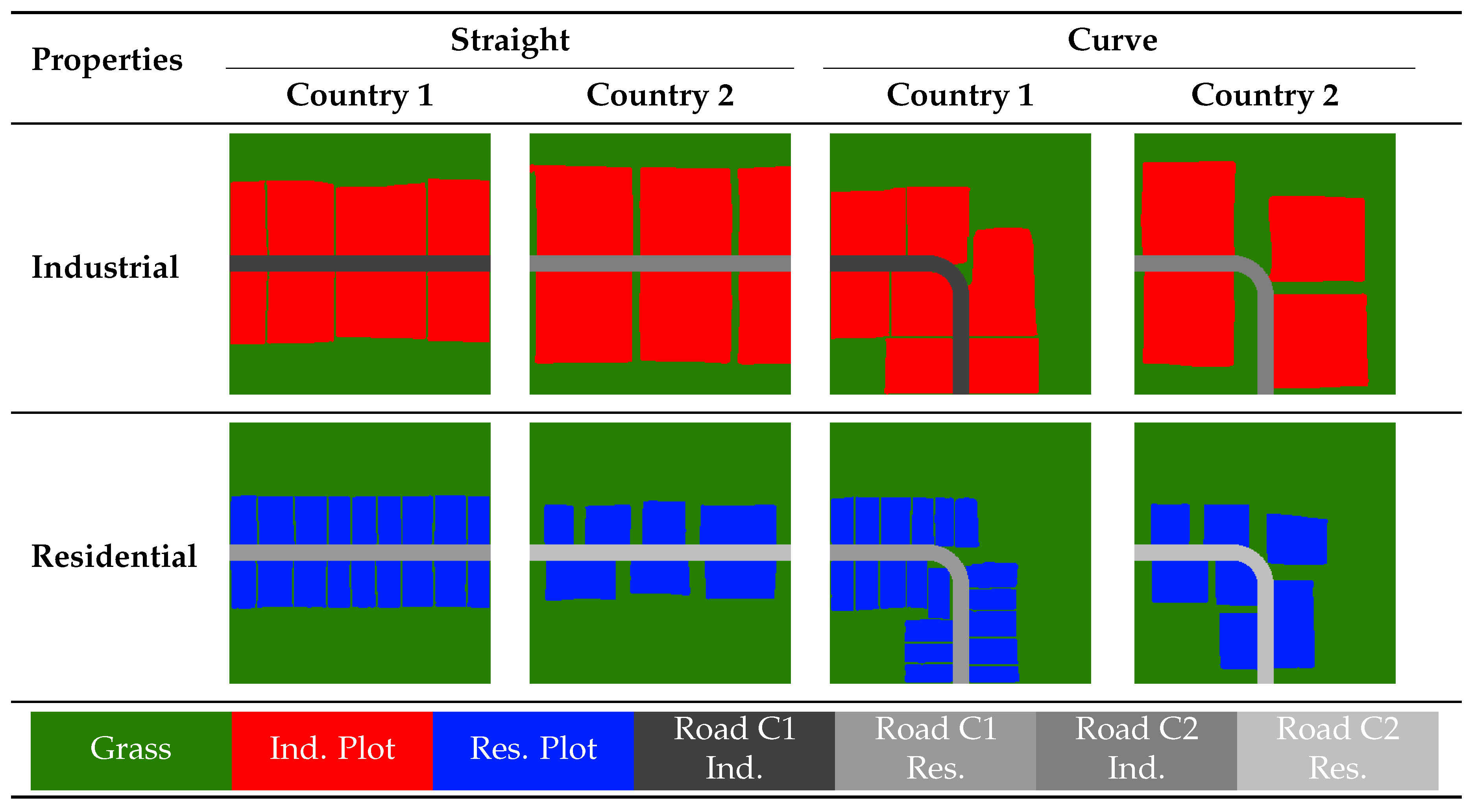
The network was trained for a total of 110 epochs. At this point, there are indications that the training process may be entering a phase of overfitting. The generator is used alone to create landuse samples just with the input of a road course defined by the OpenDRIVE file and the relevant hyperparameters. Any defects that occur, such as holes in individual plots, are repaired with minimal automatic post-processing. Figure 3 displays eight sampled landuse maps. These are used in further reconstruction of the environments, as the ones shown are in the generation of the dataset.
2.3. 3D Semantics Generation - Semantic City
The map-based data constitutes the foundation for the subsequent layer, namely the 3D semantics. In this layer, the position of simple three-dimensional (3D) objects, such as individual trees and props, is defined. In addition, the structure and attributes of more complex elements, including buildings, are specified. We use CityGML [46,47] to represent this information. CityGML is an open standard of the Open Geospatial Consortium (OGC) that has the capacity to represent landscapes through a variety of different modules with varying levels of detail.
This standard is chosen for several reasons. CityGML is a comprehensive model that can describe a wide range of urban and landscape elements, including buildings, transportation infrastructure, vegetation, water bodies, and terrain. Its many thematic modules permit the detailed representation of different aspects of a city or 3D environment, thereby ensuring that all relevant components, such as roofs, facades, road areas, and vegetation types, can be modelled consistently. The schema may be extended with custom Application Domain Extensions (ADEs), rendering it suitable for specialized use cases that require additional attributes or new object types. CityGML is an XML-based open standard that is both machine-readable and widely supported, thereby enabling reliable data exchange between tools, frameworks, and institutions. The aforementioned properties of CityGML render it a robust foundation for the structuring and storage of the semantic 3D information that is required in our framework.
In order to transform the existing data into a CityGML representation, incorporating both input and previously reconstructed information, a range of tools are employed. The tool r:trån [48,49,50] developed at TU Munich is utilized for the purpose of converting OpenDRIVE files to a CityGML representation. The creation of buildings in CityGML is facilitated by the utilization of Random3DCity [51] functions, which have been adapted for this purpose.
Subsequent to the aforementioned conversion, rule-based, procedural modelling approaches are employed for the reconstruction of various components of the scene, in a manner similar to [34] and [35]. In this layer, rule-based approaches are chosen to enhance the controllability of reconstruction. The restriction of possibilities has the advantage of obviating the necessity for implementing sanity checks. Furthermore, the transfer of parametrized objects to a formalized representation, such as CityGML, is thereby rendered more straightforward.
The placement of buildings is governed by a set of rules, the majority of which are defined by environmental properties in Table A1. Nevertheless, it is feasible to derive these regulations from real-world data from sources as indicated in [52,53]. The general parameter ranges are established with minimum and maximum values for the length, width, and number of storeys of the building. Additionally, parameters for the definition of roof type, the placement of windows and doors are set. The placement of buildings on the existing plots is determined by iterating through the existing landuse. For each plot, a rectangle is determined, which fits into the plot boundaries and thereby determine the boundaries of the building. Respecting the boundaries, parameters for the building are randomly sampled from the established ranges. These parameters determine the shape of the building and the placement of additional models, such as windows and doors. Street lights are placed along the road to serve as street furniture. To make the scene more realistic, the positions of the street lights along the road are partly randomized. Trees are placed randomly throughout the scene, respecting the outline of the buildings and the road, based on a specified vegetation density.
2.4. Detailing of the Generated Environment
Following the establishment of the 3D semantics, the final layer - the detailing stage - serves to integrate all components. In this step, the initial ODR input, heightmap, landuse information, and the semantic 3D environment are assembled into a coherent, detailed 3D scene. This layer is structured into two parts. First, preparing the data for import into any 3D simulation environment and second, finalizing it within the chosen simulation platform. These steps work together to transform the abstract semantic representation into a fully realized, simulation-ready 3D environment. This split is introduced to make the simulation platform independent to a certain degree, and to increase modularity, albeit at the cost of additional input and output parsing overhead.
The topology is constructed from the heightmap using a polygonal mesh. The heightmap has a resolution of 256 by 256 pixels, representing an area of 200 by 200 meters. The landuse map is one pixel smaller in size because the heightmap defines the corner positions of each grid cell, while the landuse image defines the cell itself. Road surfaces are not defined by the landuse map, but rather specified in a higher geometric detail through the CityGML r:trån definition. This definition may be directly interpreted as polygonal surfaces. Nevertheless, the landuse road class remains a requisite factor in determining the locations of road transitions. It is evident that, due to the nature of r:trån road geometry being continuous whilst the heightmap is discrete, the presence of gaps would be inevitable in the absence of correction. The resolution of this issue necessitated the development of a stitching algorithm, the function of which is to create surfaces that connect the road borders present in the landuse map to the outermost curves of the r:trån road definition. For each point on these curves, the corresponding grid cell is identified, and polygons are drawn to connect all points that are required. Upon the entry of a new cell, any pending polygon sections are closed.
The generation of buildings is achieved through the direct interpretation of surfaces defined within the CityGML file. The surfaces are triangulated into polygonal meshes. These meshes are then combined with predefined high-resolution 3D objects.
The selection of 3D objects and the later application of materials are governed by a mapping system that links metadata - such as country, area type, and object category - to a distribution. This distribution delineates the probability of spawning specific props or selecting particular materials. The system allows for realistic variation, which would be impossible with a single fixed choice. For example, while two countries might generally use fundamentally different materials for pavements, each country would still use a multitude of different variants with different probabilities. For now, these distributions have to be defined using expert knowledge, but they can also be learnt from real-world data. Therefore, the library is initially created manually.
Two principal methodologies can be employed for the incorporation of three-dimensional objects into the scene. The objects may be embedded directly in the glTF file, or nodes containing the metadata can be created for use in spawning the three-dimensional objects inside the simulation software later. The choice depends on the simulation environment and the intended use of the objects. In instances where the simulation supports direct import and the object does not necessitate additional features or functionality, embedding is a viable option. However, embedding increases file size and consumes more resources during import. In this instance, the second option is employed to distinctly separate the information generation process from the finalization of the environment. All three-dimensional objects are prepared in Unreal Engine as blueprints within a designated library. These blueprints are then inserted during the loading process of the environment. During the process of spawning, the metadata of the dummy nodes is utilized to adapt the 3D objects. In general, metadata attached to the nodes transfers information across tools, such as material selection or segmentation classes. In this final assembly of the environments, high-resolution 3D models are employed for the modelling of the windows [54], the doors [55], the trees [56] and streetlights [57,58]. Furthermore models and materials of Quixel Megascans [59] are used. In order to enhance the realism and aesthetic appeal of the materials, a technique known as texture bombing is employed on select materials.
The final target output format is a three-dimensional environment that is ready to be simulated in the open-source CARLA simulator [21]. In this paper CARLA 0.10.0 is used, which is based on Unreal Engine 5 [20], in order to provide support for recent advancements in rendering techniques, including the Nanite system. The incorporation of such a system has the potential to enhance the framework’s resilience and adaptability to future changes.
Following the transformation of the data into the agnostic 3D format GLTF, its import into CARLA is facilitated by a bespoke import pipeline based on glTFRuntime [60]. The glTFRuntime pipeline is significantly modified to enable the saving of parts of the environment, as well as to interpret additional metadata embedded within the created 3D environments. All elements of the environment are automatically interpreted and prepared for use within CARLA. This preparation involves the establishment of collision properties, the placement of predefined three-dimensional objects as previously referenced, and the allocation of suitable materials. In order to capture synthetic sensor data from the environments, it is necessary to combine multiple chunks in order to create a cohesive street network. This will ensure that route generation is smooth and that roads do not abruptly end. An example of such a street network is illustrated in Figure 4. Each chunk is generated individually, allowing for flexibility and customization in the reconstruction process.
3. Results
Based on the proposed generation framework, four environments are created for each configuration defined earlier. These environments serve as the basis for generating camera data, accompanied by semantically segmented ground-truth data with CARLA. Sample frames showcasing these generated environments are displayed in Figure 5. The whole dataset, named "LGM dataset", is published along with this work in [61]. In total, the dataset contains 2388 images. The distribution of generated images across the generated environments is shown in Table A2.
To validate the approach, two methodologies may be employed. Firstly, the environments can be assessed for realism. This task proves challenging, as purely synthetic environments may lack real-life counterparts, necessitating comparisons of distributions—such as the placement of certain elements. Evaluating the entire environment in this manner presents difficulties due to the multitude of possible distributions that could be analyzed. It is more manageable to perform this assessment on individual reconstruction layers, as demonstrated with the generation of the landuse map.
The second validation method focuses on usability rather than strict realism. While validating for realism assumes that data closest to reality provides the best training and validation outcomes, one could argue that synthetic data may still be useful, despite not closely resembling realistic sensor data from actual test drives. The evaluation of the usefulness of the system is achieved by training a segmentation neural network using various mixtures of realistic and synthetic data. The accuracy of the network is monitored throughout the training process. This kind of validation is done in [12,13,36], and [27]. The objective is to ascertain the extent to which more expensive real-world data may be replaced with cheaper synthetic alternatives while maintaining accuracy in model performance.
Similar to [12,27] the segmentation accuracies are analyzed per class and combined. Additionally we analyzed the training process, varying both the number of images used for training and the ratio of real and synthetic data in the training dataset, while validating only on real data. The network chosen to be trained is Yolo-v8-n [40]. We chose the KITTI-360 dataset [39] as our real dataset. The segmentation classes trained on are road, sidewalk, building, pole, vegetation, terrain, and sky.
The neural network is trained 300 epochs each time. For each configuration 5 different seeds are used. The number of images utilized for training purposes is determined to be 100, 500, and 2000 in total. We varied the ratio of real to synthetic data in steps, later adding some steps to spotlight the region where degradation starts to happen. Real/Synth ratio means, that real data is used for the training process. Every trained network is validated at every epoch on 2000 images sampled randomly from all available drives of the KITTI-360 dataset, which were not used during training.
The global accuracies of the individual trainings are shown in Figure 6. The specific global accuracies together with the segmentation accuracy of each class and the mean per-class accuracy of epoch 300 are displayed in Table 1. As expected, with fewer images per epoch, the training process is slower, as all learning curves are more gradual. In addition, an increase in standard deviation is observed. In general, the greater the amount of synthetic data introduced, the greater the increase in standard deviation and the greater the decrease in accuracy. Figure 7 shows the Pareto front of the final accuracies at epoch 300 for the different Real/Synth ratios. The degradation in accuracy becomes significant at different ratios depending on the dataset size. For a training set of 2000 images, up to of the data can be replaced with only an approximately drop in accuracy. In the 500-image dataset, a similar decrease of about occurs already at replacement. In contrast, the 100-image dataset exhibits a much more pronounced decline: Starting from an initial accuracy of , performance drops by roughly when of the real data is replaced by synthetic data. Overall, the smallest dataset shows higher standard deviations, indicating increased training instability.
When analyzing accuracies on a per-class basis in Table 1, using the mean of all class-wise accuracies with equal weighting across classes, the observed degradation is qualitatively similar but quantitatively stronger. Nevertheless, a substantial portion of the data can still be replaced without a significant loss in performance. Classes such as pole are difficult to segment, exhibiting consistently low accuracy across all training configurations. Other classes achieve considerably better results. In the 2000-image and 500-image datasets, certain classes — road and building — are even segmented slightly more accurately when training is performed with partially synthetic data.
4. Conclusion
This work presents a modular, flexible, and easily scalable framework to generate synthetic 3D environments. The fast and cheaply generated 3D environments are used to produce high-quality synthetic sensor data, in conjunction with consistent ground truth. The findings from the validation experiments demonstrate that the synthetic data generated has the capacity to substitute a significant proportion of real data prior to the occurrence of perceptible accuracy degradation. This finding suggests that the generated environments are capable of capturing the relevant structural and semantic properties needed for training and validating perception models. Synthetic data and our underlying framework present a promising alternative to the usage of purely real-world data collection, as real-world data is connected to high costs, exhaustive manual work, and - in some cases - even unethical and dangerous techniques. Nevertheless, the results of the study indicate further possibilities for improvement.
We show the usage of inpainting networks for maps used to reconstruct 3D environments. Our presented technique works, but may be utilized further. Additional map-based data, such as the heightmap, may be generated. This data may serve as the foundation for the generation of water maps or further data, which can be abstracted to a 2D map. As the data to be generated can be diverse, the architecture may need additional changes. Additionally, automated hyperparameter tuning should be explored.
CityGML proves to be a powerful foundation for representing the whole static 3D environment semantically. For now, a variety of different objects are introduced, which may be expanded in the future to fill the scene with life.
This holds true for the detailing stage. Here, additional components should be introduced, such as foliage and depth to certain materials, with, for example, virtualized geometry through systems like Unreal Engine’s Nanite system. This would introduce more (wanted) noise to the generated 3D environments, making them more variable. This addition is also interesting for generating LiDAR data from the given 3D environments.
Our validation shows that in our experiments, approximately up to 90% of the real data can be replaced by our synthetic data without significant accuracy degradation, depending on the training configuration. Our extensive training results with different Real/Synth ratios and training set sizes give a good indication that our data can be used in varying situations. A key contribution is the LGM dataset we present along this work in [61]. The dataset offers a total of 2388 color images along with a semantic segmentation in 7 classes.
For future research, we identified three main goals we want to explore further. Firstly, domain shifts or general variations of the generated environments are of great interest. In this regard, the framework may be further extended by introducing additional features and components in the individual modules. In the detailing layer, dynamic effects such as weather and day/night cycles may be introduced. In the case of the map-based data reconstruction and 3D semantics, further areas may be included in the generation as well as further use cases. Two interesting use cases are agricultural and maritime applications, where map-based data, such as currents or, in the case of agriculture, soil conditions can be reconstructed along with relevant scenery.
Secondly, we would like to explore further techniques for the generation of the different layers. In the case of placement of scene components or map-based generation approaches, such as stated in [62], can be implemented. This would enhance the possibilities and the flexibility of the proposed framework, as more diverse input data may be introduced. Also, environments could be represented with varying granularity, which may be more suitable for a specific use case. We plan on incorporating dynamic objects with interactions, as shown in [63] in the framework as well.
Thirdly, although the data produced is already usable in its current state, we would like to introduce real data as the baseline on which we train or define every single generation step. For this, the groundwork is already laid, as the layers are designed to encompass real data sources, as indicated. All of these points would greatly enhance the possibilities of the framework for generating scenarios, which can cover a great portion of the ODD of an ADAS functionality. As previously mentioned, this could lead to further advancements in the fields of ADAS fuzzing and ODD exploration. Consequently, this could facilitate targeted searches specifically targeting edge cases. Such a possibility would increase the safety for autonomous vehicles.
Author Contributions
Conceptualization, T.T., J.D., M.E. and J.A.; methodology, T.T., J.D., L.L., B.K. and T.B.; software, T.T., J.D. and L.L.; validation, T.T. and J.D.; formal analysis, T.T. and J.D.; investigation, T.T.; resources, T.T., J.D. and B.K.; data curation, T.T. and J.D.; writing—original draft preparation, T.T.; writing—review and editing, T.T., J.D., L.L., B.K., T.B., M.E. and J.A.; visualization, T.T. and J.D.; supervision, M.E. and J.A.; project administration, T.T., M.E. and J.A.; funding acquisition, M.E. and J.A. All authors have read and agreed to the published version of the manuscript.
Funding
This research received no external funding.
Data Availability Statement
The original data presented in the study are openly available in LGM_SemanticSegmentationDataset_1 at https://doi.org/10.5281/ZENODO.17949756.
Acknowledgments
Simulations were performed with computing resources granted by RWTH Aachen University under project rwth1892.
Conflicts of Interest
The authors declare no conflicts of interest.
Appendix A

Table A1.
Overview of environment properties
| Properties | Country 1 | Country 2 | ||
|---|---|---|---|---|
| Industrial | Residential | Industrial | Residential | |
| General ground type | Green grass | Green grass | Green grass | Green grass |
| Road markings | White | White | Yellow | Yellow |
| Plot size | Medium | Long, narrow | Large | Medium |
| House size | Large warehouses | Tall inner-city style | Large warehouses | Small rural |
| House material | Sheet metal | Red brick | Sheet metal | Flagstone |
| Windows | Few | Many | Few | Normal |
| Ground type | Rubble | Fit green grass | Rubble | Fit green grass |
| Street light type | Virginia street light | Virginia street light | New York street light | New York street light |
| Tree density | Low | High | Low | High |
Table A2.
Distribution of the generated images in the accompanying dataset across the four 3D environments created.
Table A2.
Distribution of the generated images in the accompanying dataset across the four 3D environments created.
| Country 1 Industrial | Country 1 Residential | Country 2 Industrial | Country 2 Residential |
|---|---|---|---|
| 575 | 626 | 557 | 630 |
Abbreviations
The following abbreviations are used in this manuscript:
| AD | Automated Driving |
| ADAS | Advanced Driver Assistance Systems |
| AV | Automated Vehicle |
| GAN | Generative Adversarial Networks |
| IND | Industrial |
| ODD | Operational Design Domain |
| ODR | OpenDRIVE |
| OSC | OpenSCENARIO |
| MBSE | Model-Based Systems Engineering |
| RES | Residential |
| SBSE | Scenario-Based Systems Engineering |
| STD | Standard Deviation |
References
- Lou, G.; Deng, Y.; Zheng, X.; Zhang, M.; Zhang, T. Testing of Autonomous Driving Systems: Where Are We and Where Should We Go? In Proceedings of the Proceedings of the 30th ACM Joint European Software Engineering Conference and Symposium on the Foundations of Software Engineering, Singapore Singapore, 2022; pp. 31–43. [Google Scholar] [CrossRef]
- Song, Q.; Bensoussan, A.; Mousavi, M.R. Synthetic versus Real: An Analysis of Critical Scenarios for Autonomous Vehicle Testing. Automated Software Engineering 2025, 32, 37. [Google Scholar] [CrossRef]
- Wäschle, M.; Thaler, F.; Berres, A.; Pölzlbauer, F.; Albers, A. A Review on AI Safety in Highly Automated Driving. Frontiers in Artificial Intelligence 2022, 5, 952773. [Google Scholar] [CrossRef] [PubMed]
- Mehlhorn, M.A.; Richter, A.; Shardt, Y.A. Ruling the Operational Boundaries: A Survey on Operational Design Domains of Autonomous Driving Systems. IFAC-PapersOnLine 2023, 56, 2202–2213. [Google Scholar] [CrossRef]
- ASAM, e. V. ASAM OpenSCENARIO®. 2022. Available online: https://www.asam.net/standards/detail/openscenario/v200/.
- ASAM, e. V. ASAM OpenDRIVE®. 2024. Available online: https://www.asam.net/standards/detail/opendrive/.
- ASAM, e. V. ASAM OpenMATERIAL® 3D. 2025. Available online: https://www.asam.net/standards/detail/openmaterial/.
- Temmen, T.; Meyer, M.A.; Wachtmeister, L.; Zabihi, M.; Kugler, C.; Christiaens, S.; Rumpe, B.; Andert, J. Application of Model-Based Systems Engineering Methods in Virtual Homologation Procedures for Automated Driving Functions. In Automatisiertes Fahren 2024; Heintzel, A., Ed.; Springer Fachmedien Wiesbaden: Wiesbaden, 2024; pp. 1–10. [Google Scholar] [CrossRef]
- Meyer, M.A.; Silberg, S.; Granrath, C.; Kugler, C.; Wachtmeister, L.; Rumpe, B.; Christiaens, S.; Andert, J. Scenario- and Model-Based Systems Engineering Procedure for the SOTIF-Compliant Design of Automated Driving Functions. In Proceedings of the 2022 IEEE Intelligent Vehicles Symposium (IV), Aachen, Germany, 2022; pp. 1599–1604. [Google Scholar] [CrossRef]
- Wang, Y.; Xing, S.; Can, C.; Li, R.; Hua, H.; Tian, K.; Mo, Z.; Gao, X.; Wu, K.; Zhou, S.; et al. Generative AI for Autonomous Driving. Frontiers and Opportunities 2025, arXiv:cs. [Google Scholar] [CrossRef]
- Greff, K.; Belletti, F.; Beyer, L.; Doersch, C.; Du, Y.; Duckworth, D.; Fleet, D.J.; Gnanapragasam, D.; Golemo, F.; Herrmann, C.; et al. Kubric: A Scalable Dataset Generator. In Proceedings of the 2022 IEEE/CVF Conference on Computer Vision and Pattern Recognition (CVPR), New Orleans, LA, USA, 2022; pp. 3739–3751. [Google Scholar] [CrossRef]
- Richter, S.R.; Vineet, V.; Roth, S.; Koltun, V. Playing for Data: Ground Truth from Computer Games. In Computer Vision – ECCV 2016; Leibe, B., Matas, J., Sebe, N., Welling, M., Eds.; Springer International Publishing: Cham, 2016; Vol. 9906, pp. 102–118. [Google Scholar] [CrossRef]
- Nowruzi, F.E.; Kapoor, P.; Kolhatkar, D.; Hassanat, F.A.; Laganiere, R.; Rebut, J. How Much Real Data Do We Actually Need: Analyzing Object Detection Performance Using Synthetic and Real Data. arXiv 2019, arXiv:1907.07061. [Google Scholar] [CrossRef]
- Wen, B.; Xie, H.; Chen, Z.; Hong, F.; Liu, Z. 3D Scene Generation: A Survey. arXiv 2025, arXiv:2505.05474. [Google Scholar] [CrossRef]
- Bai, X.; Luo, Y.; Jiang, L.; Gupta, A.; Kaveti, P.; Singh, H.; Ostadabbas, S. Bridging the Domain Gap between Synthetic and Real-World Data for Autonomous Driving. arXiv 2023, arXiv:cs. [Google Scholar] [CrossRef]
- Sun, P.; Kretzschmar, H.; Dotiwalla, X.; Chouard, A.; Patnaik, V.; Tsui, P.; Guo, J.; Zhou, Y.; Chai, Y.; Caine, B.; et al. Scalability in Perception for Autonomous Driving: Waymo Open Dataset. In Proceedings of the 2020 IEEE/CVF Conference on Computer Vision and Pattern Recognition (CVPR), Seattle, WA, USA, 2020; pp. 2443–2451. [Google Scholar] [CrossRef]
- Koopman, P.; Widen, W. Safety Ethics for Design and Test of Automated Driving Features. IEEE Design & Test 2024, 41, 17–24. [Google Scholar] [CrossRef]
- Hu, A.; Russell, L.; Yeo, H.; Murez, Z.; Fedoseev, G.; Kendall, A.; Shotton, J.; Corrado, G. GAIA-1: A Generative World Model for Autonomous Driving. Comment: Technical Report 2023, arXiv:cs. [Google Scholar] [CrossRef]
- Projekt, P. PEGASUS METHOD An Overview. 2019. Available online: https://www.pegasusprojekt.de/files/tmpl/Pegasus-Abschlussveranstaltung/PEGASUS-Gesamtmethode.pdf.
- Epic Games, I. Unreal Engine. 2025. Available online: https://www.unrealengine.com/en-US.
- Dosovitskiy, A.; Ros, G.; Codevilla, F.; Lopez, A.; Koltun, V. CARLA: An Open Urban Driving Simulator. In Proceedings of the Proceedings of the 1st Annual Conference on Robot Learning Proceedings of Machine Learning Research PMLR; Levine, S., Vanhoucke, V., Goldberg, K., Eds.; 2017; Vol. 78, pp. 1–16. [Google Scholar]
- Yang, Z.; Chai, Y.; Anguelov, D.; Zhou, Y.; Sun, P.; Erhan, D.; Rafferty, S.; Kretzschmar, H. SurfelGAN: Synthesizing Realistic Sensor Data for Autonomous Driving. In Proceedings of the 2020 IEEE/CVF Conference on Computer Vision and Pattern Recognition (CVPR), Seattle, WA, USA, 2020; pp. 11115–11124. [Google Scholar] [CrossRef]
- Gaidon, A.; Wang, Q.; Cabon, Y.; Vig, E. VirtualWorlds as Proxy for Multi-object Tracking Analysis. In Proceedings of the 2016 IEEE Conference on Computer Vision and Pattern Recognition (CVPR), Las Vegas, NV, USA, 2016; pp. 4340–4349. [Google Scholar] [CrossRef]
- Cabon, Y.; Murray, N.; Humenberger, M. Virtual KITTI 2. arXiv 2020, arXiv:2001.10773. [Google Scholar] [CrossRef]
- Xie, Z.; Zhang, J.; Li, W.; Zhang, F.; Zhang, L. S-NERF: NEURAL RADIANCE FIELDS FOR STREET. 2023. [Google Scholar]
- Richter, S.R.; Hayder, Z.; Koltun, V. Playing for Benchmarks. In Proceedings of the 2017 IEEE International Conference on Computer Vision (ICCV), Venice, 2017; pp. 2232–2241. [Google Scholar] [CrossRef]
- Ros, G.; Sellart, L.; Materzynska, J.; Vazquez, D.; Lopez, A.M. The SYNTHIA Dataset: A Large Collection of Synthetic Images for Semantic Segmentation of Urban Scenes. In Proceedings of the 2016 IEEE Conference on Computer Vision and Pattern Recognition (CVPR), Las Vegas, NV, USA, 2016; pp. 3234–3243. [Google Scholar] [CrossRef]
- Li, Y.; Jiang, L.; Xu, L.; Xiangli, Y.; Wang, Z.; Lin, D.; Dai, B. MatrixCity: A Large-scale City Dataset for City-scale Neural Rendering and Beyond. In Proceedings of the 2023 IEEE/CVF International Conference on Computer Vision (ICCV), Paris, France, 2023; pp. 3182–3192. [Google Scholar] [CrossRef]
- Kim, S.; Liu, M.; Rhee, J.J.; Jeon, Y.; Kwon, Y.; Kim, C.H. DriveFuzz: Discovering Autonomous Driving Bugs through Driving Quality-Guided Fuzzing. In Proceedings of the Proceedings of the 2022 ACM SIGSAC Conference on Computer and Communications Security, Los Angeles CA USA, 2022; pp. 1753–1767. [Google Scholar] [CrossRef]
- Li, G.; Li, Y.; Jha, S.; Tsai, T.; Sullivan, M.; Hari, S.K.S.; Kalbarczyk, Z.; Iyer, R. AV-FUZZER: Finding Safety Violations in Autonomous Driving Systems. In Proceedings of the 2020 IEEE 31st International Symposium on Software Reliability Engineering (ISSRE), Coimbra, Portugal, 2020; pp. 25–36. [Google Scholar] [CrossRef]
- Yang, H.; Zhou, Y.; Chen, T. SimADFuzz: Simulation-feedback Fuzz Testing for Autonomous Driving Systems. In ACM Trans. Softw. Eng. Methodol.; 2025. [Google Scholar] [CrossRef]
- Lin, S.; Chen, F.; Xi, L.; Wang, G.; Xi, R.; Sun, Y.; Zhu, H. TM-fuzzer: Fuzzing Autonomous Driving Systems through Traffic Management. Automated Software Engineering 2024, 31, 61. [Google Scholar] [CrossRef]
- Krautwig, B.; Wans, D.; Li, L.; Temmen, T.; Koch, L.; Eisenbarth, M.; Andert, J. Navigating the Trade-Offs: A Quantitative Analysis of Reinforcement Learning Reward Functions for Autonomous Maritime Collision Avoidance. Journal of Marine Science and Engineering 2025, 13, 2233. [Google Scholar] [CrossRef]
- Zhou, M.; Wang, Y.; Hou, J.; Zhang, S.; Li, Y.; Luo, C.; Peng, J.; Zhang, Z. SceneX: Procedural Controllable Large-Scale Scene Generation. In Proceedings of the Proceedings of the Thirty-Ninth AAAI Conference on Artificial Intelligence and Thirty-Seventh Conference on Innovative Applications of Artificial Intelligence and Fifteenth Symposium on Educational Advances in Artificial Intelligence; AAAI Press; AAAI’25/IAAI’25/EAAI’25, 2025. [Google Scholar] [CrossRef]
- Raistrick, A.; Lipson, L.; Ma, Z.; Mei, L.; Wang, M.; Zuo, Y.; Kayan, K.; Wen, H.; Han, B.; Wang, Y.; et al. Infinite Photorealistic Worlds Using Procedural Generation. In Proceedings of the 2023 IEEE/CVF Conference on Computer Vision and Pattern Recognition (CVPR), Vancouver, BC, Canada, 2023; pp. 12630–12641. [Google Scholar] [CrossRef]
- Tsirikoglou, A.; Kronander, J.; Wrenninge, M.; Unger, J. Procedural Modeling and Physically Based Rendering for Synthetic Data Generation in Automotive Applications. 2017. [Google Scholar] [CrossRef]
- Wrenninge, M.; Unger, J. Synscapes: A Photorealistic Synthetic Dataset for Street Scene Parsing. arXiv 2018, arXiv:1810.08705. [Google Scholar] [CrossRef]
- Sun, T.; Segu, M.; Postels, J.; Wang, Y.; Van Gool, L.; Schiele, B.; Tombari, F.; Yu, F. SHIFT: A Synthetic Driving Dataset for Continuous Multi-Task Domain Adaptation. In Proceedings of the 2022 IEEE/CVF Conference on Computer Vision and Pattern Recognition (CVPR), New Orleans, LA, USA, 2022; pp. 21339–21350. [Google Scholar] [CrossRef]
- Liao, Y.; Xie, J.; Geiger, A. KITTI-360: A Novel Dataset and Benchmarks for Urban Scene Understanding in 2D and 3D. IEEE Transactions on Pattern Analysis and Machine Intelligence 2023, 45, 3292–3310. [Google Scholar] [CrossRef]
- Jocher, G.; Chaurasia, A.; Qiu, J. Ultralytics Yolov8, 2023. Accessed. 2025.
- OpenStreetMap contributors. Planet Dump Retrieved from. 2017. Available online: https://planet.osm.org.
- Li, W.; Lin, Z.; Zhou, K.; Qi, L.; Wang, Y.; Jia, J. MAT: Mask-Aware Transformer for Large Hole Image Inpainting. In Proceedings of the 2022 IEEE/CVF Conference on Computer Vision and Pattern Recognition (CVPR), New Orleans, LA, USA, 2022; pp. 10748–10758. [Google Scholar] [CrossRef]
- Bynagari, N.B. GANs Trained by a Two Time-Scale Update Rule Converge to a Local Nash Equilibrium. Asian Journal of Applied Science and Engineering 2019, 8, 25–34. [Google Scholar] [CrossRef]
- Everingham, M.; Van Gool, L.; Williams, C.K.I.; Winn, J.; Zisserman, A. The Pascal Visual Object Classes (VOC) Challenge. International Journal of Computer Vision 2010, 88, 303–338. [Google Scholar] [CrossRef]
- Szegedy, C.; Vanhoucke, V.; Ioffe, S.; Shlens, J.; Wojna, Z. Rethinking the Inception Architecture for Computer Vision. In Proceedings of the 2016 IEEE Conference on Computer Vision and Pattern Recognition (CVPR), Las Vegas, NV, USA, 2016; pp. 2818–2826. [Google Scholar] [CrossRef]
- O.G.C., V. CityGML. 2025. Available online: https://www.ogc.org/standards/citygml/.
- O.G.C.C., V.; Kolbe, T.H.; Kutzner, T.; Smyth, C.S.; Nagel, C.; Roensdorf, C.; Heazel, C. OGC City Geography Markup Language (CityGML) Part 1: Conceptual Model Standard. 2021. Available online: https://docs.ogc.org/is/20-010/20-010.html.
- Schwab, B.; Beil, C.; Kolbe, T. H. R:Trån. Zenodo. Accessed. 2023. [CrossRef]
- Schwab, B.; Beil, C.; Kolbe, T.H. Spatio-Semantic Road Space Modeling for Vehicle–Pedestrian Simulation to Test Automated Driving Systems. Sustainability 2020, 12, 3799. [Google Scholar] [CrossRef]
- Schwab, B.; Kolbe, T.H. VALIDATION OF PARAMETRIC OPENDRIVE ROAD SPACE MODELS. ISPRS Annals of the Photogrammetry, Remote Sensing and Spatial Information Sciences 2022, X-4/W2-2022, 257–264. [Google Scholar] [CrossRef]
- Biljecki, F.; Ledoux, H.; Stoter, J. GENERATION OF MULTI-LOD 3D CITY MODELS IN CITYGML WITH THE PROCEDURAL MODELLING ENGINE RANDOM3DCITY. ISPRS Annals of the Photogrammetry, Remote Sensing and Spatial Information Sciences 2016, IV-4/W1, 51–59. [Google Scholar] [CrossRef]
- Wysocki, O.; Schwab, B.; Beil, C.; Holst, C.; Kolbe, T.H. Reviewing Open Data Semantic 3D City Models to Develop Novel 3D Reconstruction Methods. The International Archives of the Photogrammetry, Remote Sensing and Spatial Information Sciences 2024, XLVIII-4-2024, 493–500. [Google Scholar] [CrossRef]
- Wysocki, O.; Schwab, B.; Willenborg, B. OloOcki/Awesome-Citygml: Release. Zenodo. Accessed. 2022. [CrossRef]
- OMA. Window. 2025. Available online: https://www.fab.com/listings/78769db1-cc1c-4edb-a1a7-e1b026758aa9.
- DHaupt. Room Door Animation. 2013. Available online: https://sketchfab.com/3d-models/room-door-animation-e85909e80635445b92fb80772af80c84.
- EFX. HIGH QUALITY TREE 6/6. 2023. Available online: https://sketchfab.com/3d-models/high-quality-tree-66-221b8943cc514162a05be24b7ba35430.
- Fan, A. NYC Streetlight 1. 2025. Available online: https://sketchfab.com/3d-models/nyc-streetlight-1-456df4ed4b3241938695eef72b941123.
- Fan, A. Virginia Streetlight 1. 2025. Available online: https://sketchfab.com/3d-models/virginia-streetlight-1-d2ae505054a142a596b1386d0b5f1f98.
- Megascans, Q. Quixel Megascans. 2024. Available online: https://www.fab.com/sellers/Quixel%20Megascans.
- De Ioris, R. glTFRuntime: Unreal Engine Plugin for Loading glTF Files at Runtime. Accessed. 2025.
- Temmen, T.; Debougnoux, J.; Li, L.; Krautwig, B.; Brinkmann, T.; Eisenbarth, M.; Andert, J. TTemmen/LGM_SemanticSegmentationDataset_1: V1.1. Zenodo. Accessed. 2025. [CrossRef]
- He, L.; Aliaga, D. GlobalMapper: Arbitrary-Shaped Urban Layout Generation. In Proceedings of the 2023 IEEE/CVF International Conference on Computer Vision (ICCV), Paris, France, 2023; pp. 454–464. [Google Scholar] [CrossRef]
- Li, L.; Brinkmann, T.; Temmen, T.; Eisenbarth, M.; Andert, J. Multi-Agent Scenario Generation in Roundabouts with a Transformer-enhanced Conditional Variational Autoencoder. arXiv 2025, arXiv:cs. [Google Scholar] [CrossRef]
Figure 1.
Concept of the proposed modular framework for the generation of static 3D environments
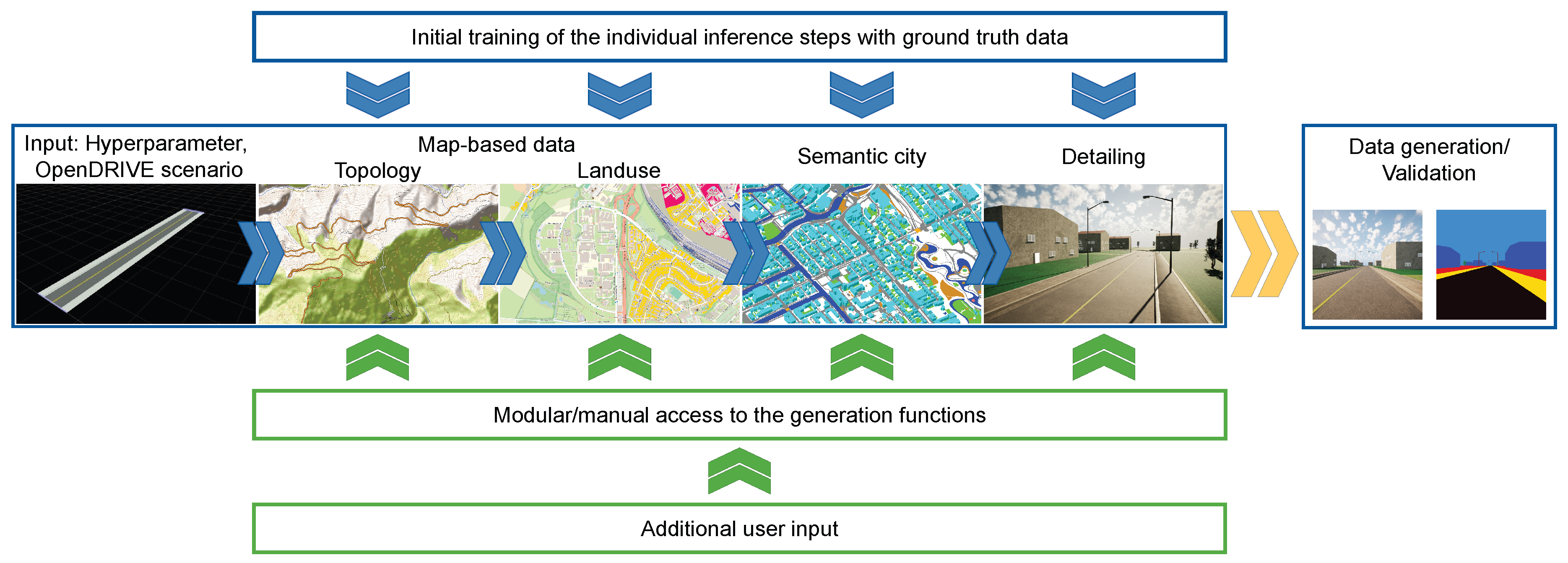
Figure 2.
Samples of the training data for the landuse reconstruction
| Properties | Straight | Curve | |||
| Country 1 | Country 2 | Country 1 | Country 2 | ||
| Industrial | |||||
| Residential | |||||
| GrassInd. PlotRes. PlotRoad C1 Ind.Road C1 Res.Road C2 Ind.Road C2 Res. | |||||
| Grass | Ind. Plot | Res. Plot | Road C1 Ind. | Road C1 Res. | Road C2 Ind. | Road C2 Res. |
Figure 3.
Samples of the training data for the landuse reconstruction
| Properties | Straight | Curve | |||
| Country 1 | Country 2 | Country 1 | Country 2 | ||
| Industrial | |||||
| Residential | |||||
| GrassInd. PlotRes. PlotRoad C1 Ind.Road C1 Res.Road C2 Ind.Road C2 Res. | |||||
| Grass | Ind. Plot | Res. Plot | Road C1 Ind. | Road C1 Res. | Road C2 Ind. | Road C2 Res. |
Figure 4.
Two street networks generated with the framework are shown. (a) Presents an environment generated for country 1 residential. (b) Presents an environment generated for country 2 residential.
Figure 4.
Two street networks generated with the framework are shown. (a) Presents an environment generated for country 1 residential. (b) Presents an environment generated for country 2 residential.
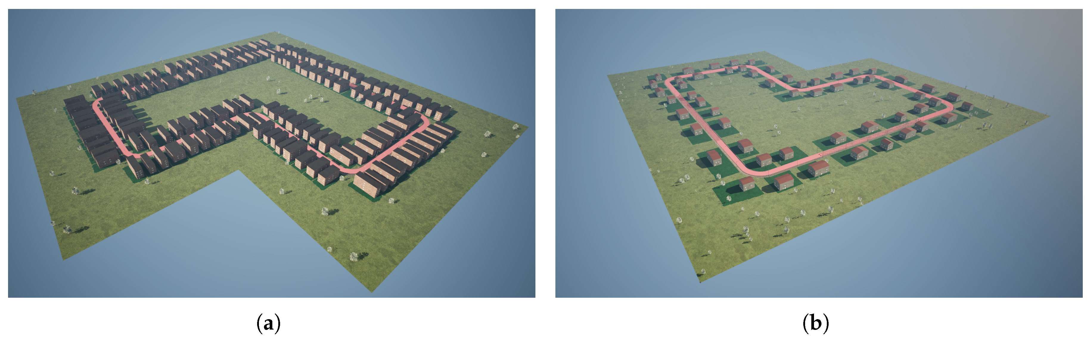
Figure 5.
Four samples of color camera data (top row) and respective semantic segmentation (bottom row) sampled from the four generated environments: Country 1 industrial (a, e), Country 1 residential (b, f), Country 2 industrial (c, g), Country 2 residential (d, h).
Figure 5.
Four samples of color camera data (top row) and respective semantic segmentation (bottom row) sampled from the four generated environments: Country 1 industrial (a, e), Country 1 residential (b, f), Country 2 industrial (c, g), Country 2 residential (d, h).
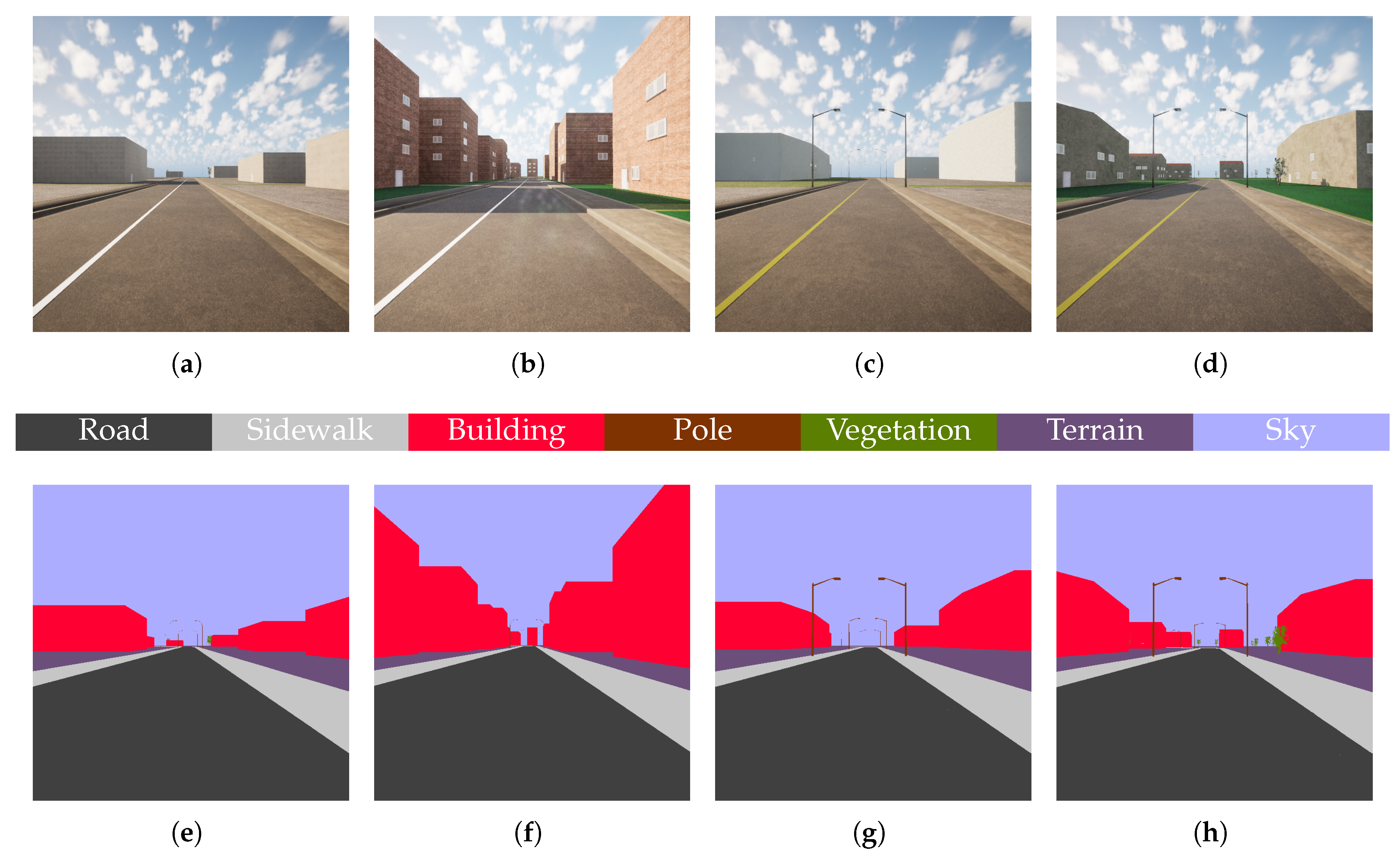
| Road | Sidewalk | Building | Pole | Vegetation | Terrain | Sky |
Figure 6.
Global accuracies along the training process. In the upper row the mean value across the five different seeds is displayed, in the lower row the standard deviation is displayed. Each column corresponds to 100, 500 and 2000 training samples per epoch.
Figure 6.
Global accuracies along the training process. In the upper row the mean value across the five different seeds is displayed, in the lower row the standard deviation is displayed. Each column corresponds to 100, 500 and 2000 training samples per epoch.
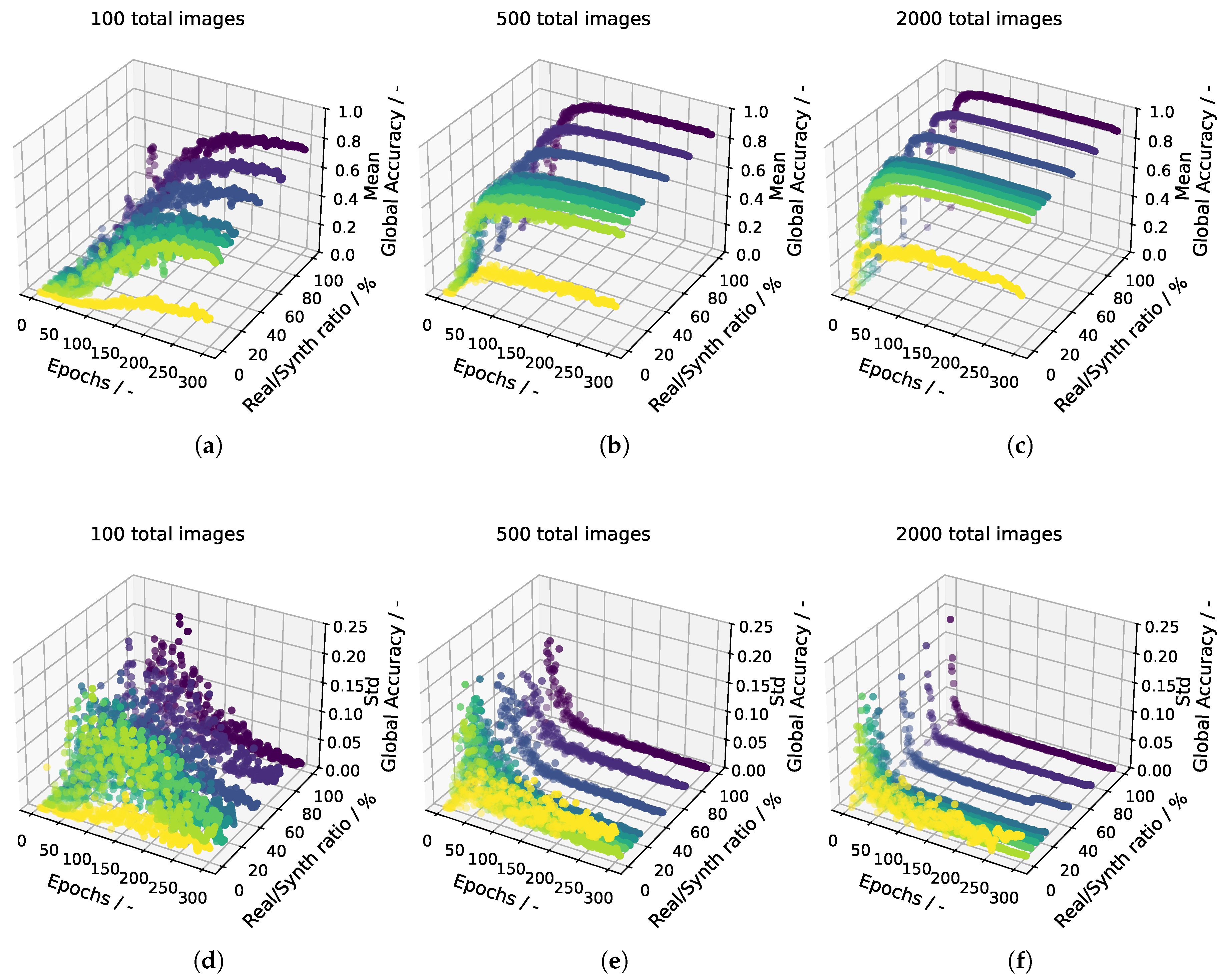
Figure 7.
Mean accuracies with standard deviations at epoch 300 at varying Real/Synth ratios. Each line represents one of the three training dataset sizes used.
Figure 7.
Mean accuracies with standard deviations at epoch 300 at varying Real/Synth ratios. Each line represents one of the three training dataset sizes used.
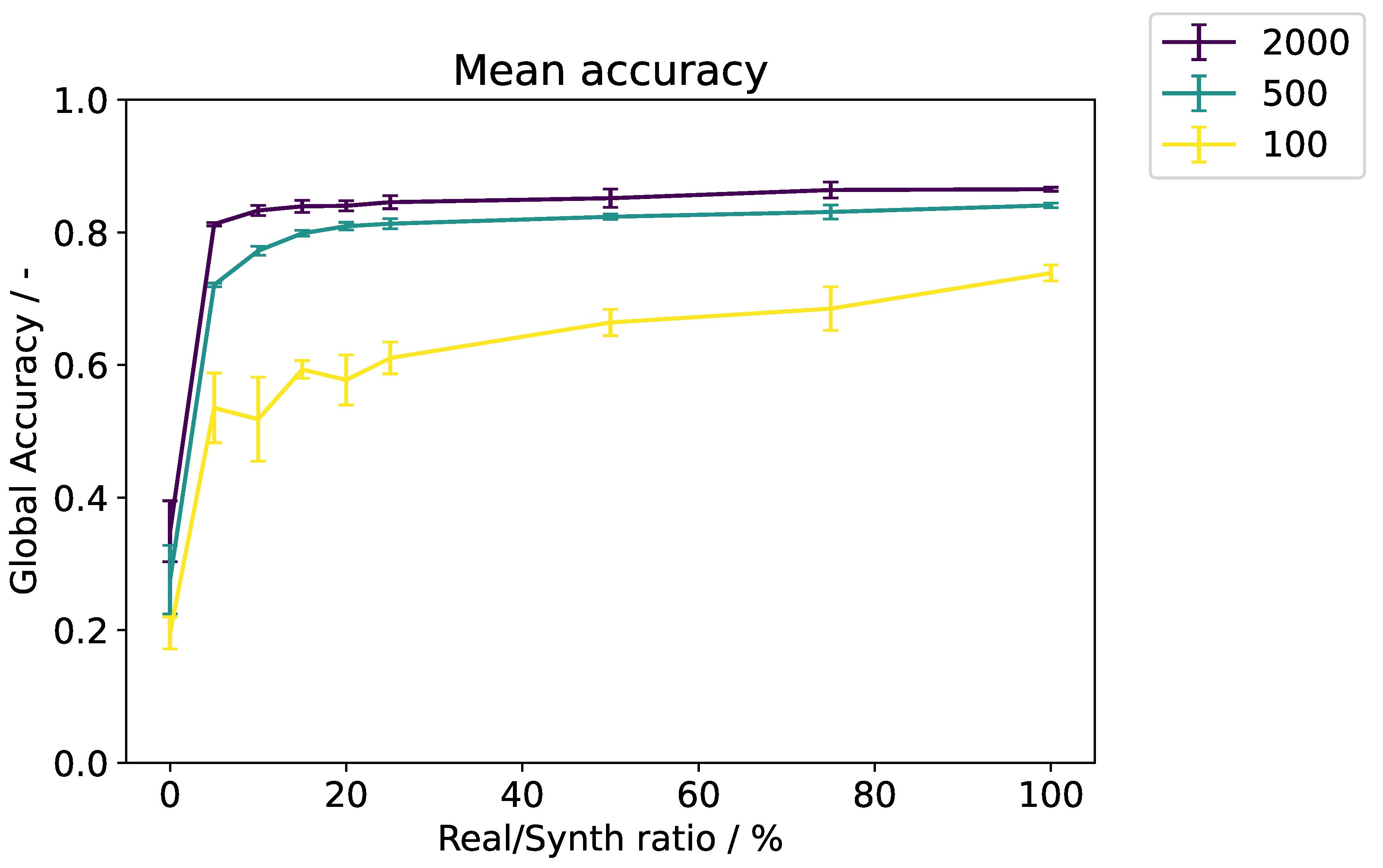
Table 1.
The mean accuracies and their respective standard deviations at epoch 300, with the size of the training set varying. All numerical values are expressed as percentages.
Table 1.
The mean accuracies and their respective standard deviations at epoch 300, with the size of the training set varying. All numerical values are expressed as percentages.
| 2000 training samples | |||||||||
| Real/Synth ratio | Road | Sidewalk | Building | Pole | Vegetation | Terrain | Sky | Per-class accuracy | Global accuracy |
| 100 | |||||||||
| 75 | |||||||||
| 50 | |||||||||
| 25 | |||||||||
| 20 | |||||||||
| 15 | |||||||||
| 10 | |||||||||
| 5 | |||||||||
| 0 | |||||||||
| 500 training samples | |||||||||
| Real/Synth ratio | Road | Sidewalk | Building | Pole | Vegetation | Terrain | Sky | Per-class accuracy | Global accuracy |
| 100 | |||||||||
| 75 | |||||||||
| 50 | |||||||||
| 25 | |||||||||
| 20 | |||||||||
| 15 | |||||||||
| 10 | |||||||||
| 5 | |||||||||
| 0 | |||||||||
| 100 training samples | |||||||||
| Real/Synth Ratio | Road | Sidewalk | Building | Pole | Vegetation | Terrain | Sky | Per-class accuracy | Global accuracy |
| 100 | |||||||||
| 75 | |||||||||
| 50 | |||||||||
| 25 | |||||||||
| 20 | |||||||||
| 15 | |||||||||
| 10 | |||||||||
| 5 | |||||||||
| 0 | |||||||||
Disclaimer/Publisher’s Note: The statements, opinions and data contained in all publications are solely those of the individual author(s) and contributor(s) and not of MDPI and/or the editor(s). MDPI and/or the editor(s) disclaim responsibility for any injury to people or property resulting from any ideas, methods, instructions or products referred to in the content. |
© 2026 by the authors. Licensee MDPI, Basel, Switzerland. This article is an open access article distributed under the terms and conditions of the Creative Commons Attribution (CC BY) license (http://creativecommons.org/licenses/by/4.0/).
Copyright: This open access article is published under a Creative Commons CC BY 4.0 license, which permit the free download, distribution, and reuse, provided that the author and preprint are cited in any reuse.


