
Submitted:
31 December 2025
Posted:
01 January 2026
You are already at the latest version
Abstract
This study investigates and formulates a structured framework to guide deci-sion-making in the remanufacturing of spent electric vehicle (EV) traction motors. With a projected increase in the number of motors reaching end-of-life, the study tack-les key challenges by introducing a data-driven, integrated remanufacturing approach. A predictive algorithm was developed to estimate Remaining Useful Life (RUL) from operational parameters, supported by exploratory data analysis (EDA) that highlight-ed strong inverse relationships between lifespan and stress-related variables such as mechanical load, vibration, and thermal exposure. Various machine learning models including random forest, gradient boosting, and support vector regression yielded moderate predictive performance (mean absolute error ≈ 9.0 km; R² ≈ 0.58), with long short-term memory (LSTM) networks outperforming others (error ≈ 9.1k km; R² ≈ 0.61). These results demonstrate the viability of using predictive analytics to inform reman-ufacturing decisions, contributing to circular economy principles through sustainable EV motor reuse.
Keywords:
MAE—mean absolute error
; MSE—mean square error
; RMSE—root mean square error
; DAQ—data acquisition
; LSTM—long short-term memory
; RNN—recurrent neural network
1. Introduction
Nations momentum toward electrification of transport, driven by emission-reduction targets and bans on new internal combustion engine vehicles by 2030–2035 is significantly accelerating electric vehicle (EV) adoption. Forecasts indicate that the worldwide EV population may exceed 220 million by the end of this decade [1]. This dramatic growth will inevitably lead to a surge in end-of-life (EoL) EV components, especially traction motors, creating environmental, economic, and technical challenges surrounding their recovery and reuse. These motors are built with valuable materials, including copper windings, aluminium housing, and rare-earth magnet components such as neodymium and dysprosium, which are both strategically important and resource-intensive to extract. A typical EV may contain up to 80 kg of copper, nearly quadruple that of a conventional vehicle further emphasizing the need for efficient resource recovery [2].
As EV adoption scales, so does the urgency for effective lifecycle management. Recognizing this, major regulatory bodies are reforming standards. The European Union is revising its End-of-Life Vehicle (ELV) Directive to ensure the removal and traceability of reusable parts such as electric motors before shredding [3]. Similarly, China’s GB/T 45193-2024 mandates that major assemblies from decommissioned vehicles, including EV powertrains, be remanufactured by licensed firms [4,5]. These evolving policies underscore the necessity of embedding circular economy principles like remanufacturing and reuse into EV end-of-life strategies.
Remanufacturing traction motors presents a viable alternative to raw material extraction and destructive recycling. This process restores used motors to operational condition by disassembling, inspecting, and selectively replacing worn components, thus retaining high-value materials and significantly lowering environmental impact [6]. However, the path to effective remanufacturing is constrained by technological complexity. Most EV motors are built using permanent magnets firmly fixed with adhesives, making disassembly labour-intensive and expensive. While manual methods yield high-quality output, they lack scalability, and limited standardization hinders consistent assessment of motor condition [7].
In light of these gaps, this study aims to develop an algorithmic approach for estimating the remaining useful life (RUL) of EV traction motors, combined with an exploratory data analysis (EDA) to uncover critical performance trends, anomalies, and degradation patterns. By leveraging historical and real-time operational data such as thermal profiles, load fluctuations, and vibration metrics, the study seeks to build predictive models that inform decisions about remanufacturing eligibility. EDA will help quantify correlations between stress indicators and motor lifespan, offering empirical insight into failure modes and lifespan variability.
In the Ghanaian (West Africa) context, these solutions are even more urgent. By 2023, the country had recorded approximately 17,000 EVs on its roads, mostly in the form of two- and three-wheeled imports [8]. National policy now actively supports local EV assembly and adoption through tax incentives and infrastructure planning [9]. However, Ghana’s recycling sector remains largely informal, despite regulatory frameworks like the 2016 Hazardous & Electronic Waste Act (Act 917). Without proper diagnostics or remanufacturing pathways, used EV components often enter polluting, unregulated channels that result in environmental harm and material loss.
Against this backdrop, predictive analytics can offer a transformative solution. An RUL detection algorithm paired with a robust data exploration process can serve as the core of a decision-support system for evaluating motor viability. Such tools enable evidence-based remanufacturing decisions that are cost-effective, environmentally sound, and tailored to the Ghanaian context.
Ultimately, this study bridges technical innovation with policy relevance by aligning machine learning and data-driven insights with sustainable transport goals. It strengthens the case for structured remanufacturing, enhances Ghana’s capacity to manage growing e-waste streams, and supports a broader transition toward a green and circular economy.
2. Materials and Methods
This methodology outlines a systematic approach to develop an algorithm for detecting and predicting the RUL of traction motors [10]. This approach is designed around synthetic data in lieu of real field data. Prior research in prognostics indicates that no single method is sufficient for complex systems; instead, a hybrid integration can leverage the strengths of each. (Zhang et al., 2023) emphasize that relying on only one type of model often fails to achieve accurate RUL predictions for complex machinery, and combining diverse methods can improve prediction accuracy [11,12].
2.1. Procedures Involved
- Data Preprocessing
- Health Indicator Construction
- Time-Domain and Frequency-Domain Features
- Feature Selection and Dimensionality Reduction
- Model Development
- Validation and Metrics
- Uncertainty Quantification [13]
2.2. Performance Error Indices
To assess the model’s accuracy and gauge how well it is functioning in its predictions, the process of developing system mastering models must include this step [14].
MAE = (1)
MSE depicts the variance between the original and predicted values as determined by square rooting the mean variance throughout the dataset.
MSE = (2)
The error rate by the square root of MSE is known as RMSE.
RMSE = = (3)
R-Squared (Coefficient of determination) represents the degree to which the
Values fit the initial values. The proportions of values in the range of 0 and 1. The model
Improves as the value increases.
R Squared = (4)
MAPE MAPE = (5)
2.3. Statistical Features and Their Formulae
- Mean (6)
- Standard deviation (7)
- Variance (8)
- Kurtosis (9)
- Skewness (10)
- Root mean square (11)
- Peak to Peak (12)
- Peak amplitude (13)
3. Results
For this study, Python is utilized in the remaining useful life (RUL) prediction.
3.1. Data Pre-Processing
Data pre-processing involves various tasks including data acquisition, visualization, and RUL estimation. These tasks are presented as follows:
3.1.1. Data Acquisition
Table A1 in the appendix shows the collected dataset. Features values include: motor (ID), rated power (kw), cooling type, duty cycle, climate zone, average daily runtime (h), average load fraction, ambient temperature (, ambient relative humidity, average motor temperature (, maximum phase current (A), vibration index, rpm variance, overload events per 1k km, degradation index, and lifespan (km) label.
3.1.2. Data Visualization and Analysis
Histograms are useful for understanding the shape of a dataset and identifying patterns or outliers. For example, Figure 1 shows the frequency distribution of lifespan within a specific range of 60000–160000 km and is arranged in consecutive and fixed intervals.
The histogram illustrates the distribution of the RUL of traction motors, measured in kilometers. The data exhibit an approximately normal distribution centered around 100,000 km, indicating that most motors in the dataset operate reliably near this range before reaching EoL. A slight right skew is observed, suggesting that a smaller proportion of motors achieve longer lifespans, potentially due to favourable operating conditions or reduced stress. Overall, the distribution reflects consistent performance across the motor samples with minimal outliers.
The line plot in Figure 2 illustrates the variation in the RUL of traction motors across the dataset. Each point represents an individual motor sample, showing how the RUL fluctuates across different operating conditions. The dense, overlapping pattern reflects variability in performance and degradation behaviour among motors. Despite short-term fluctuations, the overall trend remains centered within the 100,000–120,000 km range, indicating stable and consistent performance across the motor population. No abrupt anomalies or systemic degradation trends are observed, suggesting that most motors follow a relatively uniform wear-out pattern under varying operational stresses.
The boxplot in Figure 3 visualizes the spread and variability of the RUL of traction motors. The median RULₖₘ lies around 1.5 million kilometers, indicating that half of the motors are expected to remain operational beyond this threshold. The interquartile range (IQR) is relatively narrow, suggesting that most motors exhibit consistent lifespans under similar conditions. A few upper outliers are visible, representing motors that achieved exceptionally long service durations, likely due to favourable operational environments or maintenance practices. Overall, the RULₖₘ distribution appears well-behaved, with minimal extreme deviations, making it suitable for predictive modelling using regression or deep learning methods.
The Pearson correlation heatmap in Figure 4 illustrates the strength and direction of linear relationships among the key operational and condition-based variables. Strong positive correlations (yellow regions) indicate variables that increase together, while negative correlations (purple regions) suggest inverse relationships. Notably, the HI and vibration index show significant negative correlation with the RULₖₘ, implying that motors with lower health or higher vibration tend to have high lifespans which is invalid and needs action. Conversely, operational factors such as average motor temperature and load fraction exhibit moderate associations with RULₖₘ, reflecting their impact on motor degradation patterns. Overall, the correlation map provides a clear overview of feature interdependencies essential for predictive modelling.
The histograms in Figure 5 illustrate the frequency distribution of major operational and condition-based parameters within the traction motor dataset. Most variables including average daily runtime, load fraction, vibration index, and HI display approximately normal or near-symmetric distributions, indicating balanced data coverage across normal operating ranges. Parameters such as rated power and max phase current show slight right-skewness, suggesting the presence of a smaller number of high-capacity motors. The RULₖₘ distribution appears centered around 1.4 –1.6 million km, confirming consistent lifespan behaviour among motors. Overall, the well-distributed feature patterns reinforce the dataset’s suitability for predictive modelling without major bias or missing segments.
The boxplots in Figure 6 above illustrate the spread, central tendency, and presence of outliers for each operational and condition-based feature within the dataset. Most variables show well-balanced distributions, with interquartile ranges (IQRs) falling within expected operational limits for traction motors. A few parameters, such as rated power, average motor temperature, and vibration index, exhibit outliers representing motors operating under high load or extreme conditions. The HI and RULₖₘ demonstrate stable medians with moderate dispersion, indicating consistent degradation patterns across samples. Overall, the data exhibit minimal skewness and manageable outliers, suggesting good data quality and reliability for machine learning. These insights also underscore the importance of applying mild normalization or robust modelling methods to handle the few observed extreme values effectively.
3.1.3. Scatter Plots of Top Features vs Target
The Figure 7 scatter plots visualize how critical operational and condition-based parameters relate to the RULₖₘ of the electric motors. A distinct negative correlation is observed across all major predictors HI, average load fraction, vibration index, average motor temperature, and maximum phase current, indicating that higher stress levels or deteriorating health correspond to shorter motor lifespans. The HI shows the strongest downward trend, confirming its dominant influence on motor degradation. Similarly, motors operating at higher load fractions or elevated temperatures exhibit accelerated wear and reduced RULₖₘ. The dispersion pattern suggests nonlinear relationships, highlighting the need for advanced regression models (e.g., gradient boosting or deep learning) to capture complex dependencies. Overall, these plots confirm that RULₖₘ decreases as mechanical and thermal stress indicators increase, validating the dataset’s consistency and its suitability for predictive maintenance modelling.
3.1.4. Redefining the Health Index (HI)
From Figure 8 the engineered variable health_index_f shows a strong positive correlation with the RULₖₘ, confirming its reliability as a degradation indicator. Compared to the raw HI, the refined version captures smoother and more consistent trends in motor deterioration, likely due to normalization and noise reduction. Its alignment with other stress-related parameters such as vibration_index_f and avg_motor_temp_C_f further supports its role as a key composite feature that effectively represents the underlying physical wear processes influencing motor lifespan.
3.2. The Trained Algorithms and Their Predictions
The predictions were therefore done based on the following columns: health_index_f, vibration_index_f, avg_load_fraction_f, and avg_motor_temp_C_f against 5000 rows of the different PMSMs dataset.
3.2.1. Random Forest: Predicted vs Actual (TEST)
The parity plot compares the predicted and actual RULₖₘ of the traction motors on the test dataset in Figure 9. The diagonal reference line represents perfect prediction, while the scatter points indicate model estimates. The Random Forest model achieved a MAE of approximately 9,044 km and an R² score of 0.579, suggesting moderate predictive accuracy. The data points cluster around the diagonal with some dispersion, indicating that while the model captures general RUL trends effectively, it slightly underestimates and overestimates lifespan for certain motors. This behaviour is expected given the nonlinear interactions among operational and degradation features. Overall, the Random Forest regressor provides a strong baseline model capable of learning complex relationships between motor condition indicators and lifespan without overfitting.
The residual histogram in Figure 10 illustrates the error distribution between the actual and predicted RULₖₘ values for the Random Forest model. The residuals follow an approximately normal distribution centered around zero, indicating that prediction errors are symmetrically balanced and unbiased. Most errors fall within ±20,000 km, suggesting stable model performance with limited extreme deviations. The slight right skew reveals that a few motors had their lifespans slightly overestimated, but the magnitude of these errors remains small. Overall, the distribution supports the model’s reliability and confirms that the Random Forest captures the underlying RUL patterns without systematic bias.
3.2.2. HistGradient Boosting Regressor (HGBR)
The parity plot for the HGBR compares the model’s predicted RULₖₘ of the traction motors to the actual RUL in the test dataset in Figure 11. A diagonal reference line on the plot represents perfect prediction (where predicted equals actual), and the scatter points show how the HGBR’s estimates align with the true values. The HistGradient Boosting model achieved a MAE of approximately 9,055 km and an R² score of about 0.579 on the test set, indicating a moderate predictive accuracy that is comparable to the Random Forest baseline (MAE ~9,044 km, R² ~0.579). Much like the Random Forest results, the HGBR’s data points cluster around the diagonal line with some dispersion. This means the model generally captures the overall RUL trends effectively, while still showing instances of slight underestimation and overestimation for certain motors. Such behaviour is expected given the complex, nonlinear interactions among operational and degradation features that influence motor lifespan.
Figure 12 visualizes the distribution of residuals (Actual − Predicted RULₖₘ) for the HGBR model. The residuals display a near-symmetric bell-shaped curve centered around zero, indicating that the model makes balanced predictions without favouring underestimation or overestimation. The red dashed vertical line (zero error) closely aligns with the peak of the distribution, reinforcing that the average prediction error is minimal and the model is unbiased overall. Most residuals fall within the ±20,000 km range, implying the model maintains reasonable accuracy across most samples with few large deviations. The yellow Kernel Density Estimate (KDE) line highlights the continuous nature of the prediction errors, with slight asymmetry on the right tail hinting at occasional overestimations of motor lifespan.
3.2.3. Support Vector Regression (SVR) (RBF) Pipeline
The parity plot for the SVR with RBF pipeline presents the predicted versus actual RULₖₘ of traction motors on the test dataset in Figure 13. The diagonal line again serves as the ideal reference for perfect predictions. The SVR model achieves a MAE of approximately 9,190 km and an R² score of 0.556, indicating a moderate predictive performance that is slightly lower than the HGBR (MAE ≈ 9,055 km, R² = 0.579) and Random Forest (MAE ≈ 9,044 km, R² = 0.579). Despite the marginally lower R², the SVR model captures the overall RUL trends effectively. However, the scatter plot shows more horizontal dispersion, especially at higher RUL values, suggesting that the SVR pipeline slightly overestimates or underestimates life expectancy at the dataset extremes. This is common for kernel-based models like SVR, which can struggle with high variance unless finely tuned.
Figure 14 presents the error distribution between the actual and predicted RULₖₘ for the SVR model using a Radial Basis Function (RBF) kernel. The residuals show a roughly normal distribution, with the peak located slightly to the right of the zero-error line. This shape indicates consistent prediction behaviour, albeit with slight underestimation tendencies. The red dashed line (representing zero error) is closely aligned with the central peak of the histogram. This confirms that the model is largely unbiased, although minor asymmetry suggests a few more cases of under-prediction than over-prediction. Most residuals lie within the range of −20,000 km to +20,000 km, indicating reasonable generalization and stability across the test dataset. The extended tail on the right side reflects a few significant overestimation cases, especially for motors with longer lifespans. These outliers may benefit from additional feature engineering or re-scaling. The blue Kernel Density Estimate curve reinforces the histogram’s continuity, suggesting that the SVR model captures error trends well with minimal overfitting artifacts.
3.2.4. K-Nearest Neighbors (KNN) Pipeline
The parity plot for the KNN pipeline visualizes the predicted versus actual RULₖₘ for traction motors on the test dataset in Figure 15. The diagonal line denotes perfect prediction alignment. The KNN model records a MAE of approximately 9,012 km and an R² score of 0.578, positioning it among the stronger-performing models in this analysis—nearly matching or slightly outperforming ensemble-based approaches like HGB (MAE ≈ 9,055 km, R² = 0.579) and Random Forest (MAE ≈ 9,044 km, R² = 0.579).
The plot exhibits a dense clustering of data points near the diagonal, especially in the 90,000–120,000 km RUL range, demonstrating that the KNN model effectively approximates actual RUL values in most test cases. However, mild under- and over-estimations appear at the extremities of the distribution, especially at lower and higher RUL values, consistent with KNN’s sensitivity to outliers and local data sparsity.
Figure 16 illustrates the error distribution between the actual and predicted RULₖₘ for the KNN regression model. The histogram shows a near-symmetric bell-shaped distribution, suggesting that the model’s errors are centered around zero, with no strong evidence of systematic over- or under-prediction. The red dashed line representing the zero-error line intersects the distribution peak. This reflects low prediction bias, confirming that most predictions are well-aligned with actual values. The bulk of residuals fall within the range of −20,000 km to +20,000 km, which demonstrates the KNN model’s consistency in generalization across most test samples. While generally symmetric, the distribution leans slightly to the right, hinting at a few instances of RUL underestimation for motors with longer lifespans. These may represent limitations in KNN’s ability to extrapolate beyond its neighbor training data. The turquoise KDE curve hints at minor sub-clustering within the residuals, which may arise from local variations in neighbor density or feature scaling effects during training.
3.2.5. CatBoost
Validation: MAE=14,882 km | R²=-0.128 Test: MAE=14,269 km | R²=-0.119
The residual plot displays the difference between actual and predicted RULₖₘ values against the predicted RUL values from the CatBoost model in Figure 17. This visualization is essential for assessing error patterns, model bias, and overall prediction stability. Residuals grow in both positive and negative directions as predicted RUL increases, suggesting heteroscedasticity, the model’s prediction errors vary with the magnitude of the RUL. This might indicate that the model performs more confidently on low to mid-range predictions than at the extremes. There is a clear upward trend in residual magnitude as predicted RULₖₘ increases. This systematic pattern implies potential underestimation bias for high RUL cases and overestimation for low RUL values. The data appears in bands at certain predicted values, likely due to internal decision thresholds in the gradient boosting tree structure. This is a known artifact in tree-based ensemble models when output space is discretized into leaf-wise predictions. A few extreme residuals beyond ±40,000 km indicate occasional significant deviation from actual values, especially for higher predicted RULs.
Figure 18 visualizes the error distribution between the actual and predicted RULₖₘ for the CatBoost regression model. The residuals are not perfectly symmetric about the zero-error line. A noticeable right skew indicates that the model tends to slightly underestimate RULₖₘ, especially for higher-lifespan instances. Despite the skewness, the residual distribution is still largely centered around zero, which reflects overall low bias and good alignment between predictions and actual RUL values. Most residuals fall within approximately −30,000 km to +40,000 km, and the distribution shows longer tails on the positive side, suggesting occasional overestimations in predictions for long-lived motors. The yellow KDE overlay emphasizes the right tail more prominently than the left, supporting the observation of slight positive bias in residual magnitude.
3.2.6. Light Gradient Boosting Machine (LightGBM)
TEST MAE: 9,157 km | R²: 0.564
The parity plot above presents the predicted versus actual RULₖₘ values generated by the LightGBM model on the test dataset in Figure 19. The red dashed diagonal line indicates perfect prediction alignment, and the scatter of blue points shows the model’s actual prediction behaviour. The LightGBM regressor achieved a MAE of approximately 9,157 km and an R² score of 0.564, positioning it among the top-performing models in this evaluation—closely matching the Random Forest (MAE ≈ 9,044 km, R² = 0.579) and KNN (MAE ≈ 9,012 km, R² = 0.578) in terms of predictive accuracy. A dense aggregation of predicted RUL values is observed near the 90,000–120,000 km range, with moderate spread above and below the perfect prediction line. This reflects strong generalization by LightGBM, which efficiently captures nonlinear patterns in motor degradation while maintaining stability across a range of test values.
This histogram in Figure 20 visualizes the residuals differences between actual and predicted RULₖₘ produced by the LightGBM Tweedie regression model. The residuals are generally centered around zero, but show a slight skew toward positive errors, suggesting that the model underestimates RULₖₘ more frequently than it overestimates. Most residuals lie within the range of −25,000 km to +25,000 km, reflecting a moderate prediction error band with a relatively tight central cluster. The highest bar is just left of the zero-error line, implying the model tends to slightly overpredict RUL values more often, though not drastically. The green KDE overlay indicates a reasonably normal-like distribution, albeit with a slight rightward shift. This supports the observation of mild underestimation bias for longer-lived motors.
3.2.7. Starting Deep Learning Models
3.2.7.1. Keras
TEST MAE: 11,359 km | RMSE: 14,133 km | R²: 0.295
The parity plot above visualizes the predicted vs actual RULₖₘ outcomes from the Keras -based Deep Learning model evaluated on the test dataset in Figure 21. The red dashed line represents the ideal perfect prediction line, against which actual model performance is compared. The Deep Learning model recorded MAE, 11,359 km, RMSE, 14,133 km, and R² Score, 0.295. Unlike tree-based models such as LightGBM or Random Forest, which had R² values around 0.57–0.58, this Keras neural network exhibits a lower coefficient of determination, indicating weaker explanatory power. The predictions show significant scatter around the ideal line, especially at both the low (<90,000 km) and high (>130,000 km) ends of the RUL range. Despite these discrepancies, the clustering of predictions still tracks the general trend of increasing RUL, suggesting that the model partially captures the underlying degradation patterns. However, the higher MAE and RMSE indicate larger average and variance errors, potentially due to overfitting or underfitting.
Figure 22 displays the residuals, i.e., the errors between actual and predicted RULₖₘ values, as computed by the DL model. The distribution is centered near the zero-error line, indicating that the DL model does not show significant bias toward underestimating or overestimating motor lifespans. Majority of prediction errors fall within a ±25,000 km band, indicating reasonable prediction reliability. The sharp central peak shows that many predictions are very close to actual values. Slight right skew and high variance in tails, suggesting occasional overestimation of RULₖₘ. However, the occurrence of large-magnitude errors is relatively infrequent. The histogram is tall and narrow near the center, showing that the DL model makes a high number of small errors, but is susceptible to a few large deviations, a trait commonly observed in deep models trained on noisy or highly nonlinear datasets.
3.2.7.2. Long-Short-Term-Memory LSTM (Best Model so far)
LSTM TEST—MAE: 9,069 km | RMSE: 11,147 km | R²: 0.611
The parity plot above illustrates the relationship between the predicted and actual RULₖₘ for electric vehicle traction motors, as predicted by the LSTM deep learning model on the test dataset in Figure 23. The red dashed line denotes perfect prediction, serving as a reference for model accuracy. The LSTM model achieved the Mean Absolute Error (MAE), 9,069 km, Root Mean Square Error (RMSE), 11,147 km, and R² Score: 0.611. This model outperforms all others evaluated so far, based on its superior R² (highest coefficient of determination) and lower error metrics (MAE and RMSE). The predictions align closely along the ideal diagonal line, especially in the 90,000–130,000 km range, indicating high predictive fidelity across a significant operational window.
Figure 24 presents the distribution of residuals (i.e., Actual RULₖₘ − Predicted RULₖₘ) for the LSTM model used in estimating electric motor lifespan. The distribution is centered slightly to the right of the zero-error line, indicating a small overall tendency to underestimate RULₖₘ. This suggests that in most cases, the LSTM model predicts slightly lower lifespans than observed. The concentration of errors around the center indicates that the LSTM model performs consistently well, with relatively few extreme outliers. This tight clustering is desirable in critical applications like maintenance scheduling. Slight right skew shows longer tails on the positive side, reflecting a higher frequency of underestimations (actual RULₖₘ > predicted). This could be attributed to the LSTM model’s tendency to prioritize near-term degradation patterns in the time series rather than longer-range dependencies. The distribution is moderately peaked, indicating balanced spread without excessive confidence or volatility in predictions.
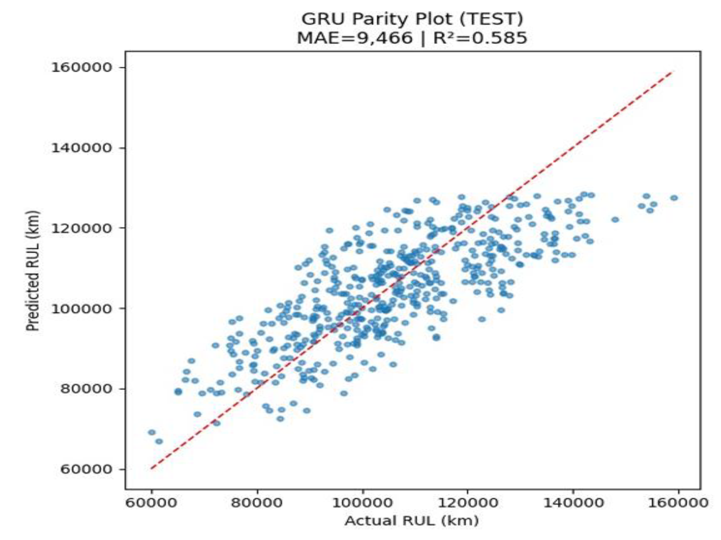
3.2.7.3. Gated Recurrent Unit (GRU) Pipeline
Figure 25 above displays the GRU model’s predicted vs actual Remaining Useful Life (RULₖₘ) values for electric vehicle traction motors, as assessed on the test dataset. The red dashed line represents a perfect prediction trajectory an ideal model would have all points along this diagonal. The GRU model yielded the Mean Absolute Error (MAE), 9,466 km, and R² Score: 0.585. The GRU network demonstrates strong predictive performance, with an R² value comparable to other top-performing models like the Random Forest and HGBR. While not outperforming the LSTM model, it still shows substantial generalization capability in time-series modelling. Key insights include moderate clustering around the ideal line, slight dispersion at higher RUL values, and temporal learning benefits.
4. Discussion of Results
With reference to Table A2 in the appendix, the traditional ensemble models (Random Forest, HGBR, LightGBM) and the LSTM/GRU models exhibit the best performance for RUL prediction in this comparison. They combine low error with relatively high R², indicating both accuracy and good variance explanation. The SVR and KNN also perform decently (errors ~9.0 km, R² ~0.56–0.58), suggesting that even simpler models can be effective when tuned well. On the other hand, complex deep models do not guarantee better results as seen in the basic Keras fully connected network underperformed, possibly due to insufficient sequence modelling or training issues. The CatBoost anomaly (high error and negative R²) might result from overfitting or difficulty with the data characteristics, showing that model choice and hyperparameter tuning are critical. These findings align with common observations in RUL literature: while deep learning methods hold promise for capturing nonlinear degradation patterns, well-tuned traditional models often provide strong benchmarks. The plot highlights that LSTM provided the best overall balance of error and R² (highest R² ~0.61 with error ≈9.1k km), edging out the Random Forest’s purely error-based advantage, and underscores the importance of evaluating models on multiple metrics for a comprehensive assessment of prognostic performance.
5. Conclusions
The main objective of this article is to develop and validate a multi-stage testing protocol for remanufacturing spent electric vehicle traction motors. The conclusion reached for the decision-making framework for remanufacturing spent electric vehicle traction motors is that the developed algorithm achieved moderate RUL prediction accuracy (highest R² ~0.61 with MAE ≈9.1k km), and the EDA confirmed that higher mechanical and thermal stresses significantly shorten motor lifespan. These analyses showed that motors with higher computed health indices indeed have longer expected lifetimes.
Appendix A

Table A1.
Electric Vehicle Traction Motor Data Set.
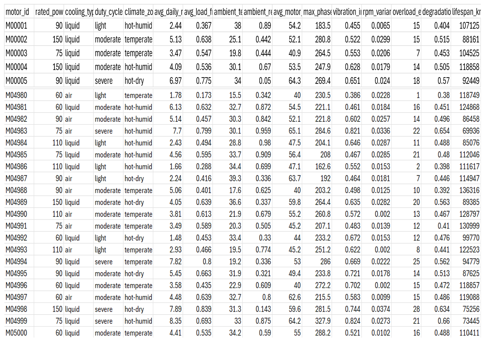 |
Table A2.
Comparison of ML & DL methods with evaluation metrics.
| ALGORITHMS | RMSE (km) | MAE (km) | R-Squared |
| Random Forest | 9,044 | 0.579 | |
| HistGBR | 9,055 | 0.579 | |
| SVR (RBF) | 9,190 | 0.556 | |
| KNN | 9,012 | 0.578 | |
| CatBoost | 14,269 | -0.119 | |
| LightGBM | 9,157 | 0.564 | |
| Keras | 14,133 | 11,359 | 0.295 |
| Long-Short-Term-Memory | 11,147 | 9,069 | 0.611 |
| GRU | 11,517 | 9,466 | 0.585 |
References
- Taheri F, Sauve G, Van Acker K. Circular economy strategies for permanent magnet motors in electric vehicles: Application of SWOT. Procedia CIRP, Elsevier B.V. 2024, 265–270.
- Mai Nguyen. Innovation in EVs seen denting copper demand growth potential. July 9, 202311:00 PM GMTUpdated July 9, 2023;
- VRW. The End-of-Life Vehicle Regulation is in its Final Approval Phase: What Next? 2025.
- VRW. China Issues National Standard for Reused ELV Parts. 2025.
- Xia Yu. MOFCOM’s New Notice on the Recycling of End-of-Life Motor Vehicles. 2024.
- Paulo-Guedes-Pinto. Why Remanufacturing Electric Motors is a Big Idea. 2025.
- Katona M, Orosz T. Circular Economy Aspects of Permanent Magnet Synchronous Reluctance Machine Design for Electric Vehicle Applications: A Review. Energies 17 2024. 17.
- Philip Akrofi Atitianti. ‘Greening’ Transportation: Electric Vehicles and Ghana’s sustainable mobility push. 2025.
- Botchway N, Calloway A, Aboagye Da Costa A, Lutterodt LL. Energy Laws and Regulations 2025—Ghana. 2024.
- Girbacia F, Daniel Voinea G. Multi-Method Statistical Analysis of Factors Influencing Predictive Maintenance of Electric Vehicle Fleets. 2025.
- Zhang, Y; Fang, L; Qi, Z; Deng, H. A Review of Remaining Useful Life Prediction Approaches for Mechanical Equipment. IEEE Sens J 2023, 23, 29991–30006. [Google Scholar] [CrossRef]
- Sayyad, S; Kumar, S; Bongale, A; Kamat, P; Patil, S; Kotecha, K. Data-Driven Remaining Useful Life Estimation for Milling Process: Sensors, Algorithms, Datasets, and Future Directions. IEEE Access 2021, 9, 110255–110286. [Google Scholar] [CrossRef]
- Sun J. Open Aircraft Performance Modeling Based on an Analysis of Aircraft Surveillance Data. TU Delft University 2019; 289.
- Sekhar JNC, Domathoti B, Santibanez Gonzalez EDR. Prediction of Battery Remaining Useful Life Using Machine Learning Algorithms. Sustainability (Switzerland) 2023; 15.
Figure 1.
Frequency Distribution of RUL.
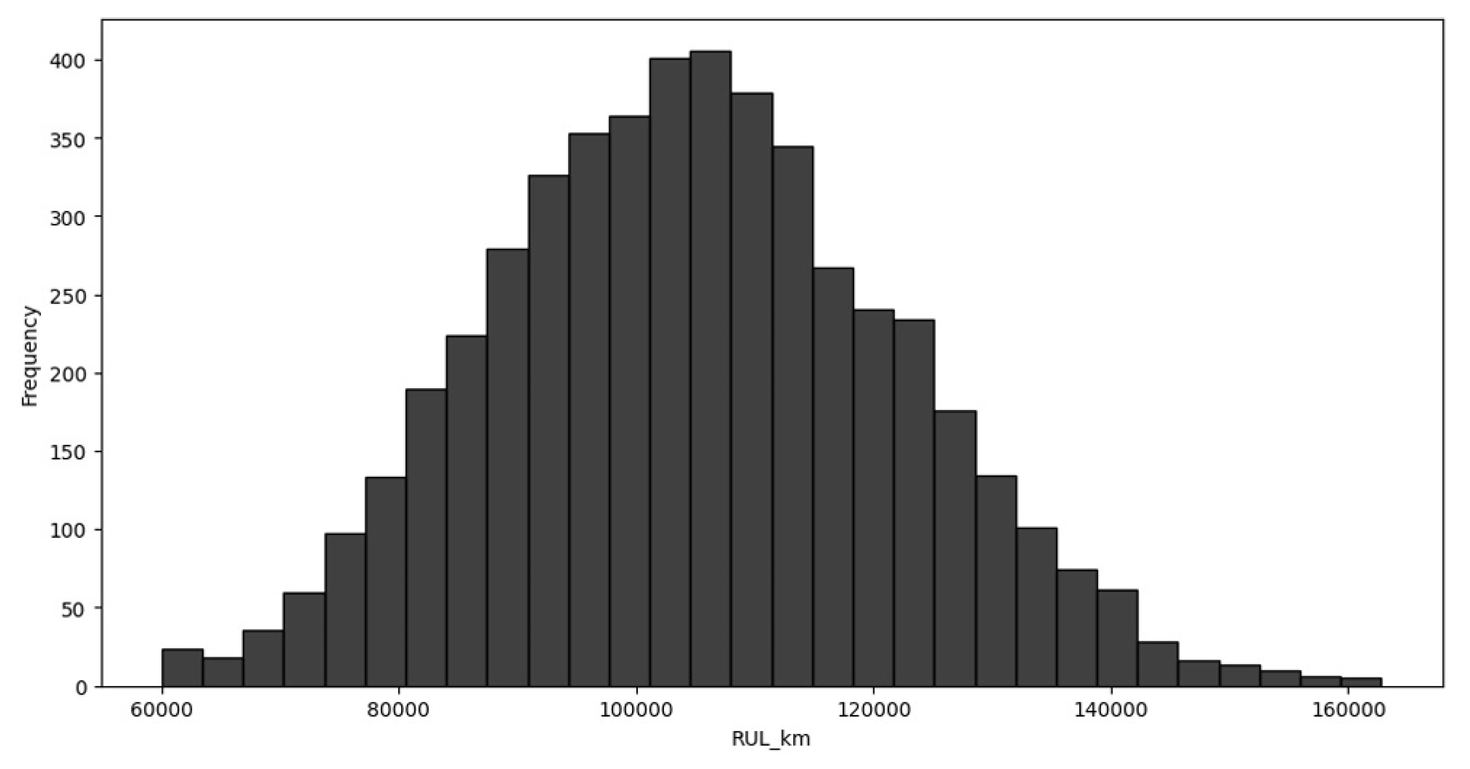
Figure 2.
Illustrates the Variation in the RUL of Traction Motors Across the Dataset.
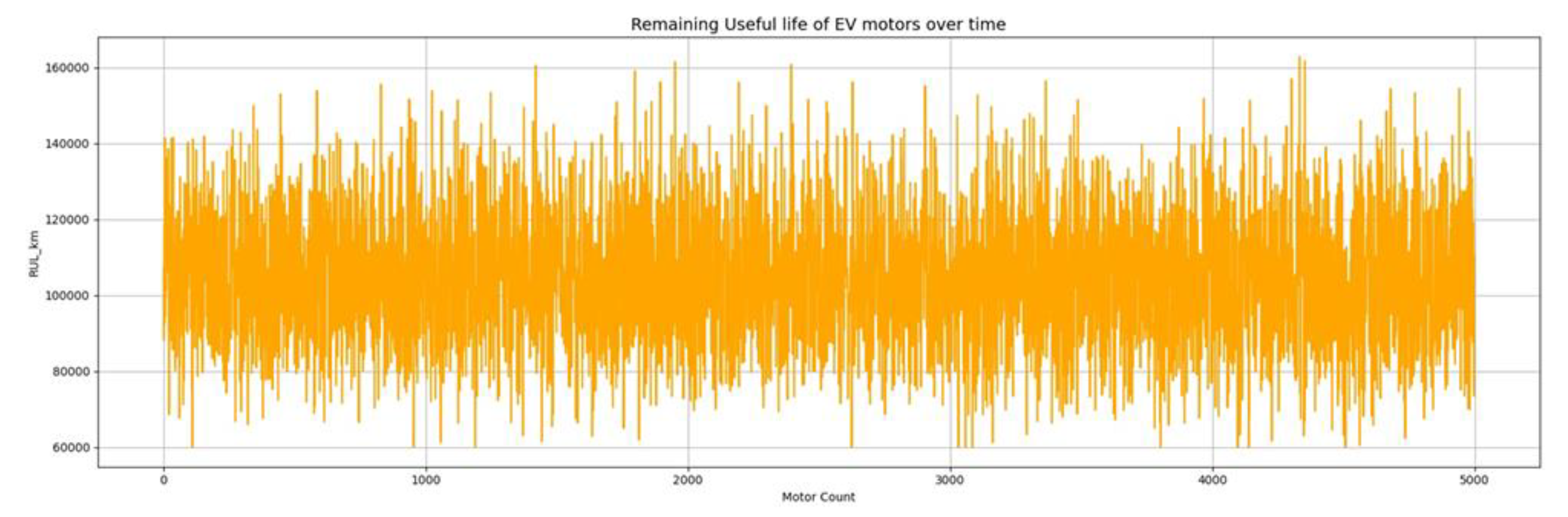
Figure 3.
The Spread and Variability of the RUL of Traction Motors.
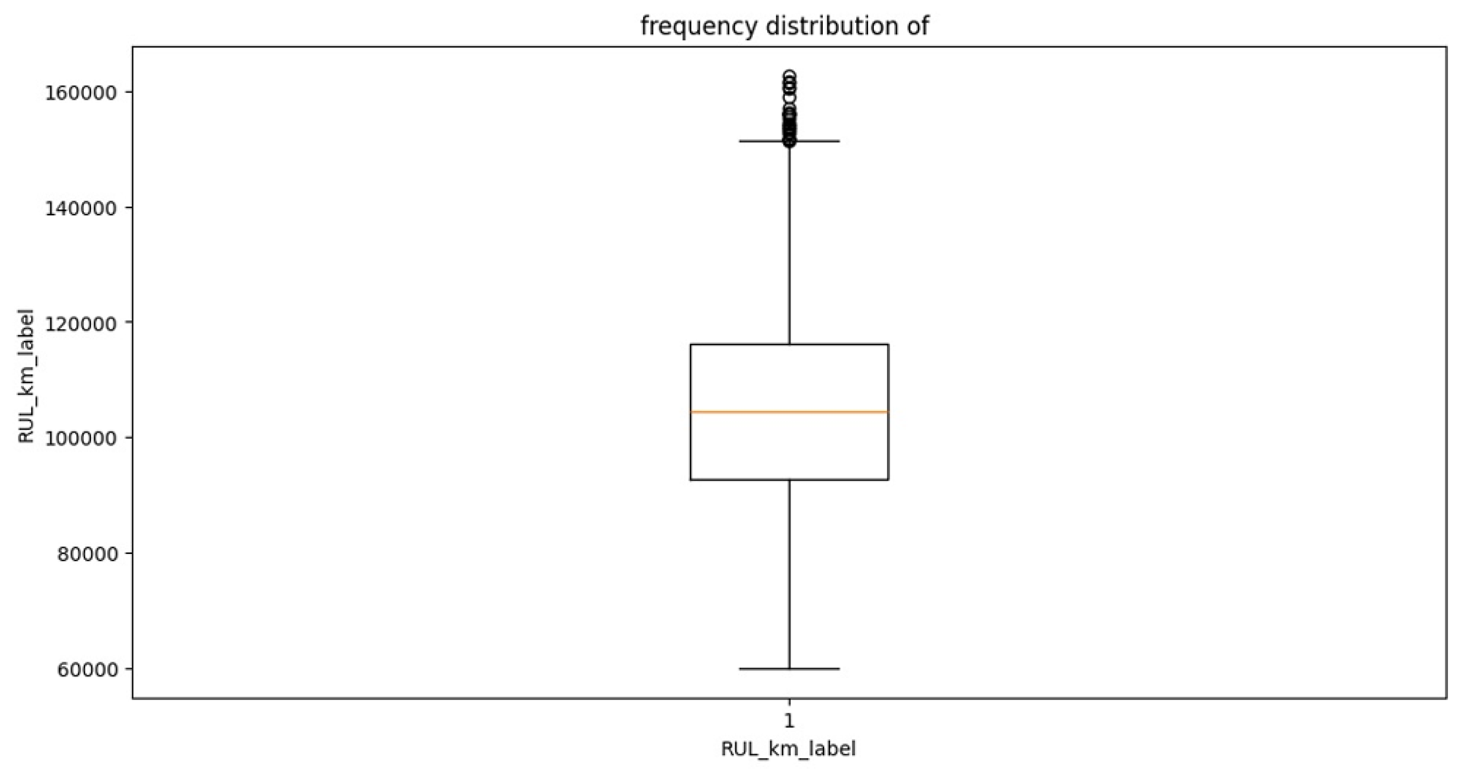
Figure 4.
The Pearson Correlation Heatmap.
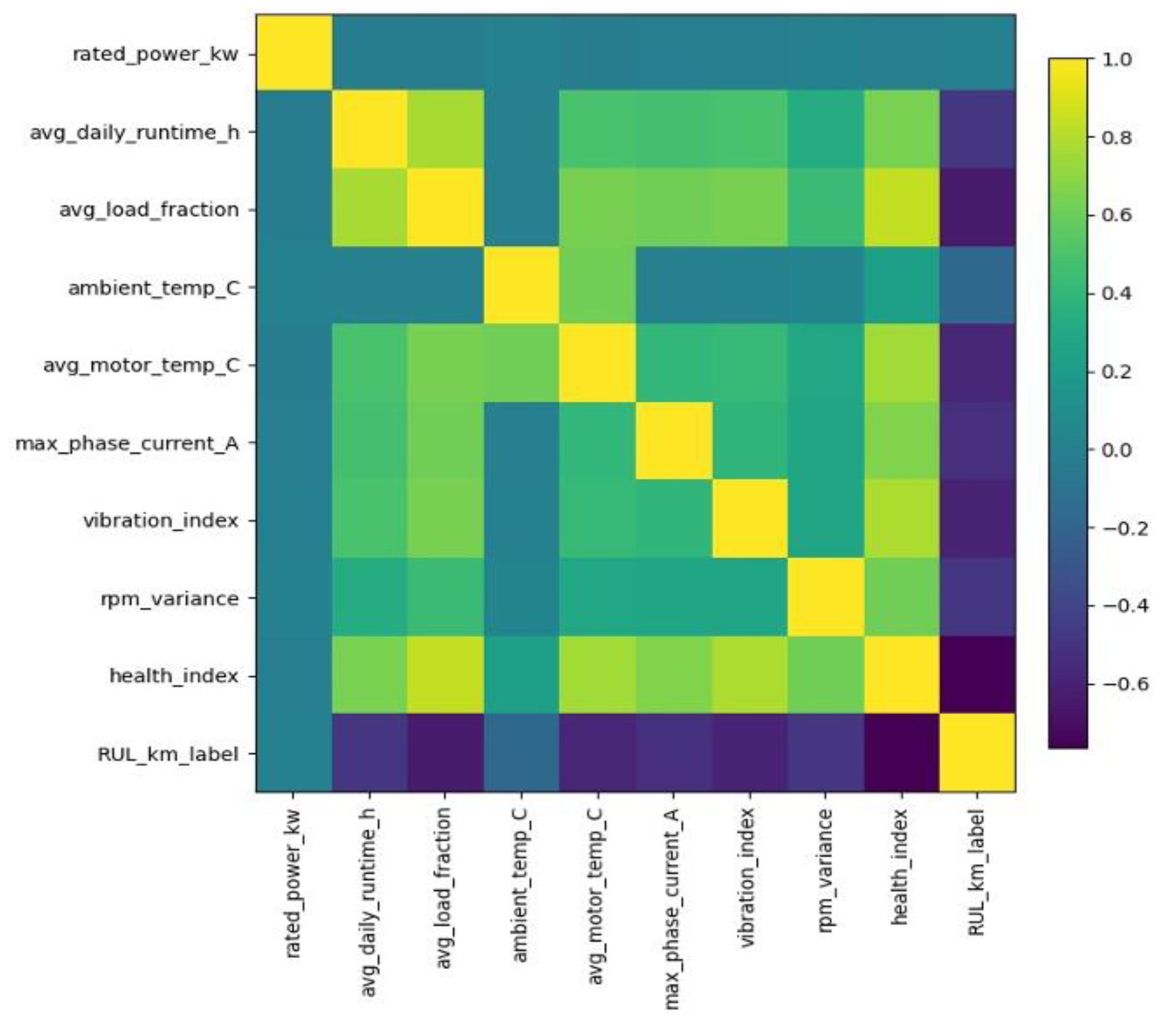
Figure 5.
Frequency Distribution.
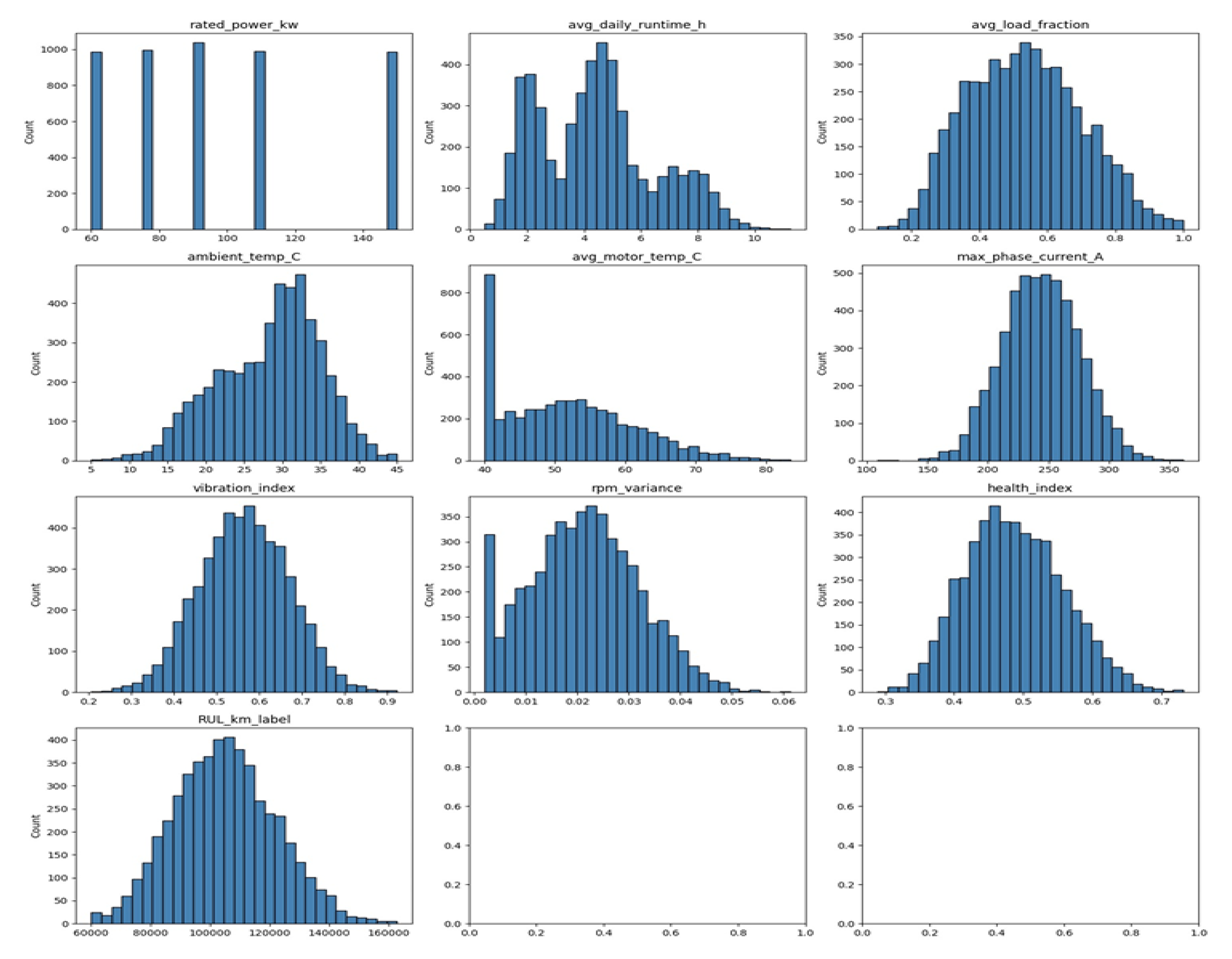
Figure 6.
Spread, Central Tendency, and Presence of Outliers.
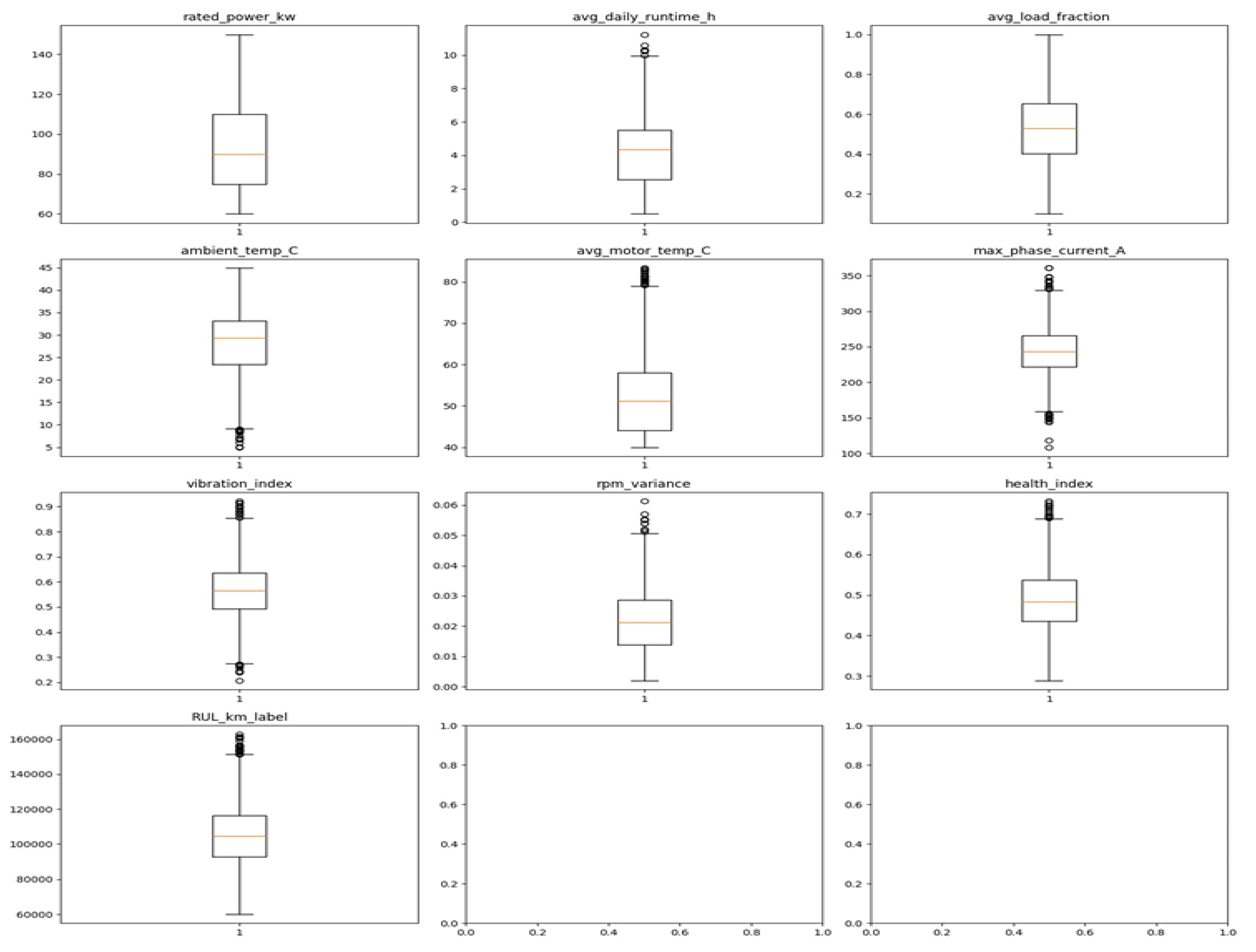
Figure 7.
Scatter Plots.
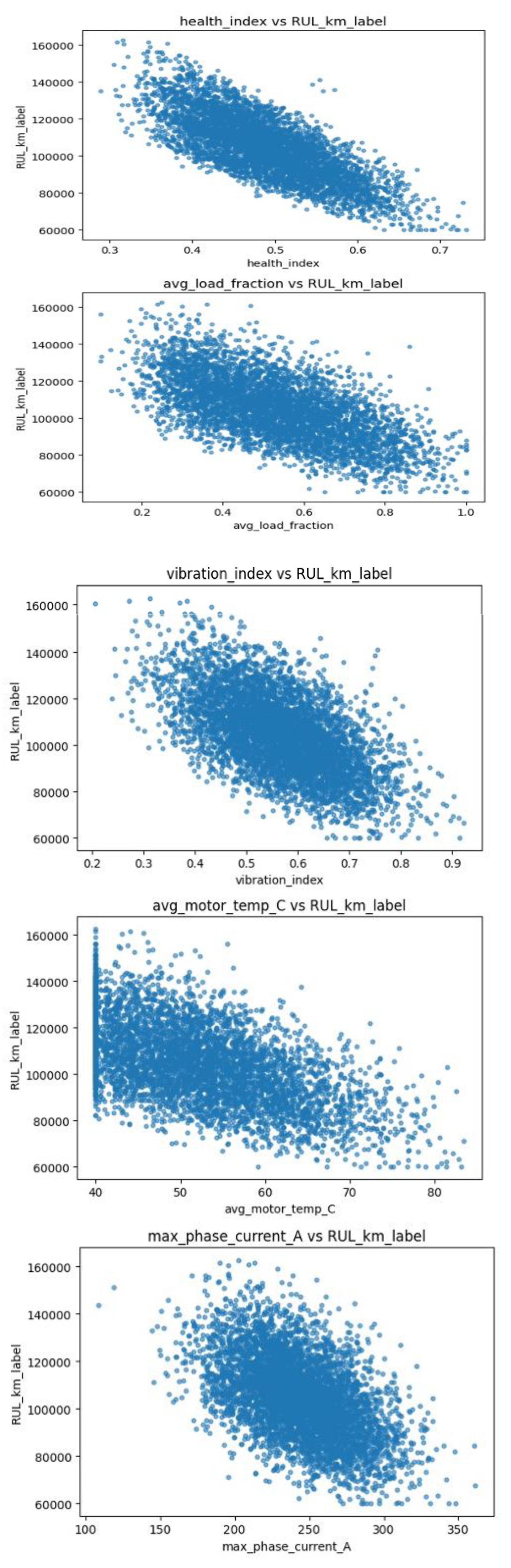
Figure 8.
Redefined Pearson Correlation Heatmap.
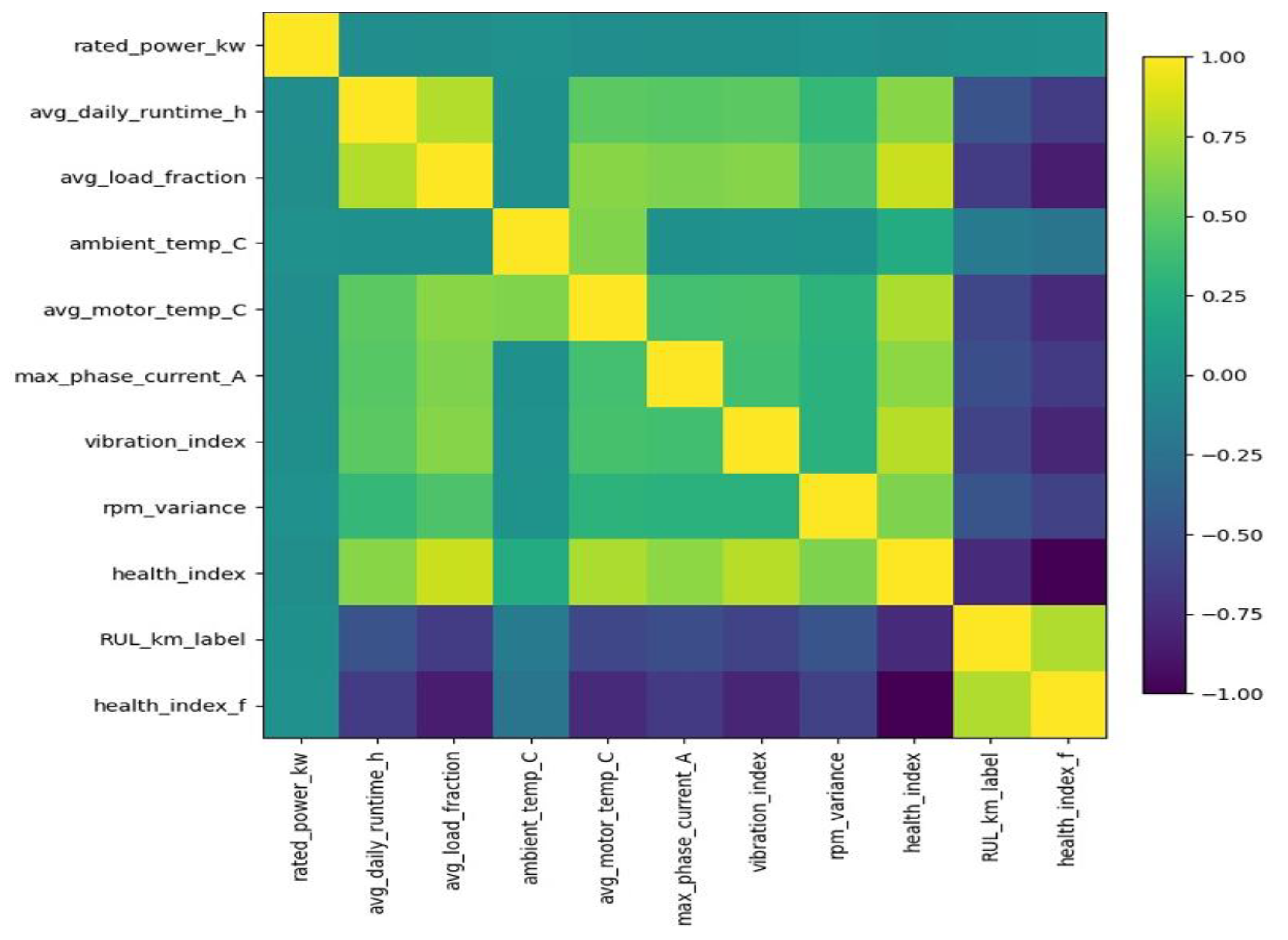
Figure 9.
Random Forest: Predicted vs Actual.
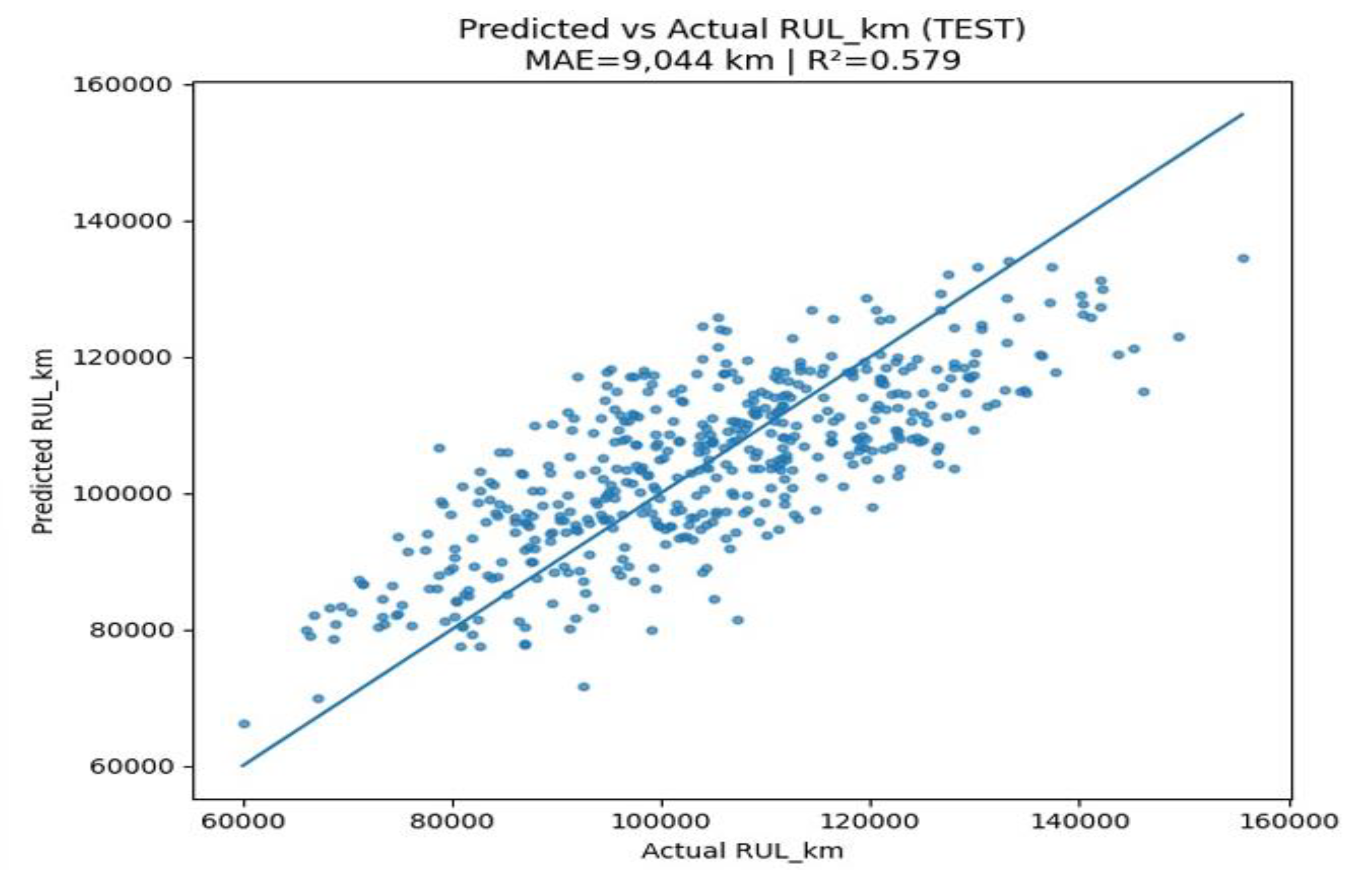
Figure 10.
Residual Distribution (Random Forest Model).
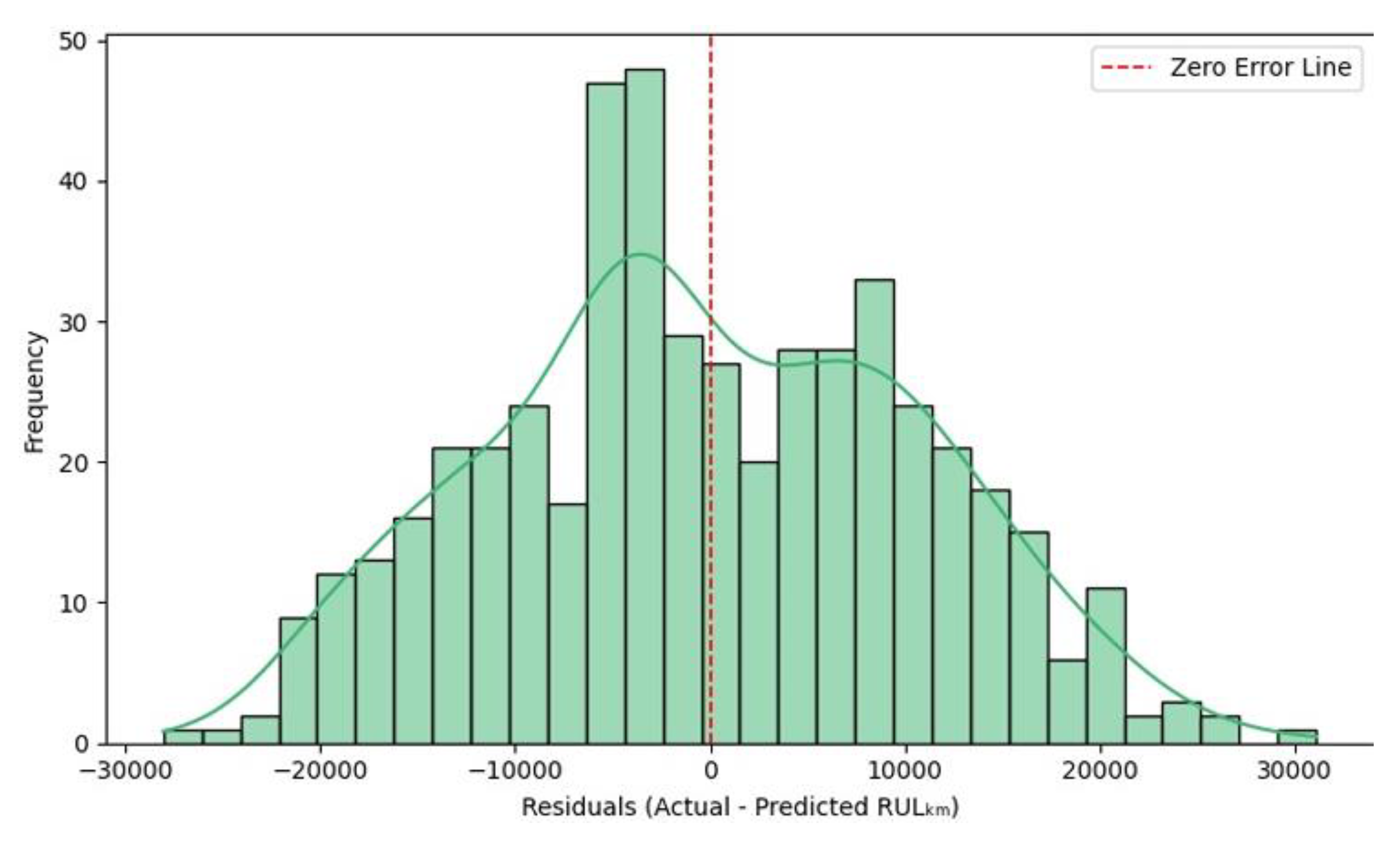
Figure 11.
HistGradient Boosting Regressor: Predicted vs Actual.
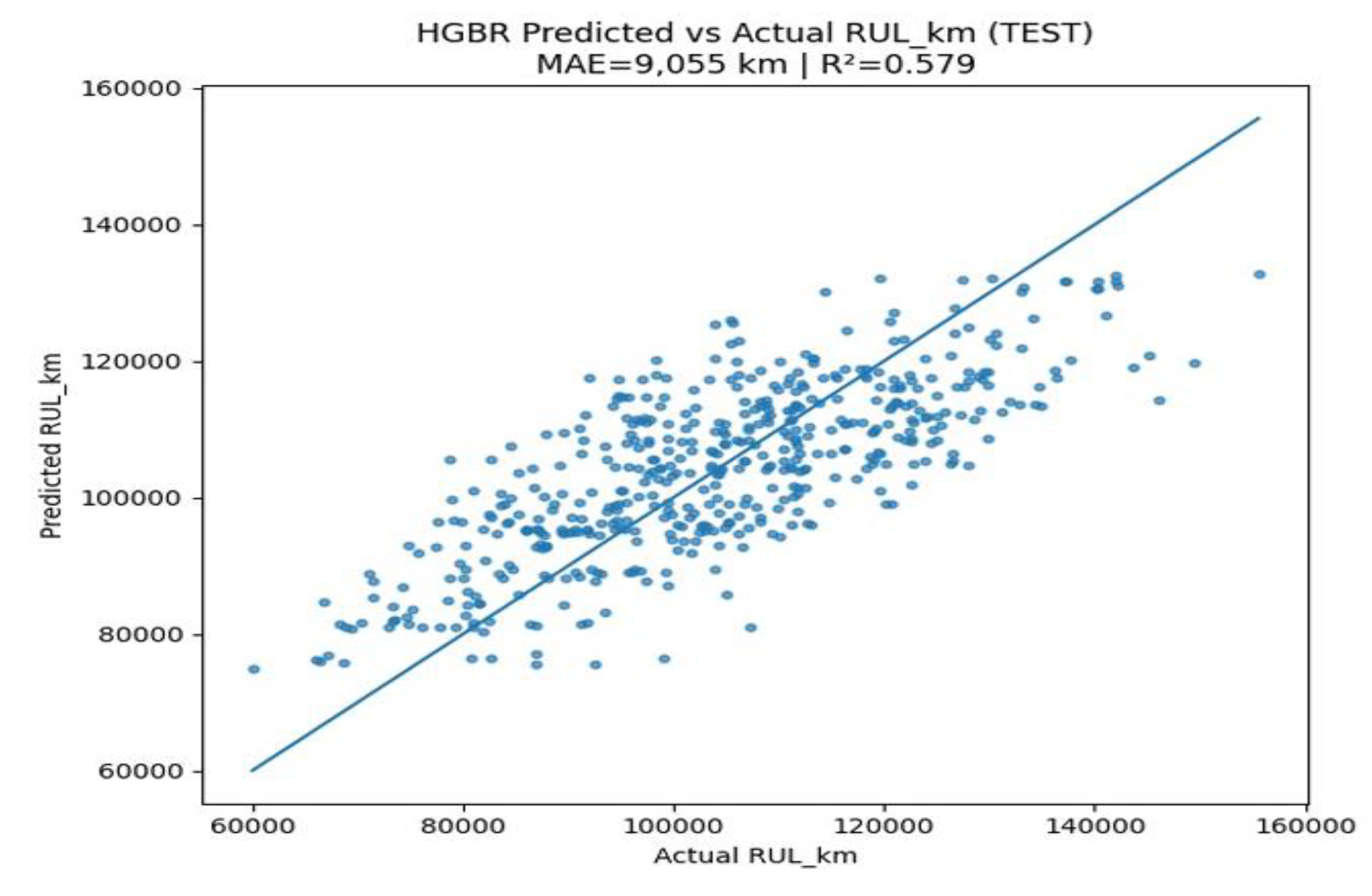
Figure 12.
Residual Distribution (HGBR Model).
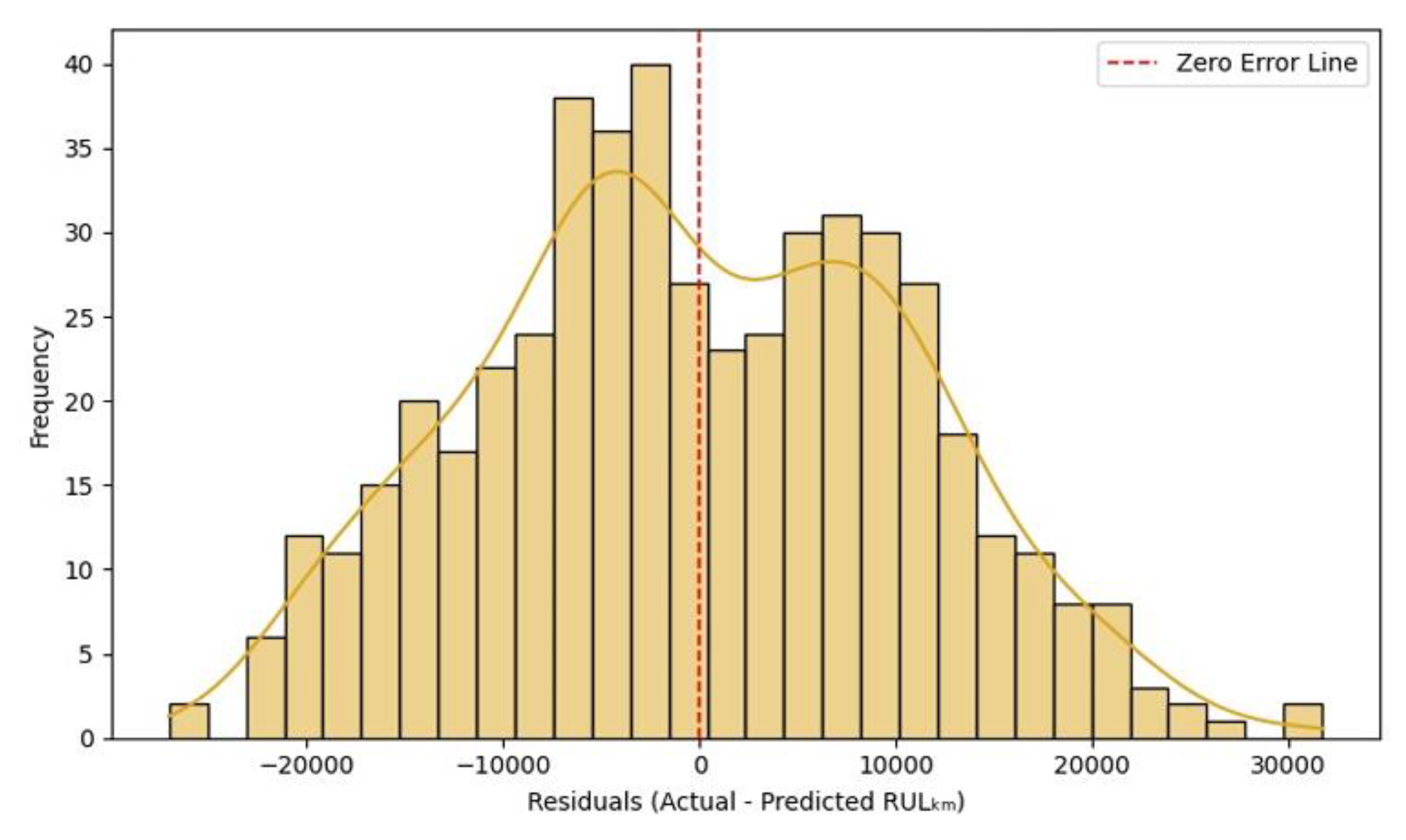
Figure 13.
SVR (RBF): Predicted vs Actual.
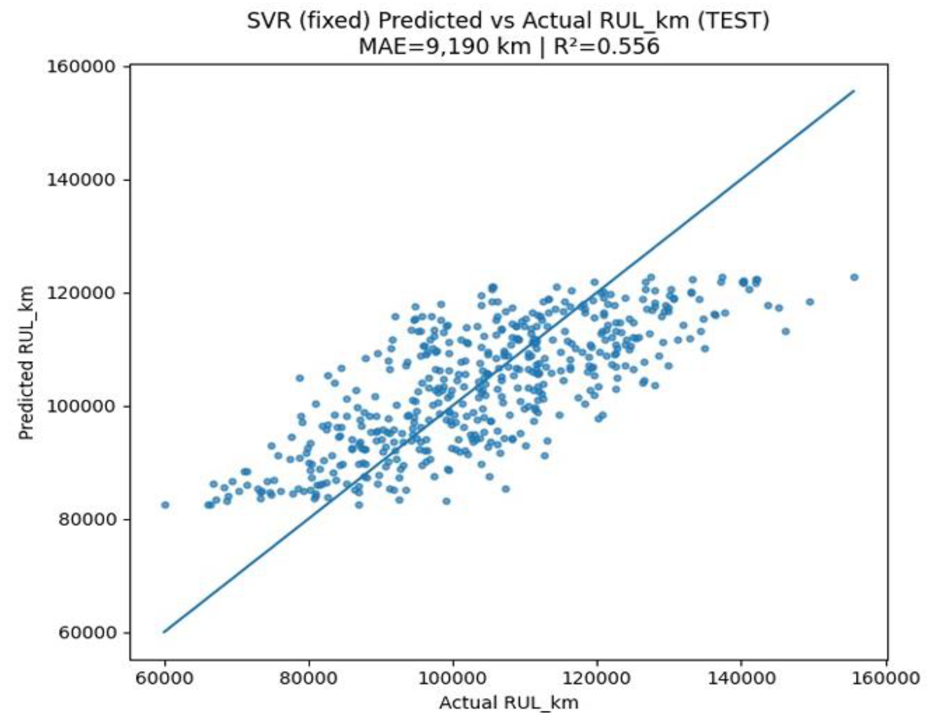
Figure 14.
Residual Distribution (SVR Model).
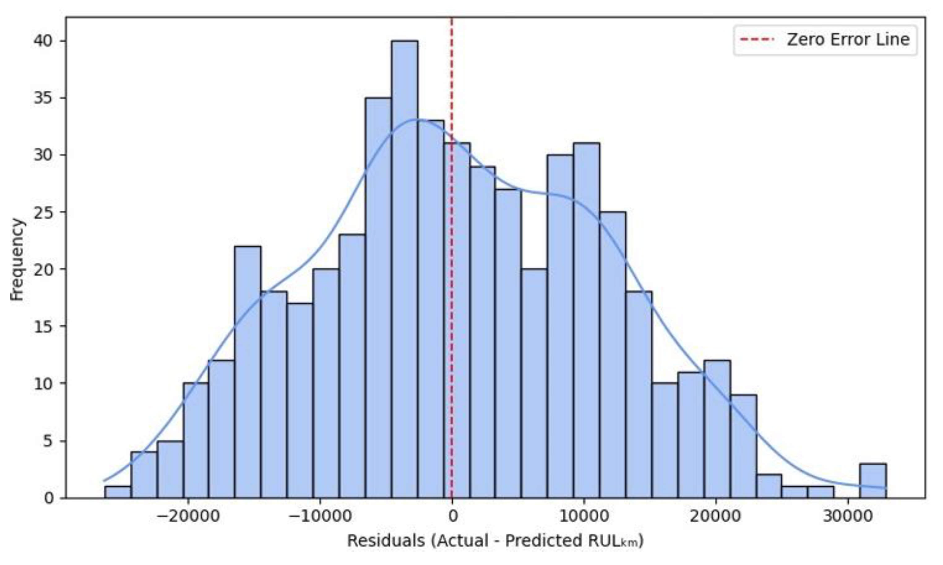
Figure 15.
KNN: Predicted vs Actual.
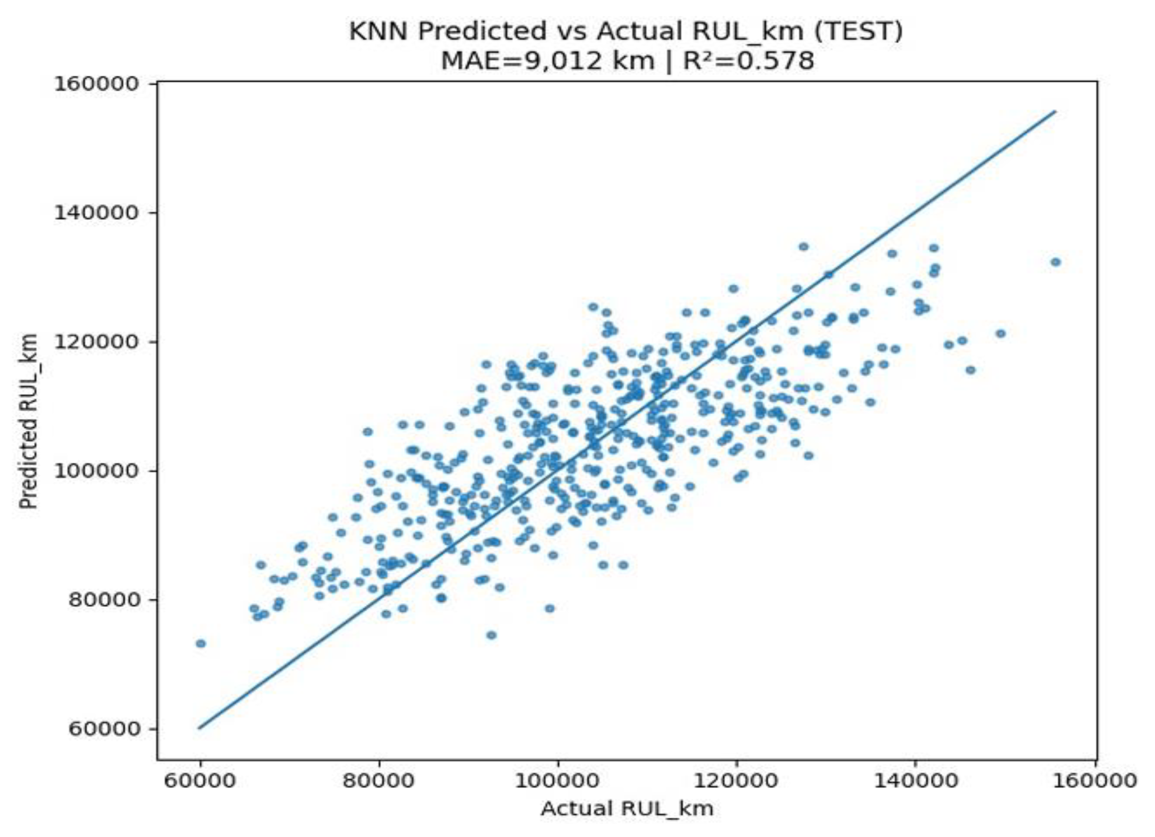
Figure 16.
Residual Distribution (KNN Model).
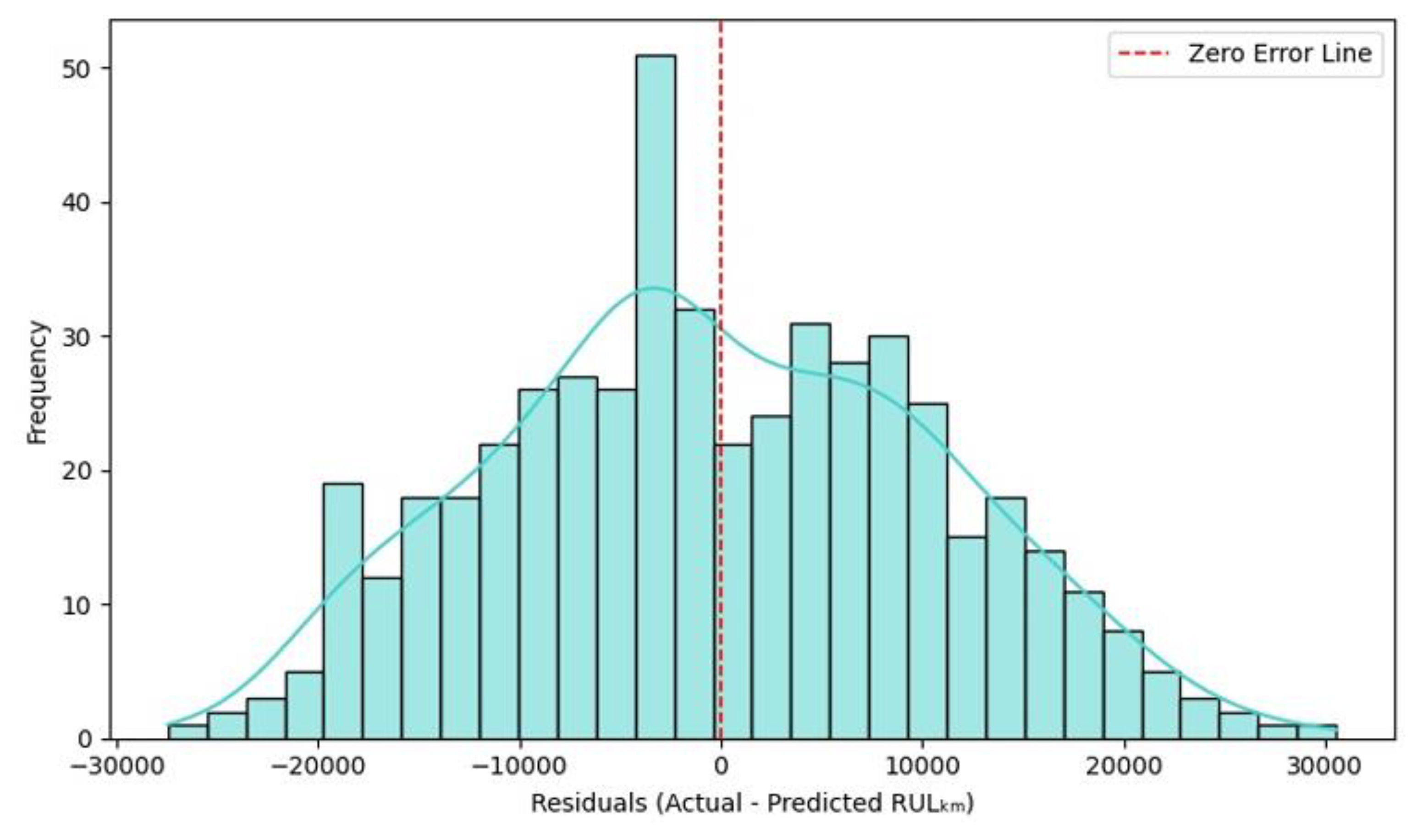
Figure 17.
CatBoost: Predicted vs Actual.
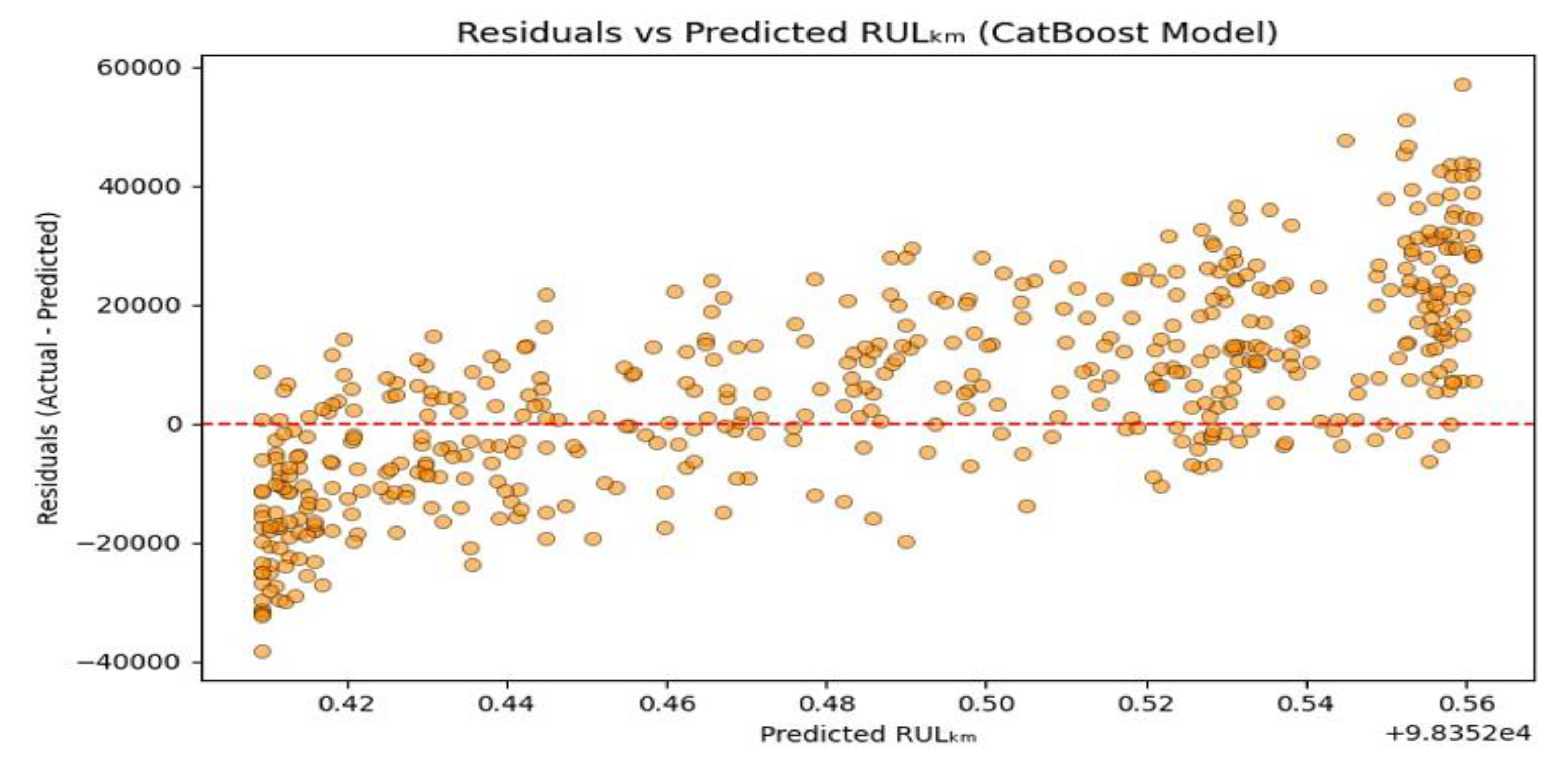
Figure 18.
Residual Distribution (CatBoost Model).
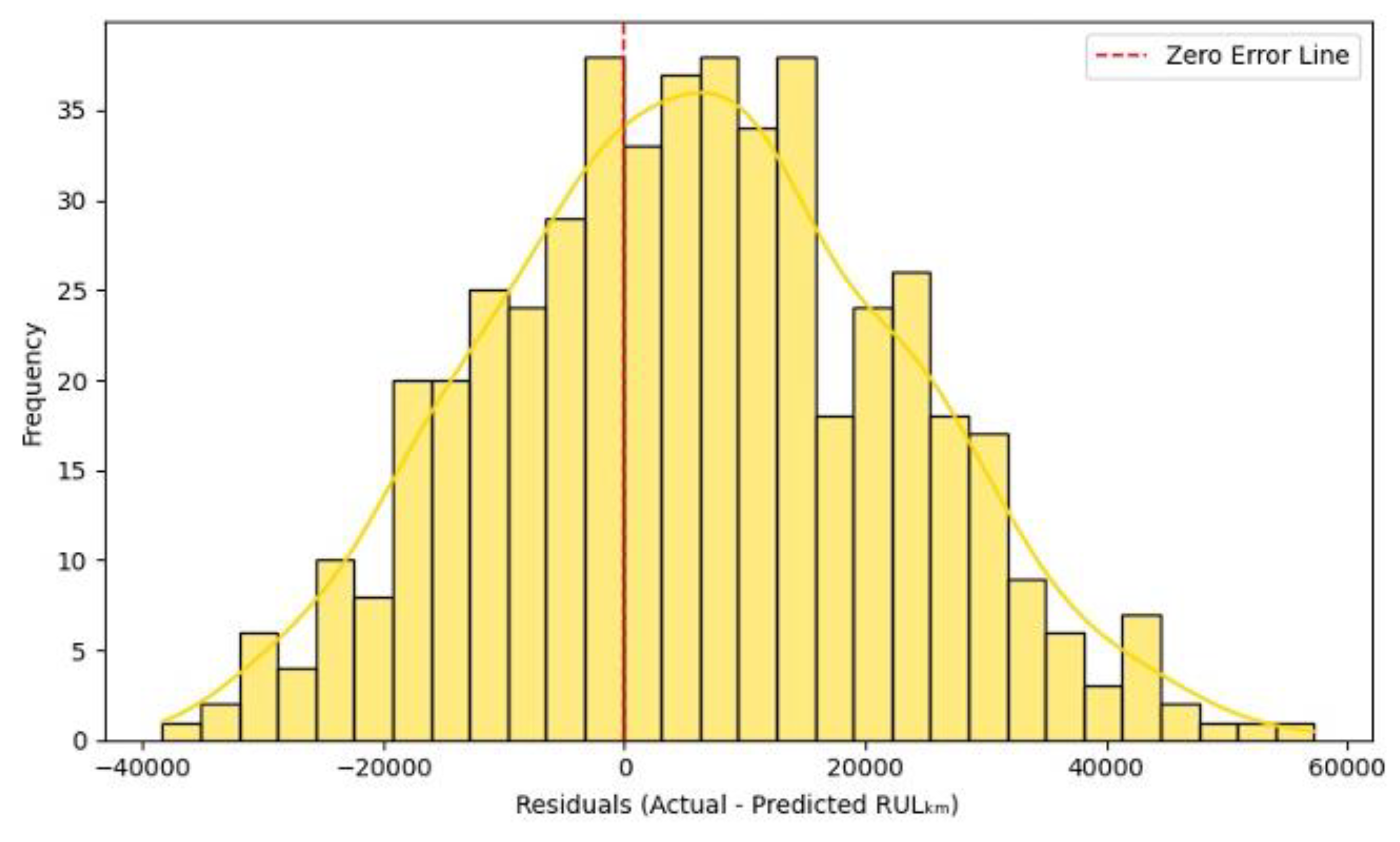
Figure 19.
LightGBM: Predicted vs Actual.
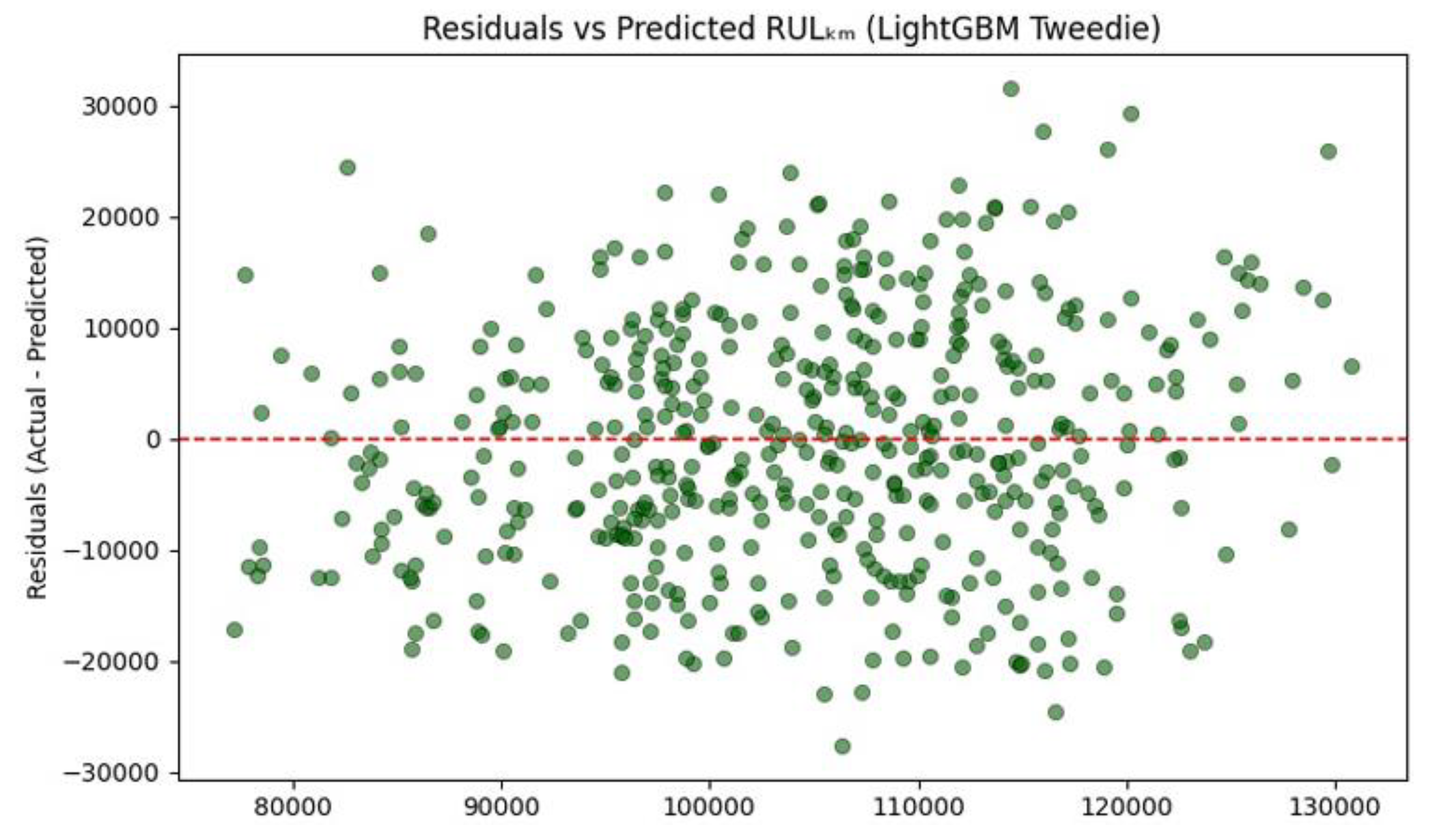
Figure 20.
Residual Distribution (LightGBM Tweedie Model).
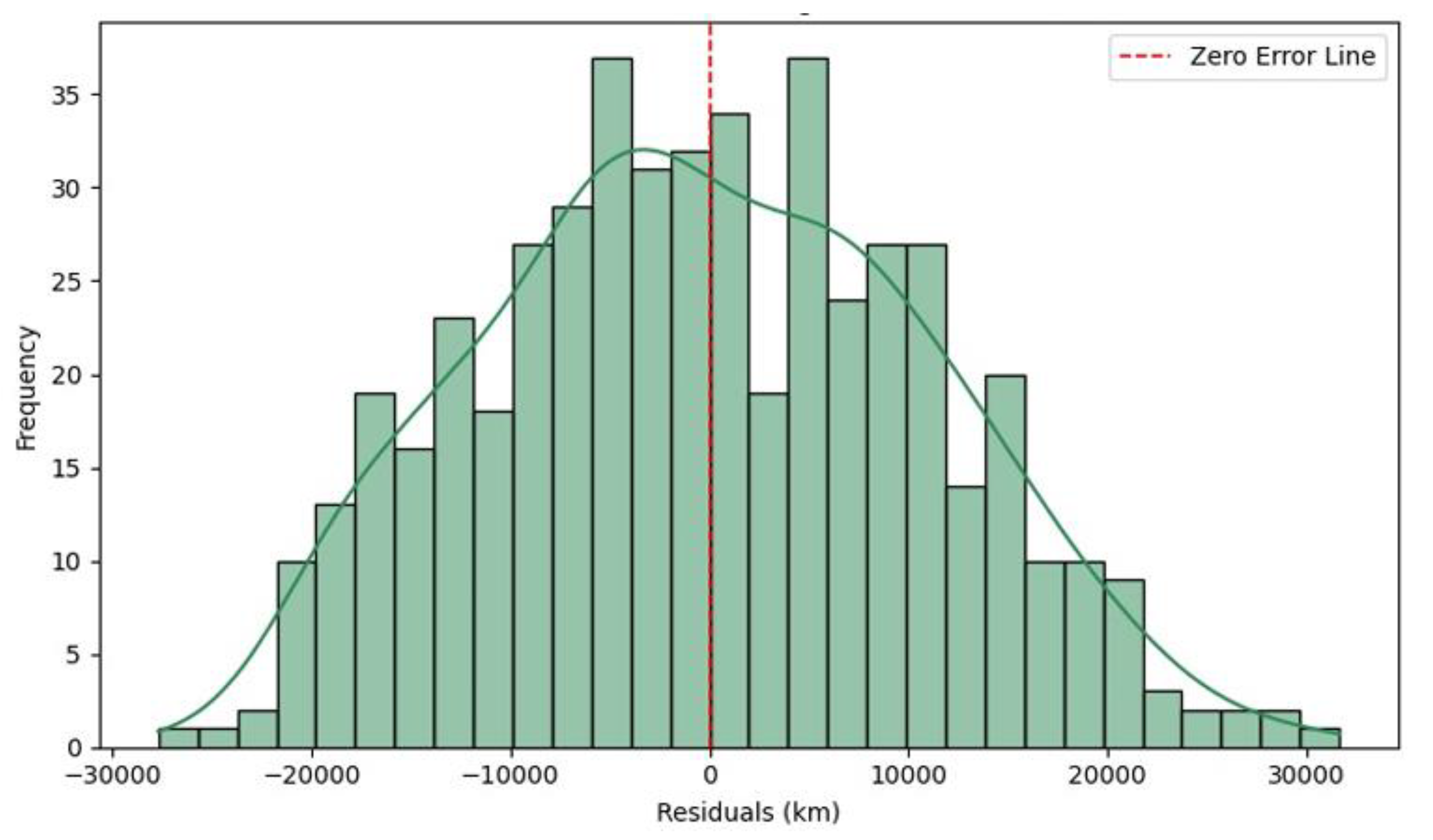
Figure 21.
Keras: Predicted vs Actual.
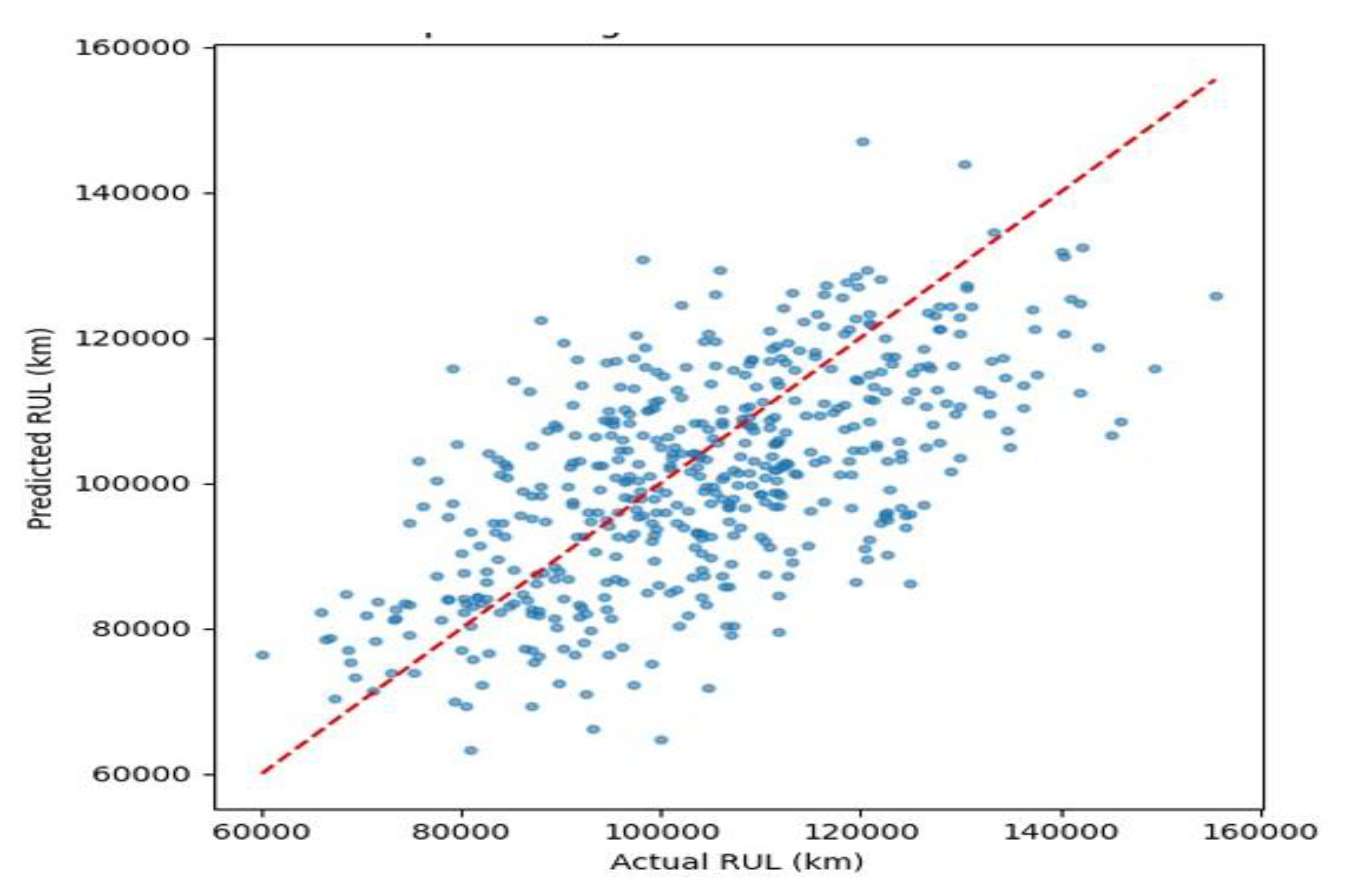
Figure 22.
Residual Distribution (DL Keras Model).
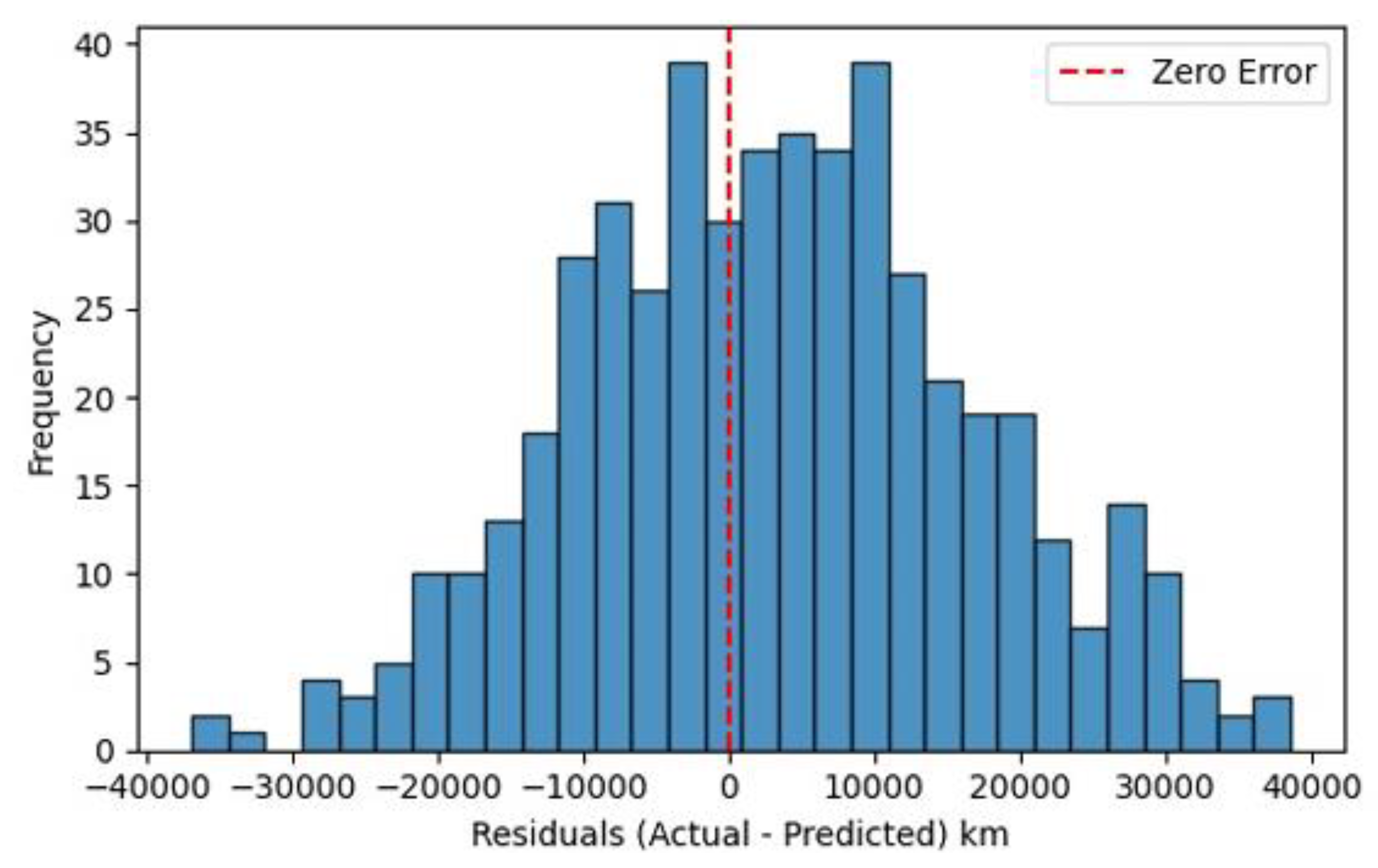
Figure 23.
LSTM: Predicted vs Actual.
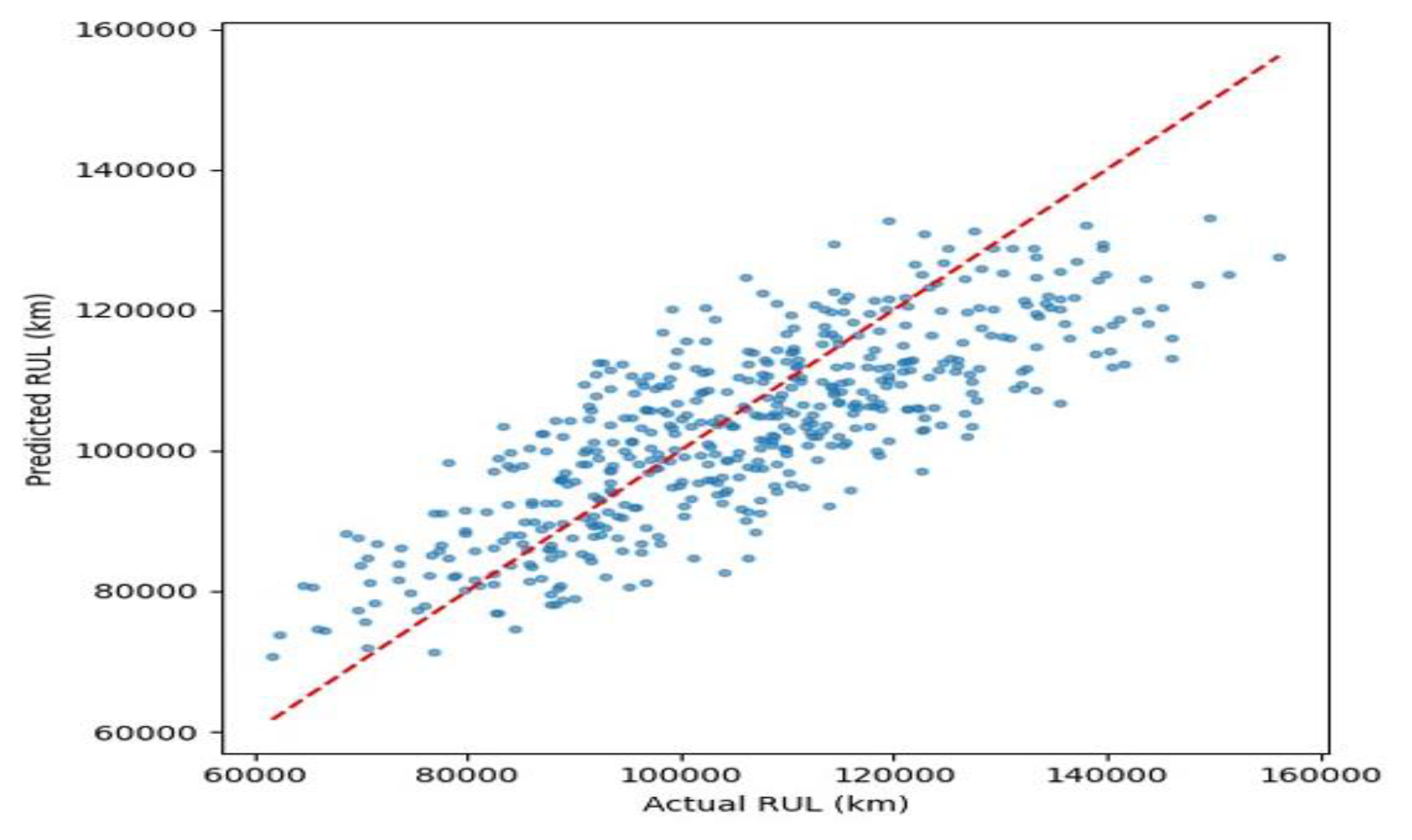
Figure 24.
Residual Distribution (DLLSTM Model).
Figure 25.
GRU: Predicted vs Actual.
Disclaimer/Publisher’s Note: The statements, opinions and data contained in all publications are solely those of the individual author(s) and contributor(s) and not of MDPI and/or the editor(s). MDPI and/or the editor(s) disclaim responsibility for any injury to people or property resulting from any ideas, methods, instructions or products referred to in the content. |
© 2026 by the authors. Licensee MDPI, Basel, Switzerland. This article is an open access article distributed under the terms and conditions of the Creative Commons Attribution (CC BY) license (http://creativecommons.org/licenses/by/4.0/).
Copyright: This open access article is published under a Creative Commons CC BY 4.0 license, which permit the free download, distribution, and reuse, provided that the author and preprint are cited in any reuse.


