0. Introduction
The conformal compactification of Minkowski space has long played a central role in both mathematical relativity and conformal field theory. In its standard realization, the compactified space is obtained as the projective null cone of a six-dimensional real vector space of signature
, and is often described, following Penrose, as the “Einstein universe” [
1]. Although this construction is classical and widely used, several geometric and conceptual aspects of the compactification and of its conformal infinity are still presented in a manner that can obscure their true structure. In particular, the topology of the compactified space, the role of the natural double cover, and the precise geometry of conformal infinity are sometimes treated in the literature in a way that leads to confusion or to oversimplified pictures, such as the ubiquitous but misleading “double cone at infinity”.
The first aim of this paper is to provide a detailed and explicit re-examination of the conformal compactification of Minkowski space within the framework of the null cone in
. The construction is carried out in a basis-independent manner whenever possible, with coordinates used only as a technical tool where they clarify the geometry. A central result is an explicit identification of the compactified Minkowski space
with the unitary group
by means of a diffeomorphism, which gives a clear matrix representation of points in the compactification. This identification goes back to work of Uhlmann [
2], who used the Cayley transform to relate hermitian
matrices to elements of
. Here, an explicit formula is derived that realizes this correspondence directly on the projective null cone and shows in detail how the Cayley transform fits into the general geometric picture.
A second main theme of the paper is the analysis of the full conformal group and its connected component acting on the compactified space. After recalling the standard embedding of Minkowski space into the null cone and the induced conformal structure on , several important Lie subgroups of are described explicitly in terms of their matrix representations. These include the Poincaré group, dilatations, conformal inversion, and special conformal transformations. Their action on and, in particular, on conformal infinity is analyzed in detail. It is shown that the action of on is transitive, but not effective, since the central element acts trivially on the projective null cone.
This observation leads naturally to the consideration of the double cover
of the compactified Minkowski space, obtained by quotienting the null cone by positive rescalings rather than by all nonzero real scalars. The resulting manifold can be identified with the Grassmannian of oriented null lines in
and is shown to be diffeomorphic to
. On
the action of
becomes effective, and two disjoint embeddings of Minkowski space are obtained, corresponding to two non-intersecting copies
and
. The remaining part,
, plays the role of a “doubled” conformal infinity. This point of view clarifies statements in the literature where
is directly identified with
(see, for example, [
1,
3]) and makes explicit the relationship between the simple compactification
and its double cover
.
A substantial part of the paper is devoted to a precise geometric description of conformal infinity itself. Instead of the frequently drawn “double null cone”, the conformal boundary of the double cover,
, is shown to be a squeezed torus, namely a horn-type Dupin cyclide, while the conformal infinity
of the simple compactification is identified with a needle cyclide. These identifications are obtained by an explicit analysis of the intersection of appropriate quadrics in
, followed by a careful projection to three-dimensional Euclidean space. Parametric representations are derived and used to produce graphical illustrations of the resulting surfaces, which make the global structure of conformal infinity transparent and highlight, in particular, the presence of additional two-sphere components that are suppressed in the usual double-cone picture (cf. [
4,
5,
6]).
The final sections place these constructions into a broader geometric context. First, five-dimensional constant-curvature spaces are embedded so that their common boundary is the compactified Minkowski space, and the interpretation of geodesics in these ambient spaces is discussed. Second, the entire theory is reformulated in a coordinate-free language, following the approach of Kopczyński and Woronowicz [
7]. In this formulation the conformal compactification, its double cover, the conformal structure on the tangent bundle, and the null geodesics of the Einstein universe are described purely in terms of the quadratic form
Q on a six-dimensional vector space and its isotropic subspaces. This geometric reformulation not only clarifies the role of the tautological bundle and its orthogonal complement over the projective null cone, but also provides a natural setting in which to understand the conformal structure as an equivalence class of scalar products on tangent spaces and to see how null geodesics depend only on the conformal class of the metric.
The paper is organized as follows.
Section 4 recalls the basic construction of the compactified Minkowski space as the projective null cone and introduces the identification with
as well as the embedding of Minkowski space by means of the map
and the Cayley transform. The conformal group
, its connected component
, and their important subgroups are then discussed, together with their action on
and on conformal infinity. The double cover
and its decomposition into two copies of Minkowski space and the doubled conformal infinity
are introduced and studied in detail, including the description of
as a horn cyclide and the corresponding structure of
. Subsequent sections address the embedding into five-dimensional constant-curvature spaces, the induced conformal structure and its relation to null geodesics, and finally the coordinate-free reformulation of the theory in terms of the projective null cone and its tautological and orthogonal bundles.
1. Definitions
We denote by
M the standard Minkowski space, that is
with coordinates
endowed with the quadratic form
Let
be
endowed with the quadratic form
defined by
We denote by
the 6–dimensional space
with coordinates
and endowed with the quadratic form
Let
be the null cone of
minus the origin:
and let
be the set of its generators, that is the set of straight lines through the origin in the directions nullifying
In other words
where, for
if and only if there exists a nonzero
such that
We denote by
the natural projection
Then with its projective topology, is a compact projective quadric. is called the compactified Minkowski space, denoted also by
A. Uhlmann [
2] used the Cayley transform to identify the compactified Minkowski space with the group
of complex unitary
matrices. The following proposition provides the identification of
with
in an explicit form.
Proposition 1.
For each the matrix
is unitary and depends only on the equivalence class of The map descends to a diffeomorphism from onto the unitary group
Proof. Let
. From the definition (
4) of
we have that
and
These two conditions are equivalent to
It follows, in particular, that
Therefore the right hand side of Eq. (
6) is well defined for all
, and is a smooth function of
A straightforward calculation gives us
where
is the
identity matrix. Taking into account the condition (
8) we deduce that, for
the matrix
is in
Notice that it follows from Eq. (
6) that for every
and
we have
therefore the function
is constant on the equivalence classes of the equivalence relation ∼ defining
and so it defines the map
from
to
We will now show that the map
is surjective.
Let
U be an arbitrary matrix in
. Since
it follows that
Let
c be one of the two (complex) square roots of
, so that
Since
we have
Then
is of determinant 1, i.e.
is in the group
, and we also have
Now, every element
of
can be uniquely written in the form
where
are complex numbers satisfying
which, by the way, gives us the well known topological identification of
with the sphere
. Defining
that is writing the complex numbers
as
one can verify that
, with
Therefore the map
from
to
is indeed surjective. Let us finally check the injectivity of the map
. Let
and
be in
, and suppose
We may assume that
and
as defined in (
8), are both equal to 1, otherwise one can rescale
X and
using property (
10) to make it so. In other words, we may assume:
Using simple algebra and taking into account Eqs. (
14) we find that the equality
leads to
which, together with
entails
From
it then immediately follows that
, therefore
□
2. Embedding of M into
Here we adapt the standard methods of Möbius geometry of Lie spheres, as discussed, for instance, in [
4] (Ch. 2, Eq. (2.6)). Consider the following smooth map between manifolds:
given by the formula:
The map
is evidently injective. Let
be the hyperplane in
defined by the formula
Lemma 1. The image of M in coincides with the intersection of the null cone with the hyperplane
Proof. It is clear that, for all
It also follows by a straightforward calculation that
thus
From Eq. (
17) we have that
is also in
Thus
is a subset of
To show that
let
be in
From
we get
But
so that, from
it follows that
Together with
it implies
or
and
It follows that
□
Remark 1. Eqs. (17) and (18) take a simpler form when, instead of orthogonal coordinates null coordinates are being used, as it is done e.g. in [6]. If we use these coordinates, and if we write X as then the quadratic form Q takes the form
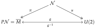
We now define the embedding
by
We thus have the following (commutative) diagram, where doubled arrow ends denote surjections.
2.1. The Conformal Infinity
Now, if and we can set . Then so that X and define the same point in But now It follows that the points of which are not in the image of M are equivalence classes of those for which These points define the conformal infinity. Another method of defining the same set is described in the next section
2.2. Embedding via the Cayley Transform
Denote by
the set of all complex hermitian
matrices.
is a real vector space of dimension
For
let
be defined as
Then is an isomorphism of real vector spaces M and
For every
let
denote the matrix
Then is in , and the map is injective. The map is called the Cayley transform. Composing we get an embedding of M into , but the following proposition shows that it is the same as
Proposition 2. The following diagram is commutative:
Proof. Since all the maps in the diagram are given explicitly, checking of the commutativity is a matter of a simple algebra. □
2.3. Conformal Infinity Within
Suppose we want to invert the Cayley transform
and express
A in terms of
We multiply both sides by
- it does not matter which side, since
A and
U commute. We get, after regrouping the terms:
We notice that we can express
A in terms of
U if and only if
is invertible (i.e. iff
U does not have 1 as one of its eigenvalues). The set of those matrices for which
is not in the image
We denote this set by
and call it the
conformal infinity. This is not a one-point compactification. We add to
a whole (closed) “cap” - a three -dimensional manifold
Remark 2. is not exactly a smooth manifold. As we will see it has a singular point, a `corner’. Usually it is referred in the literature as `the double cone at infinity’, but it is not a double cone at all (Cf. [5]). It is a Dupin cyclide - Cf. (Section 6.5).
3. Action of the Conformal Group
Let
G be the diagonal matrix
so that for
we have
The group
is defined as the group of all real
matrices
L satisfying
It is evident that, for every if X is in , i.e. if and , then also is in Moreover, L maps equivalence classes of ∼ into equivalence classes, therefore the action of on descends to its action on We define as the subgroup of consisting of matrices of determinant
3.1. The Group
In order to separate four space-time coordinates from additional two coordinates we have chosen the signature of
Q as
In this subsection it will be convenient to choose the signature
the two signatures being equivalent by permutation of coordinates. Formally it can be achieved by switching the coordinates
and
, that is by a similarity transformation
,
where
R is the matrix
Notice that
and that
is equivalent to
Now it is convenient to write
in a block matrix form, using matrices
of respective dimensions
:
Then the condition
translates to:
where we denoted by 1 the identity matrices of appropriate dimensions. In particular we have
which entails
and
Therefore either
or
Similarly, either
or
It can be shown (Cf. Refs. [
8,
9]) that, for
,
if and only if
We define
Then (Cf. [
10] p. 107)
is a connected subgroup (the connected component of identity) of
Proposition 3. The action of on the compactified Minkowski space is transitive.
Proof. Let and be any two points in Let us choose the representatives of the equivalence classes so that That means and The group acts transitively on the sphere therefore we can choose an orthogonal rotation from acting on the variables , and leaving the variables fixed, that transforms into Similarly the group acts transitively on the sphere therefore we can choose an orthogonal rotation from acting on the variables , and leaving the variables fixed, that transforms into The composition of these two transformations is in and maps X to □
Remark 3. Notice that the transformation is in and acts on as the identity map. Thus the action of on is not an effective action.
4. The Double Cover of
For
we define the equivalence relation
as
Definition 1. We will denote by the canonical projection
We denote by
the equivalence classes of this relation. Notice that while
we have
In fact each equivalence class of ∼ contains two equivalence classes of ≈. The projective space
is known as the Grassmannian of null lines in
We define
i.e. as the Grassmannian of
oriented null lines in
Proposition 4. is diffeomorphic to
Proof. Each equivalence class has now a unique representative X with Namely, if is arbitrary, then is this representative. Now, if , we define , , and then and . Conversely, any such pair of defines with □
Remark 4. Penrose and Rindler, in their classic monograph [1] (p. 298-299) state (Eq. (9.2.1)) that (denoted there ) is homeomorphic to For a non-expert reader this can be somewhat confusing. As we have seen can be identified with , which is a double cover of In Ref. [3] is denoted and called “the Einstein space”.
The action of
on
is defined the same way as for
We define
Proposition 5. The action of on is transitive.
Proof. The proof goes exactly the same way as for □
5. Important Subgroups of
In Eq. (
17) we have defined the embedding
of
M into
We will use this map to identify important Lie subgroups of
(and discrete transformations in
)
5.1. Translation Subgroup
We start with translations where
We have
where
is the scalar product of vectors in
and
Thus
or
But we want the transformation to be linear in
X. The trick is to multiply the right hand side by
We get this way the desired formula:
The transformation
is now implemented by the following matrix written in a block matrix form:
where
or explicitly:
One can easily check (for instance using a computer algebra software) that
and that
5.2. Lorentz Rotations Subgroup
For any Lorentz rotation
we have
therefore the way the Lorentz rotations are embedded in
(using our definition of
G) is evident. We simply set, using block matrix form,
5.3. Dilation Subgroup
This time we choose a different way. There is a natural subgroup of
similar to the Lorentz rotations case, but putting a "Lorentz rotation" in the lower right corner. This one-parameter Abelian subgroup is defined as follows:
where
Proposition 6.
For we have
Therefore the matrices implement dilations of the Minkowski space.
Proof. For
we have
where
Let
. Then
where
Now
Using also the definitions of
and
we obtain
□
5.4. The Conformal Inversion
Conformal inversion is defined in
M as the map
We assume that x is dimensionless, otherwise we would have to define it as where R is some "radius". Also notice that on M the transformation is singular on the null cone at the origin Under conformal inversion the null cone is mapped into a set of points at the conformal infinity of How? It will be clear after we derive the matrix representation of the conformal inversion, which we will do right now.
Assuming
and with
consider the following simple calculation:
But the end result is the same as acting on
with the following matrix
from the group
:
and then multiplying the resulting vector by
which is inessential when projecting on
using the projection
In other words conformal inversion is implemented on
by the reflection in the variable
Notice that
so
is in
but not in
Finally let us address the question of the image of the null cone at the origin by the conformal inversion. It follows from Eq. (
53) that this image is the `double null cone at infinity’:
But that is not yet the whole conformal infinity. What remains is the set
which is homeomorphic to the sphere
It is this sphere that connects the lower and upper branches of the null cone at infinity, and makes the conformal infinity into a compact set - Cf.
Figure 2. Many published papers on the subject omit this two-sphere and incorrectly identify the conformal infinity with the `double null cone’, as e.g. in [
6] (p. 263).
5.5. Special Conformal Transformations
This four-parameter Abelian subgroup of
is defined as:
The matrices representing
are similar to those representing
since the bracketing of any matrix
A with
results only in changing signs of the elements
in the fifth row and
in the fifth column, the element
changes sign twice, so it stays unaltered. Thus we have:
It is easy to get the action of the special conformal transformations on
From the definition we have
which simplifies to
Evidently, for a given the points x for which are transformed onto points in the conformal infinity.
5.6. Conformal Structure
Let
p be a point in
, and let
be a vector tangent to
at
A vector tangent at
p to
is a vector tangent to a smooth curve
such that
We will write it as
We will use now one of the intuitively clear important properties of projective manifolds, such as . Namely, given any there always exists a smooth curve defined for s in a neighborhood of , such that and We say that is a (local) lift of through X.
Of course such a lift is not unique. If
is any smooth function such that
then, locally,
is another lift of
through
In fact any two lifts of
through
X are related that way.
Now, in coordinates,
is described as a function
with
It is convenient to use the notation
for the scalar product
in
Since
is a null vector, we have
Taking the derivative with respect to
s at
we find that
In other words is perpendicular to
Let now
be any two tangent vectors at
and let
be two curves through
p such that
Let
and
be the coordinate expressions of lifts of
and
through the same
We define the scalar product of tangent vectors by the formula
For this definition to make sense we must show that the scalar product defined in this way does not depend on the choice of lifts through
To this end suppose
are two other lifts. Differentiating with respect to
s at
we get
Now, taking into account the fact that
and
we immediately find that
therefore the scalar product
is indeed well defined. It is now immediate that for any
,
, we have
Therefore what is defined at p is not a scalar product, but an equivalence class of scalar products, where two scalar products are considered to be equivalent if they are proportional, with a proportionality constant that is strictly positive.
We say that we have defined this way a conformal structure on To give a Riemannian (or pseudo-Riemannian) structure on a manifold is to specify a scalar product at each tangent space. When only a class of proportional scalar products is defined, we call it a conformal structure.
5.7. Calculating the Conformal Structure of Explicitly
The map
defined in Eq. (
17) defines a coordinate system on an open dense subset of
. We will now derive the expression of the
invariant conformal structure in the domain of this coordinate chart. Let
p be a point in this domain, and let
be the point in the Minkowski space
for which
So
p is represented by
Of course
p can be represented as well by
but let us concentrate on
In coordinates a tangent vector at
x has coordinates
. Let
be a curve through
In coordinates it is represented by a curve
Then
defined by
is a lift of
to
Differentiating the last equation with respect to
s at
and taking into account the explicit form of
we obtain
Let us calculate an explicit formula for
. With
from Eq. (
71) we easily get
the other two terms cancel each other.
In other words: the invariant conformal structure on in a local chart of Minkowski space coordinates consists of scalar products proportional to the standard Minkowski space scalar product.
6. The Case of the Double Covering Compactification
Here we will find out what needs to be changed and how if we replace the simple compactification with its double cover
6.1. The Action of Becomes Effective
If G is a group acting on a set we say that the action is effective (resp. free) if, for and for all (resp. for some) implies that g is the identity element of In other words the action is effective if every different from the identity element of G does something nontrivial to something (to some element of M), and free if every different from the identity element of G does something nontrivial to everything (to every point of M). Thus every free action is effective, but there exist actions which are effective but not free.
Consider the matrix
, which is in
It acts on every
replacing it with
. But
X and
are in the same equivalence class of ∼ so
- they define the same point of
. The matrix
does nothing to all points of
- the action of the group
on
is not effective - we are losing information. But, for
X and
define two different points of
Therefore
acts nontrivially on
In fact, we have an effective action of
on
1
6.2. The two Embeddings .
Eq. (
17) defines the embedding of
M into
:
Replacing
x by
and taking into account the fact that
we obtain another embedding, we call it
:
while the first embedding we call
Remark 5. We could as well define It would also work. Which definition will prove to be more convenient will be seen only after a physical interpretation will be given to these constructions. As it is above the transformation implements space and time inversion on M.
6.3. The Doubled Conformal Infinity
and are two nonintersecting copies of M embedded in Their union forms an open dense set in
Let us define
where
is as in the Definition 1,
Section 4. Then
is a sum of three disjoint sets
We have two copies of M: and , and the doubled conformal infinity
The matrix
is in
and it maps
into
and equivalence classes of ≈ into equivalence classes. Therefore it defines a unique mapping
such that:
We evidently have
Remark 6. The action of ι on is free. Or more precisely: the action of the two-element group on is free. The two-element group is isomorphic to the group - the additive group of integers modulo 2. It acts freely on can be identified with the quotient
We will now analyze the structure of
and, after skipping one space dimension, provide its graphical representation. To this end consider the two equations defining
written as
Clearly the number
is positive, it cannot be zero because that would imply
and the origin is excluded. Therefore we can always choose a unique positive scaling factor and get two equations in
and
These are two intersecting cylinders. The infinity plane
cuts this intersection effectively reducing the number of dimensions to 3. We obtain:
Notice that
therefore
Thus the whole surface in
is contained within a ball of radius
In order to arrive at a graphics representation in
we suppress one space dimension, say
so that two-spheres will be represented by circles. We are left now with four variables
and the intersection of two cylinders:
6.4. Conceptual Structure of
Let us start with considering the variable
that plays a special role - it appears in both equations (
90) and (
91). It can vary in the closed interval
Consider first the two endpoints of this interval. If
it follows from Eqs. (
90),(
91) that the remaining variables cannot vary at all, they must all have value
These will be two special “endpoints” of
Assume now that
In that case
satisfy the equation
This equation describes a circle of radius The radius of this circle first grows from 0 to 1 when varies from to 0, then the radius gets smaller and smaller when varies from 0 to It becomes a point when For each value of , the variable takes one of the two possible values
The circles (in the plane ) corresponding to positive and those corresponding to negative are disjoint, as and are always two different points in .
It follows from the above discussion that we can safely conjecture that we do not really need four dimensions spanned by The whole should have a faithful representation of (with one space dimension skipped) in We will now prove that this is indeed the case.
6.5. Graphical Representation of .
We will provide a particular implementation, using mathematical formulas, the intuition provided by the reasoning above. It is a simple matter to see that we have the following:
Proposition 7.
Let a be a real number For any satisfying Eqs. (90),(91) let be defined as
Then the mapping
is injective.
To obtain a parametrization of this two-dimensional surface embedded in
we first parametrize, using the parameter
, the circle given by Eq. (
91):
From Eq. (
90) we then have
This is a circle of radius
We will use parameter
for this circle. Thus we can set
But it is convenient to reshuffle the sub-ranges of the parameters, and get rid of the absolute value setting simply
Eqs. (
93)-(95) now become:
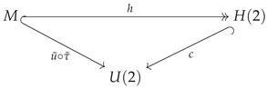
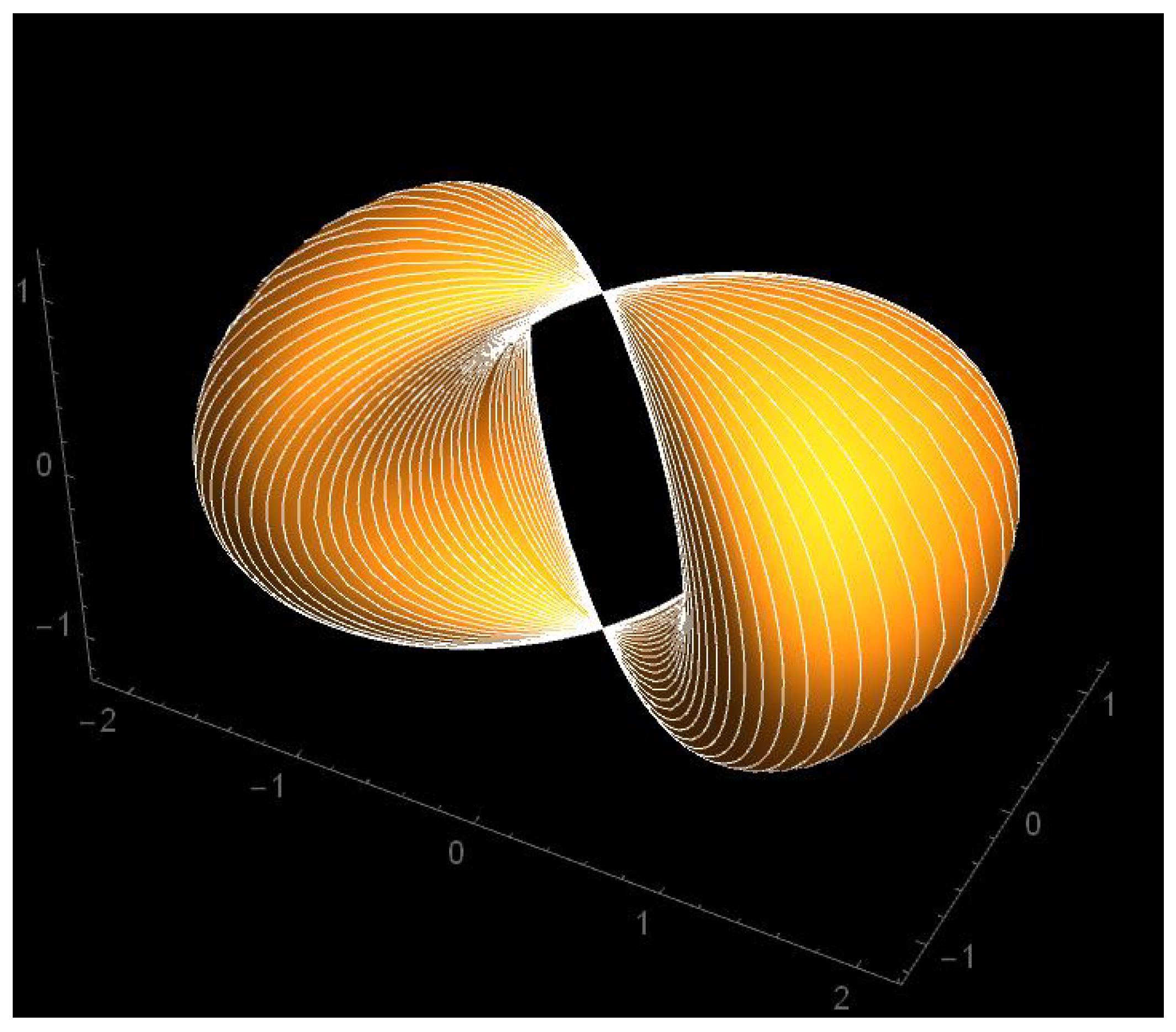
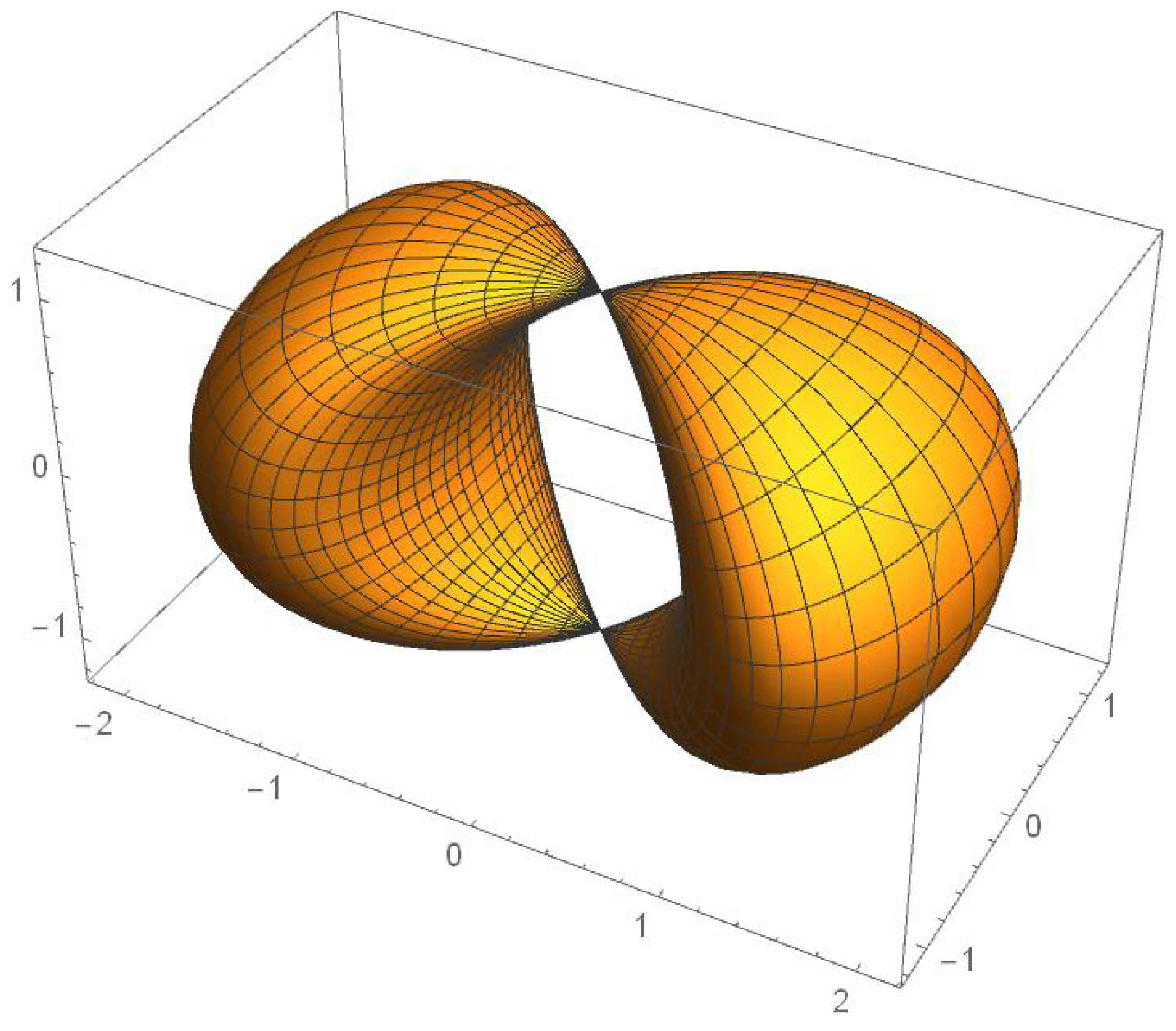
The resulting parametric surface is represented in the following picture:
Essentially, what we have here is a torus, that has been squeezed to a point at two opposite ends.
6.6. Action of the Poincaré Group and Dilations on Conformal Infinity
With the notation as in Sec. , the infinity is characterized by the condition
therefore
If
then
and we get two possibilities
, and
These are the two endpoints in
Figure 1. One can easily check that each of these two endpoints is stable under the action of translations, Lorentz transformations and dilatations. Let us remove these two points from our considerations. Assuming now that
we can chose a unique representative point of the corresponding open subset of
with
We then denote by
u the real parameter
and set
Then every point of the surface is uniquely represented in the form:
where
We obtain an infinite cylinder
If we set
, we get
, , with
Lorentz rotations, translations and dilatations are acting on the conformal infinity leaving this cylinder invariant as a set. We will now calculate the corresponding actions and vector fields corresponding to one-parameter subgroups.
6.6.1. Translations
Eq. (
45) gives us the action of translations subgroup. At the infinity
Skipping the third space coordinate, translation by
is realized by
In order to satisfy Eqs. (
90),(
91) we have to take the quotient by
. Therefore we get the following nonlinear translation transformation:
Taking partial derivatives of
with respect to
at
we get vector fields
– generators of translations:
where
These vector fields are tangent to the infinity surface defined by Eqs. (
90),(
91) and can be expressed in terms of basic vector fields
on this surface. One can easily check that the following formulas hold:
6.6.2. Lorentz Transformations
Let us first consider a pure space rotation:
while
The normalization in this case is unnecessary and differentiating with respect to
at
we obtain the vector field
of pure space rotations:
Next let us consider Lorentz boosts in the direction of the
axis:
while
This time we have to normalize as in Eq. (
108). We get
Differentiating with respect to
at
and using the fact that
, we obtain the vector field
:
Using Eqs. (
99),(100),(
96),(97) we can provide its expression in term of basic vector fields
as follows:
Using the same method we obtain the expression for the generator
D of the dilatations:
A straightforward calculation leads to the Poincaré group (extended by dilatations) commutation relations
6.7. Simple Conformal Infinity
By taking the quotient by ∼ rather than by ≈ we arrive at the same equations (
88,
89), but this time
x and
describe the same point.
Jakob Steiner has faced a similar problem when studying the method of representing the projective plane in
One possible solution was to use quadratic expressions in the coordinates - Cf [
12] and [
13]. Let us first follow a similar method. In order to represent the resulting variety graphically, we will need the following lemma:
Lemma 2.
With the notation as in Section 6.5 introduce the following variables:
Then, assuming that satisfy (90),(91), we have if and only if either or
Proof. The variables
y being quadratic in
it is clear that the ’if’ part holds. Now suppose we have
If
then
therefore from (
91) we have that
and
It follows then from (
90) that
and the same for
Therefore
and
thus
If
then
and
□
6.8. Graphic Representation of Simple Infinity
To obtain a graphic representation we proceed as before and arrive, after renaming of the variables, at the following set of parametric equations
The resulting surface has the shape of a simple elliptic supercyclide
needle (horn) cyclide as in Fig.
Figure 6 - [
14] (Fig. 6, p. 80) [
4 (Fig. 5.7, p. 156), or, in French,
croissant simple [
15]. The surface is, in fact, made of closed null geodesics, all intersecting at the point with homogeneous coordinates
Each od these geodesics is uniquely determined by a point on the 2-sphere
The geodesic is then given by the formula
Figure 2.
Pictorial representation of the simple conformal infinity with one dimension skipped - needle cyclide, made of a one parameter family of null geodesics trapped at infinity.
Figure 2.
Pictorial representation of the simple conformal infinity with one dimension skipped - needle cyclide, made of a one parameter family of null geodesics trapped at infinity.
6.9. Conformal Structure of
Let us begin with a simplified case, with a suppressed
coordinate. As it was described above, in
Section 6.5, we will use the
parametrization. We have the following equations parametrizing
:
Using this parametrization,
we calculate
Since on
we have
, the last two terms cancel, so effectively
Assuming
we easily get
Therefore the metric on our two-dimensional squeezed torus has the form
At the two squeezed points we have and the metric becomes totally degenerate. For other values of u we have a scaled ( by , standard metric on the circles: The metric along the u-lines, connecting the two end-points, is identically zero. Notice that the metric itself is defined up to a scale, since X and , , describe the same point in So, in fact, we have a conformal structure, not a metric.
Let us now return to the full case, including the
coordinate. The calculations become somewhat more complicated, but the end result is similar. Now instead of the coordinate
v we introduce spherical coordinates
and set
Calculating
we get
which is also degenerate:
The part of the metric is the standard metric on the unit sphere in
7. Geometrizing It All - Getting Rid of the Basis
In this section we will make use of the constructions in a paper [
7] by W. Kopczyński and L.S. Woronowicz. They have built a really beautiful and solid foundation. Whenever there is a need, we will adapt their methods to our purposes (for instance in [
7] the authors did not consider the double cover). We will use coordinates only when it is convenient to use them in order to prove some properties. Thus we are allowed to use a basis inside the proof, but not in definitions and in statements about the properties of objects and morphisms. Our reasonings will thus be more abstract, but it will be easier to grasp their geometrical meaning.
In a sense we will repeat all what has been done so far, rephrase it, but now, in definitions and in statements, applying only geometrical invariant concepts.
Let V be a six-dimensional real vector space endowed with a quadratic form of signature Let be the unique scalar product on V such that for all For we will write for
Let
be the null cone of
Q with removed origin:
For
we define the equivalence relation ≈ as
We denote by the equivalence class of X with respect to ≈, and denote by the natural projection.
From now on we define
as
We denote by the group of linear isometries of , i.e. the group of all linear operators for which for all We denote by its subgroup of isometries of determinant one. Notice that for all implies for all Also notice that the determinant of the matrix of a linear transformation does not depend on a choice of a basis.
Proposition 8. The group acts on transitively.
Proof. The proof has been done choosing an orthonormal basis for □
For
and
we will write
We will denote by
the transformation
It is then immediate that the two-element subgroup isomorphic to acts freely on
If p and q are two points in then the property does not depend of the choice of and This fact justifies the following definition:
Definition 2.
For we will write if For any we define as
It is then evident that for
we have
We will call the conformal infinity at p.
Exercise 1. (Why
the conformal infinity at p) Choose an orthonormal basis in V thus identifying V with Choose and Find the explicit form of Identify the points p and on Figure 1.
Exercise 2.
Suppose we want to define the operation of addition on by defining
Can we do this?
Definition 3.
Given any we define
Definition 4.
For let
Exercise 3. Show that the sets are open in (this require some knowledge of topology).
Exercise 4.
where the dot in denotes the fact that we are dealing with a union of disjoint sets.
7.1. Conformal Structure on the Tangent Bundle
The
Section 5.6 can be repeated here without any changes. We did not use coordinates there at all. However we will now discuss in some detail the tangent bundle
of
that is the (disjoint) union of all tangent spaces
As a manifold, is eight-dimensional.
7.1.1. The Tautological Bundle
Every projective manifold comes with a gratis bundle - the tautological bundle. In our case we have the bundle
with one-dimensional fibers
where, for
Thus over each point we have one-dimensional fiber - the subspace spanned by X. Notice that the zero vector of V is in each of these fibers, nevertheless the fibers over different points are disjoint, because, strictly speaking, these "zeros" are ordered pairs and if
Now, since
V is equipped with a scalar product, we also have the orthogonal bundle
where, for
, we have
The fibers of
are five-dimensional. Notice that since
we have
Therefore we can take the quotient bundle whose fibers are the quotient spaces
Using the reasoning in
Section 7.1 about the conformal structure it is clear that the tangent bundle
can be naturally identified with the quotient bundle
Let us choose any such that
Exercise 6. Show that such a q always exists.
Definition 5.
With we define as follows
Remark 7. Notice that is four-dimensional and that, in this definition, Z is assumed to be only in V, not necessarily in . In fact no such Z exists in Proving this is another good exercise.
It is clear from the definition that is a vector space. We can even easily argue that it is four-dimensional - we have two linear conditions on a vector in a six-dimensional space.
We will now construct a vector space isomorphism between and
Proposition 9.
With the notation as above the following map is a vector space isomorphism
where denotes the equivalence class defining the quotient of vector spaces
Proof. Since
Z is in
we certainly have
therefore
Z is in
Let us first see that
is injective. For this it is enough to show that if
then
Now, from the very definition of the quotient of vector spaces it follows that
means that
for some real
If
, then
which contradicts the assumption that
Z is in
Therefore
and so
To prove that
is “onto" it would be enough to bring out the fact that both the domain and the range are vector spaces of the same dimension - four. But it is easy to show it explicitly. To this end, let
be an arbitrary element of the quotient space, with
Now
is not necessarily in
since
is not necessarily zero. Let
Define
Then
and
Therefore Z is in □
Now, since we have already identified the quotient with the tangent space we have a vector space isomorphism between and - different one for different choices of
Let us now recall that, for we have defined as with removed - we remove the infinity cap at If then consists of all those for which Then splits into a disjoint union of and according to whether is positive or negative. Let us concentrate now on the positive case. Then we can always choose Y so that We can therefore construct We will now construct an embedding, which we will denote , of the vector space into the projective null cone manifold such that the image is exactly It is similar to a stereographic map when we embed the plane - the tangent plane at the South Pole p into the sphere, so that the image of this tangent plane is the sphere with removed the North Pole q - the "infinity".
Proposition 10.
Choose a point - an `origin of infinity’. Choose another point and let be its representative in such that The point will be the “origin of the visible `+’ universe". Define
by the following formula:
Then is injective, and its image is exactly
Similarly, if we chose for instance we can set , and define
we obtain an onto diffeomorhism
Before stating the proof we first note that the mapping
is non-linear. It should not be a surprise, since we are wrapping a linear 4-dimensional space
around a compact space
diffeomorphic to
Then we need to show that
is indeed in
that is that
Instead of doing just this, let us contemplate
of a more general form
and find the condition on
so that
is a null vector. Using the facts that
and
we instantly obtain
Therefore is a null vector if and only if
Next, it will be handy to use the following lemma:
Lemma 3.
Let us choose an arbitrary orthonormal basis in thus identifying V with There exists a transformation such that
Proof. Since
acts on
transitively, we can always find a group element that transforms
into
where
After this transformation
will have the form
with
and
To transform further
into
we will use transformations form
that do not affect the point
These are translations, dilatations and 3D rotations. We will use a translation, rotations and dilatations will not be needed. From Eq. (
41) it is clear that translating by
we assure that
takes the form
But then we still have the two conditions:
and
They give us two equations:
and
with a unique solution
□
We will now use this lemma to prove Proposition 8.
Proof. (of Proposition 10) Using Lemma 3 without any lose of generality we may assume that
and
But then our
is the same as
in
Section 6.2, which we already know that it is an embedding. □
7.2. Another Take on Conformal Structure - Null Geodesics
We have identified defined in the Definition 5, with the tangent space Now is a vector subspace of therefore it inherits for V a scalar product. This induces a scalar product on It can be shown that this scalar product is compatible with the conformal structure already defined on - it is a good exercise. With a fixed p but different q these scalar products must thus be proportional (another exercise).
Null geodesics in General Relativity
In this paragraph let
M be a four-dimensional manifold of general relativity. In local coordinates
let
be the metric tensor of signature
Metric tensor induces the Levi-Civita connection
Levi-Civita connection defines covariant derivative
For vector fields we have
A curve
is called a geodesic (or autoparallel) if the tangent vector
parallelly transported along the curve remains tangent to it. This condition entails the equation:
where, for a vector field
denotes the covariant derivative along the path:
One can then always choose a parameter
in such a way that
The geodesic equations become then
Such a parameter is then-called an affine parameter for the geodesic.
Let us see how the geodesic equations (
180) change when we replace
by another metric
in the same conformal class? A straightforward calculation results in
where
If
is an affine parameter for the geodesics of the metric
the equation of geodesics for the new metric become
or, using Eq. (
182):
Assume now that we dealing with a null geodesic, that is that the tangent vector is always a null vector, so that
The last term in (
185) vanishes. Setting
(
185) takes the form of Eq.(
178). Therefore we have the following result
Proposition 11. While in general geodesics for two conformally equivalent metrics are different, null geodesics are the same. They depend only on the conformal structure and not on a particular choice of the representative of this structure.
7.2.1. Coordinate Free Description of Null Geodesics in
is a compact manifold diffeomorphic to
It cannot be covered with one coordinate patch. When we describe null geodesics by geodesic equations, we usee coordinates. Suppose we find a particular solution, a path given in a coordinate system. Then the question arises: and what happens next? How this particular path is going to continue after the coordinates patch ends? In our case one can give an elegant answer to this question by providing a coordinate-free description of a null geodesic, the whole of it, without invoking differential equations. We follow here, [
7], modifying the proof to suit our needs.
Proposition 12.
Get Γ be a two-dimensional isotropic subspace of Then the submanifold
is a null geodesic in Every null geodesic of is obtained this way. If is any point in then the set of all null geodesics through p corresponds to the set of all isotropic planes containing
Proof. In order to show that
is a null geodesic it is enough to show that
can be covered by open neighbourhood, and each of these neighbourhoods is an open segment of a null geodesic. Let
be an arbitrary point of
We will show that
is a null geodesic in a certain neighbourhood of
In order to analyze a neighborhood of
we choose a point at infinity
satisfying
We will now apply the machinery developed in Proposition 10, and use Lemma 3 to introduce an orthonormal basis in
V in which
Here, and in what follows, we will use a shortcut notation, namely we will write
as
understanding that
x is a four-vector. We have now an open neighbourhood
of
that is diffeomorphic to the Minkowski space. Since
is two-dimensional, there exists in
another null vector, linearly independent from
We call it
If we choose
close enough to
the scalar product
will still be positive, and we can scale
so that
From Eq. (
76) we know that
is of the form
where
a is Minkowski space four-vector,
The condition
immediately implies
, thus
a is a null vector in the Minkowski space, therefore
Now every nonzero vector
X in
can be uniquely represented as
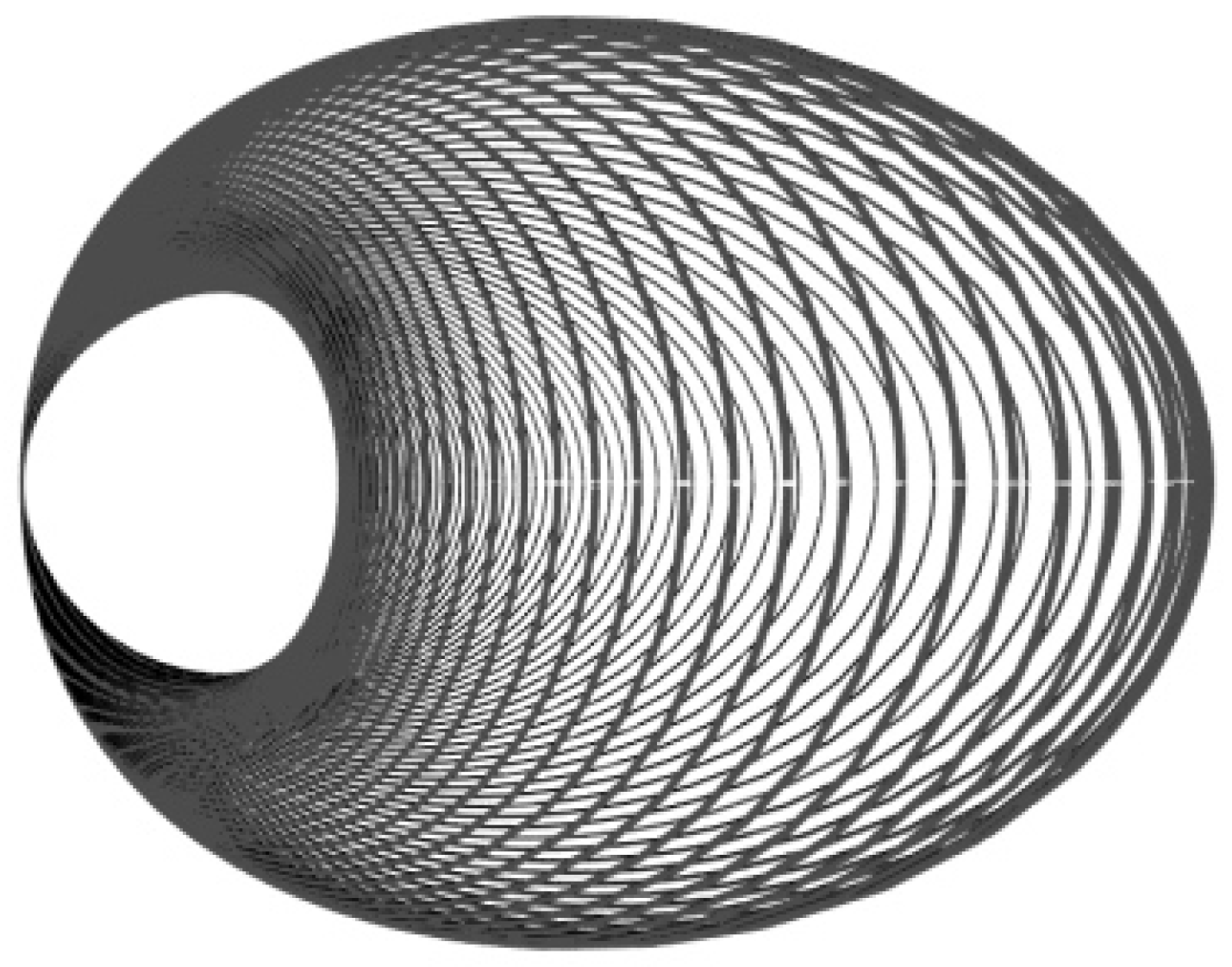
Figure 3.
The pencil (sheaf) of light rays through a space-time point. Temporary illustration.
Figure 3.
The pencil (sheaf) of light rays through a space-time point. Temporary illustration.
Using expressions (
189) and (
192) we get
The scalar product
is positive for
, zero for
and
, and negative otherwise. That means the trajectory is in
for
and crosses the conformal infinity for
and
and is
for other values of
Now that we have a global picture, we concentrate on a neighborhood of the point
Here it is enough to take
which, for
t small enough, is a part of a null geodesic in Minkowski space through the origin, in the direction of the null vector
□
7.3. Light Circling Forever at Infinity and Never Entering Minkowski Space
Given
we have the conformal infinity
at
If
the image by
is contained in
Therefore every null geodesic crossing
p is totally contained in
We will now see how it can be described in coordinates. To this end we will use the parametrization of
as in
Section 6.5. We will use an adapted orthonormal basis in which
. Then any vector orthogonal to
is of the form
where
x is a null vector of the Minkowski space. As we want this vector to be linearly independent of
we must have
In such a case the vectors
and
span the same isotropic plane as
and
Now,
x being a null vector, we can choose it of the form
- it will span, with
the same isotropic plane. Now any vector in this plane is of the form
Comparing the above formula for
with Eqs. (
96), (97) we see that these are exactly the lines of the parameter
u in Eqs. (
101)-(103), which entails the following graphic representation:
Figure 4.
Null geodesics at conformal infinity.
Figure 4.
Null geodesics at conformal infinity.
7.4. Segal’s `Unitime’
Segal’s `chronometric cosmology’ model [
16] differs from the standard cosmological models by the fact that it is based on a priori selected geometry, not Einstein’s theory of General Relativity, even though it uses many of the concepts of General Relativity. The main
physical idea at the foundations of Segal’s cosmology is the
postulate of existence of a distinguished cosmic
time flow - he calls it
unitime. The prefix `uni’ comes probably from the word `unitary’, as it relates to the action of a specific subgroup of the conformal group SO(4,2), a subgroup isomorphic to the one-parameter Abelian group isomorphic to the group
of complex numbers of modulus
A theoretical physicist would probably ask: “Why should it be so? What is the mechanism of such a symmetry braking? Where is the Lagrangian?" But Segal, a mathematician, has an immediate answer to these questions: "Better check if it IS really so as I say, and if it is so, then you will certainly be motivated to find answers to your questions all by yourself."
As we already know
is isomorphic to
In an orthonormal basis, identifying
V with
and
with the manifold of all
such that
The action of
corresponds to the Euclidean rotation of the
coordinates, other variables being fixed:
Notice that now we pay attention to the physical dimensions and have replaced the parameter s with and have replaced 1 on the right-hand-side of the above equations by a dimensional constant R - the `radius of the universe’.
Remark 8. In such an approach the `flow of time’ has an objective reality. Which agrees with our observations of reality - if flow of time would be entirely subjective, it would be impossible to explain why most of the people agree on the duration of time sequences of events and respect their friends’ birthday dates.
Remark 9. Speaking about `physics’: Segal allows s to be going from minus infinity to infinity, nor just from 0 to In other words we replace by its universal cover, that is by Cosmology becomes cyclic. We have an infinite number of cycles. There is still a question about what is the elementary cycle? Should we identify X with , or not? Is the Minkowski space simple or doubled? Usually it is assumed that it is a simple one, therefore already the interval is assumed to be a cycle. I see no valid reason for such a postulate.
Let us see how Segal’s `unitime’ relates to the coordinate time of the Minkowski space. To this end let us analyze the `unitime line’ through the origin of the Minkowski space in adapted coordinates. We represent Minkowski space event with coordinates
x by its image
as in Eq. (
76). The origin is then represented by
therefore, using Eqs. (
199), the unitime line becomes
In order to find
we divide
by
to obtain
The space origin
remains constant. We see that the unitime line is the same as the time line of the Minkowski space, but
the rate of time is different. Developing into the Taylor series we get
The difference between the two times becomes significant only for big enough in the R-scale.
7.5. Guessing the Metric
In this section, to simplify the notation, let us call the
coordinate simply
t (assuming units in which
). Inverting Eq. (
205) we have
Let us now try to find a metric in the conformal class of the flat Minkowski metric for which
s would be the proper time on the unitime line. We look for a metric of the form
Along the time line
therefore, for the proper time parameter
s we get
Using Eq. (
208) we obtain
8. Compactified Minkowski Space as a Boundary of Five-Dimensional Domains
The null cone
of
V separates two domains
characterized as follows:
Let us consider their projections
(resp.
) obtained by taking the quotient by the equivalence relation
For every point of
(resp.
) there is a unique point
X in
(resp.
) for which
(resp.
Therefore,
can be, respectively, identified with a five-dimensional hyperboloid
defined by
Now is a topological boundary of and of , a four-dimensional boundary that separates these two five-dimensional domains.
Let us look now at the topology of the two five–dimensional domains
For the domain
we have the defining equation
It is then clear that
and
can be arbitrary real numbers, and that introducing
we have
Therefore,
has the topology of
Proceeding the same way with
we have
that is
Therefore has the topology of
8.1. A Coordinate Description of
In
we choose an open set defined by the condition
On this set we introduce five coordinates
defined by
On the other hand, given a point in
with coordinates
we can embed it in
as follows:
Reader is encouraged to verify by a straightforward calculation that with the above definition
and that applying formula (
220) to
we indeed recover
We can now calculate a new metric. In general, when we are dealing with an embedded manifold parameterized by coordinates
its metric
is induced by a metric
on a manifold into which our manifold is embedded, and it is given by the expression
In our case,
and it is easy to calculate
using formula (
221). The result of a straightforward calculation is:
Exactly the same method applies to the region
We get a five–dimensional pseudo–Riemannian, conformally flat manifold of constant curvature and signature
We have covered by coordinates two regions corresponding to different signs of the fifth coordinate. Physicists, when discussing representations of the conformal group with applications to elementary particle physics, often restrict their attention to these regions - Cf. for instance [
22?,
23]. Yet, evidently the group
acts on this part with singularities. Like in the case of Minkowski space, in order to avoid singularities one has to add “conformal infinity”. In our case this is a region where
This conformal infinity of the five–dimensional domain has a simpler structure than the one for the Minkowski space. In fact, setting
in (
216), we get
with no scaling freedom. Therefore, the conformal infinity of our five–dimensional domain
is the Cartesian product of
(
) and the standard two-sheeted hyperboloid of the Minkowski space.
8.2. Christoffel Symbols and Geodesics
Given metric (
223) it is easy (in our coordinate patch) to calculate the Christoffel symbols
and geodesic equations - see e.g. [
24] (Mathematica Programs: Christoffel Symbols and Geodesic Equations). The metric is conformally flat and the only non–vanishing Christoffel symbols are:
The corresponding geodesic equations, when parameterized by an affine parameter
s, are:
where
and
is the flat Minkowski metric
It is interesting to notice that, for
Minkowski’s space null lines
where
is a fixed null vector, are geodesics of the five–dimensional space.
When
is non–constant, it is convenient to choose
as a (non–affine) parameter. The geodesic equations will read in such a case (adapted from [
19] (Appendix B, (B7))) as
which, in our case, reduces to:
Here, we denote by a prime the derivative with respect to
and denote
The direction of the vector
is kept constant along the geodesics. Thus, we need to consider three cases:
and
If
we can use a Lorentz rotation (in the variables
) to set the direction of
along the vector
The differential equations reduce in this case to the following ones:
which, taking into account the constraint
solve to
with
and
constant.
When
we can use a Lorentz rotation to rotate the geodesic into the
plane. The relevant differential equation:
solves to
- a hyperbola.
When
we can Lorentz rotate the geodesic into the
plane, and the differential equation
solves to
- a semi–circle.
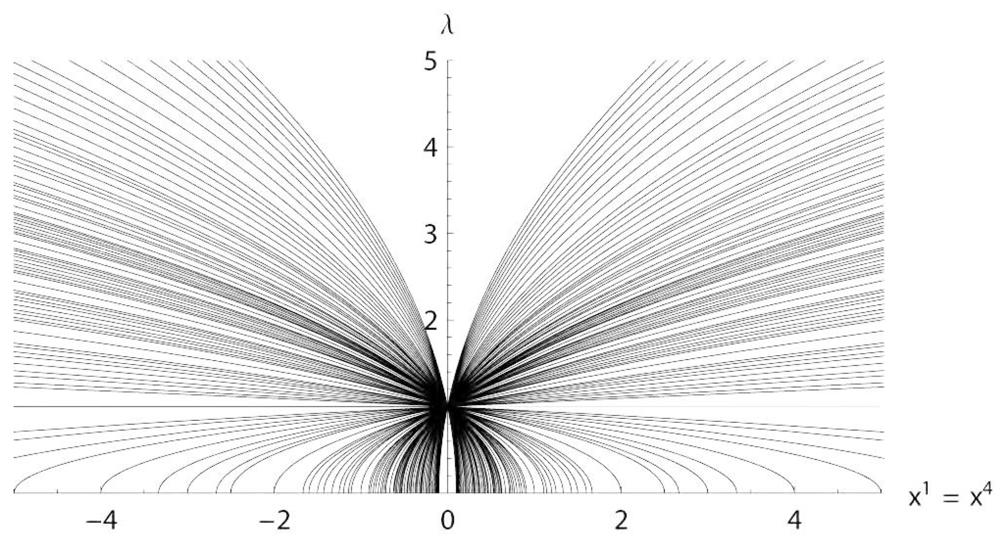
Figure 5.
A family of geodesics in the plane through the point
Figure 5.
A family of geodesics in the plane through the point
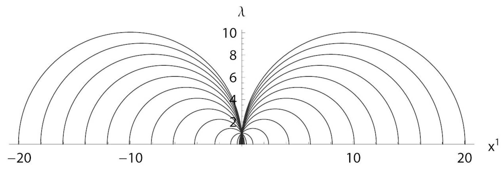
Figure 6.
A family of geodesics in the plane through the point .
Figure 6.
A family of geodesics in the plane through the point .
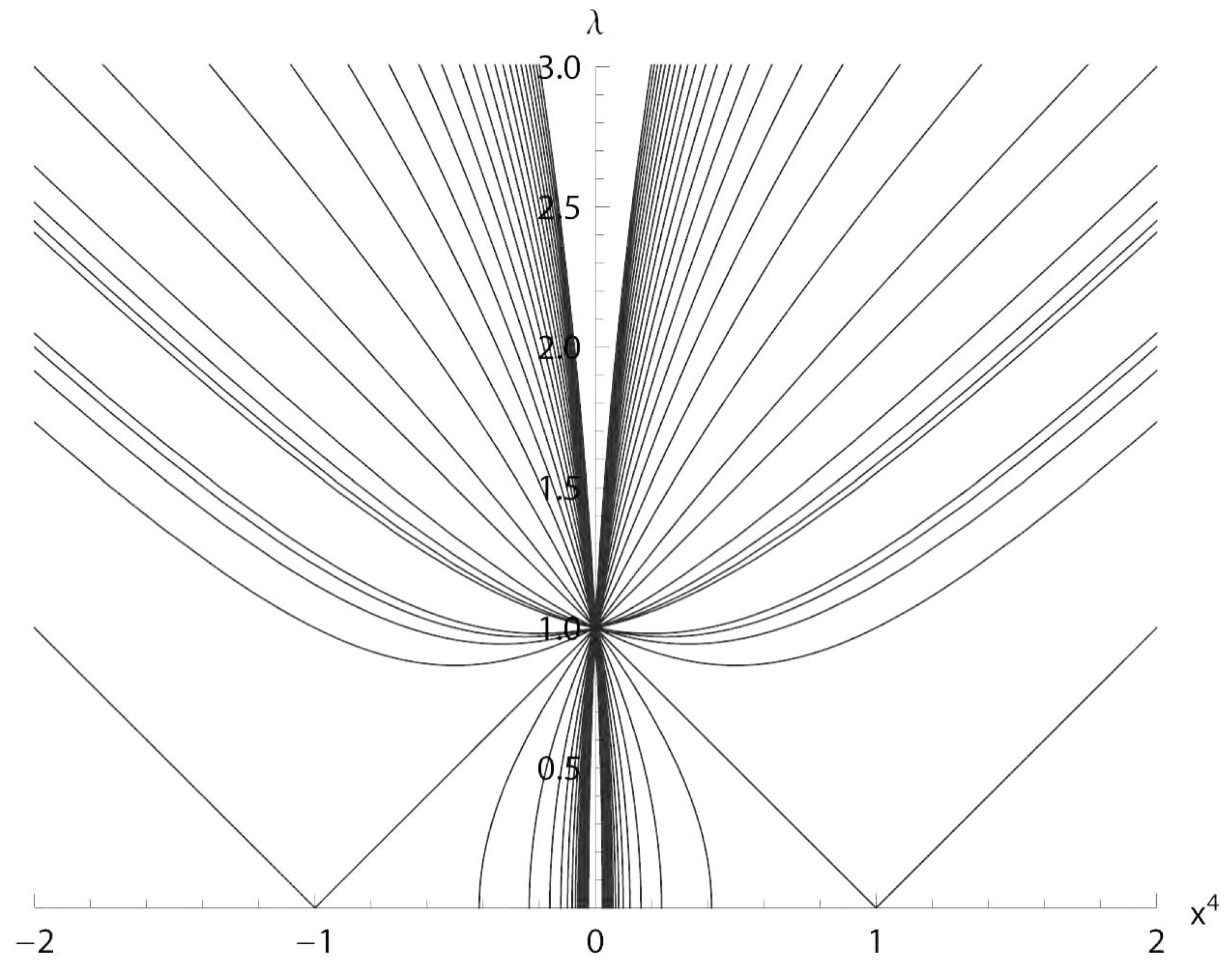
Figure 7.
A family of geodesics in the plane through the point .
Figure 7.
A family of geodesics in the plane through the point .
8.3. as the Space of Hyperboloids
The five–dimensional homogeneous space
can be interpreted as a space of (unoriented) hyperboloids in the Minkowski space along the lines of a generalized Möbius geometry (Cf. e.g., [
4] (Ch. 1.2)). Let
Y be in
with
and
Consider a set of all
for which
Normalizing
Y so that
we can write it in the form
A simple calculation shows that the condition
translates then to
For
this is a double-sheeted hyperboloid with apex at
Each geodesic line in
can thus be interpreted as a particular one–parameter family of hyperboloids in the Minkowski space.
8.4. The Case of
The same method as above applies in this case except that there is a change of signs in front of
in (
221). The resulting metric is then
with signature
As in the case of
, the conformal infinity is the Cartesian product of
and, this time, the one-sheeted hyperboloid
The Minkowski space can be embedded in our five–dimensional manifold simply by putting It follows that the direction of the vector is constant along the geodesics.
Remark 10. Following Wolf [25] we have considered in detail only the case of the equivalence relation In projective geometry one is using the weaker relation The standard projection can be discussed along the same lines as above. In that case the regions and are identified, so we can restrict our attention to 2 On the other hand, when discussing the topology - we have to additionally take the quotient by
9. Conclusions
In this work the conformal compactification of Minkowski space has been revisited in an explicit and pedagogical manner, starting from the projective null cone in and its identification with the unitary group . The role of the double cover has been clarified, with particular emphasis on the effectiveness of the action and on the detailed geometry of conformal infinity, described in terms of horn and needle Dupin cyclides. By combining concrete coordinate constructions, explicit matrix formulas for the conformal group and its subgroups, and a coordinate-free reformulation in the spirit of Kopczyński and Woronowicz, the paper aims to provide a transparent geometric picture that can serve both as a reference and as a pedagogical introduction to conformal compactification in mathematical relativity and conformal field theory.
Acknowledgments
Thanks are due to R. Coquereaux for his interest and for a stimulating discussion on related subjects at the early stage of this work. I wish to thank my wife, Laura, for her constant support. This work was supported by Quantum Future Group Inc.
Conflicts of Interest
Author declare no conflict of interest.
References
- Penrose, R.; Rindler, W. Spinors and space-time; Cambridge University Press, 1986; ISBN 0521347866. [Google Scholar]
- Uhlmann, A. The Closure of Minkowski Space. Acta Physica Polonica 1963, Vol. XXIV, Fasc. 2(8), 295–296. [Google Scholar]
- Barbot, T.; Charette, V.; Drumm, T.; M. Goldmann, W.N.; Melnick, K. A primer on the (2+1) Einstein universe. [CrossRef]
- Cecil, Thomas E. Lie Sphere Geometry, 2nd ed.; Springer, 2008. [Google Scholar]
- Morava, J. At the boundary of Minkowski space. arXiv [math-ph]. 2021, arXiv:2111.08053v3. [Google Scholar] [PubMed]
- Lester, J.A. Conformal Minkowski Space-time. Il Nuovo Cimento 1982, 72 B(N. 2), 261–272. [Google Scholar] [CrossRef]
- Kopczyński, W.; Woronowicz, L.S. A Geometrical Approach to the Twistor Formalism. Reports on Mathematical Physics 1971, 2, 35–51. [Google Scholar] [CrossRef]
- Lester, J.A. Orthochronous Subgroups of O(p,q). Linear and Multilinear Algebra 1993, Vol. 36, 111–113. [Google Scholar] [CrossRef]
- Shirokov, D.S. Lectures on Clifford Algebras and Spinors. Available online: https://www.researchgate.net/publication/267112376_Lectures_on_Clifford_algebras_and_spinors.
- Mneimné, R.; Testard, F. Groupes de Lie classiques; Hermann, 2009; ISBN 9782705660406. [Google Scholar]
- Werth, J.-E. Conformal Group Actions and Segal’s Cosmology. Reports on mathematical physics 1986, 23, 257–268. [Google Scholar] [CrossRef]
- Artmann, Benno. PICTURES of the PROJECTIVE PLANE, in Günter Törner, and Bharath Sriraman. Beliefs and Mathematics: Festschrift in Honor of Günter Törner’s 60th Birthday; Charlotte, NC, Information Age, 2008; Available online: http://www.math.umt.edu/tmme/Monograph3/Artmann_Monograph3_pp.3_16.pdf.
- Hilbert, D. S Cohn-Vossen Geometry and the Imagination; Ams Chelsea: Providence, Ri., 1999; ISBN 9780821819982. [Google Scholar]
- Schrott, M.; Odehnal, B. Ortho-Circles of Dupin Cyclides. Journal of Geometry and Graphics 2006, 1, 73–98. Available online: http://www.heldermann-verlag.de/jgg/jgg10/j10h1schr.pdf.
- Feréol, R. Cyclide de Dupin. Available online: https://www.mathcurve.com/surfaces/cycliddedupin/cyclidededupin.shtml (accessed on 25 June 2024).
- Segal, I.E. Mathematical Cosmology and Extragalactic Astronomy; Academic Press, 1976; ISBN 9780080873848. [Google Scholar]
- Berestovskiĭ, V N. To the Segal Chronometric Theory. Siberian Advances in Mathematics 2023, 33(no. 3), 165–180. 165–180. Available online: https://arxiv.org/pdf/2404.06866. [CrossRef]
- Ingraham, R.L. Conformal Relativity. Proceedings of the National Academy of Sciences of the United States of America 1952, 38, 921–925. [Google Scholar] [CrossRef] [PubMed]
- Müller, T.; Weiskopf, D. Detailed Study of Null and Timelike Geodesics in the Alcubierre Warp Spacetime. General Relativity and Gravitation [gr-qc]. 2011, arXiv:1107.565044, 509–533. [Google Scholar] [CrossRef]
- Huggett, S.A.; Tod, K.P. An Introduction to Twistor Theory; Cambridge University Press, 1994; ISBN 9780521456890. [Google Scholar]
- Daigneault, A. Irving Segal’s Axiomatization of Spacetime and Its Cosmological Consequences. arXiv (Cornell University) 2005. [Google Scholar]
- Ingraham, R.L. Conformal Relativity. Proceedings of the National Academy of Sciences of the United States of America 1952, 38, 921–925. [Google Scholar] [CrossRef] [PubMed]
- Ingraham, R.L. Particle Masses and the Fifth Dimension. Annales de la fondation Louis de Broglie/Annales de la Fondation Louis de Broglie 2000, 29, 989–1004. [Google Scholar]
- Hartle, J.B. Cambridge University Press Gravity: An Introduction to Einstein’s General Relativity; Cambridge Cambridge University Press; ISBN 9781316517543, 2021; Available online: http://web.physics.ucsb.edu/~gravitybook/math/.
- Wolf, J.A. Spaces of Constant Curvature; American Mathematical Society, 2023; ISBN 9781470473655. [Google Scholar]
- Juergen, Elstrodt; Grunewald, F. Jens Mennicke Groups Acting on Hyperbolic Space; Springer Science & Business Media, 2013; ISBN 9783662036266. [Google Scholar]
- Paul, T.; Penrose, R. Penrose’s Weyl Curvature Hypothesis and Conformally-Cyclic Cosmology. Journal of physics 20. Penrose, R. On the Gravitization of Quantum Mechanics 2: Conformal Cyclic Cosmology. Foundations of Physics 2013, 44, 873–890. [Google Scholar]
| 1 |
Ref. [ 11] (Proposition 8) ascertains the existence of the action of on . Here we have its explicit realization |
| 2 |
That is why a similar coordinatization is often referred to as the “half–space model” in literature on hyperbolic geometry - see e.g. [ 26]. |
|
Disclaimer/Publisher’s Note: The statements, opinions and data contained in all publications are solely those of the individual author(s) and contributor(s) and not of MDPI and/or the editor(s). MDPI and/or the editor(s) disclaim responsibility for any injury to people or property resulting from any ideas, methods, instructions or products referred to in the content. |
© 2026 by the authors. Licensee MDPI, Basel, Switzerland. This article is an open access article distributed under the terms and conditions of the Creative Commons Attribution (CC BY) license (http://creativecommons.org/licenses/by/4.0/).