
Submitted:
31 December 2025
Posted:
01 January 2026
You are already at the latest version
Abstract
This study revisits the Efficient Markets Hypothesis by employing a GRU-D neural network to predict stock return distributions across global equity markets, accounting for missing and irregular data. It examines whether stock returns exhibit statistically significant departures from purely random behavior. By combining price, technical and fundamental inputs, it tests both weak and semi-strong market efficiency.
We implement the GRU-D model on a global dataset of stock returns, where daily returns are classified into quartiles. Model performance is assessed using Micro-Average Area Under the Curve (AUC) and Relative Classifier Information (RCI). Robustness checks include sub-sample tests across countries and sectors, an examination of the Covid-19 sub-period, and a price-memory persistence analysis.
The results reveal that the GRU-D model achieves a ranking accuracy of approximately 75% when classifying returns, with a statistical significance at the 99.99% confidence level, and exhibits modest but robust deviations from strict market efficiency. These deviations persist for up to 200 trading days. Notably, the findings indicate that the GRU-D model is more robust during the Covid-19 period.
These findings are consistent with the Adaptive Markets Hypothesis and underscore the relevance of machine-learning frameworks, particularly those designed for imperfect data environments, for identifying time-varying departures from strict market efficiency in global equity markets.
Keywords:
efficient market hypothesis
; returns prediction
; machine learning
; GRU-D
1. Introduction
The Efficient Market Hypothesis (EMH) is one of the most influential and widely debated concepts in neoclassical finance. It asserts that asset prices fully and continuously reflect all available information (Fama, 1970). Market efficiency theory examines whether markets can form prices that accurately capture the fundamental value of financial assets. Rational investors react to new information, updating expectations and adjusting asset prices. When observed returns deviate from CAPM predictions, anomalies arise, challenging the EMH.
Empirical studies have shown that CAPM alone cannot explain certain asset-pricing anomalies. To address these limitations, multi-factor models were introduced, incorporating additional factors that capture specific risk exposures and market anomalies. The Fama-French three-factor model (Fama & French, 1993) adds size and value factors to market risk, while the five-factor model (Fama & French, 2015) further includes a firm’s profitability and momentum.
Behavioral finance complements this perspective by questioning investor rationality and emphasizing the influence of cognitive biases, such as overconfidence, herding, loss aversion and anchoring. Studies by Daniel et al. (1998), Barberis et al. (2001) and Baker and Wurgler (2006) integrate behavioral proxies into traditional asset pricing models, demonstrating that investors’ behavior and psychology significantly shape asset prices. Despite these advances, no single comprehensive model exists due to the complex interaction of behavioral and market factors. Recent studies, such as Li and Wu (2023), have extended the three-factor model by incorporating investor sentiment from online stock bar text data, highlighting the growing role of behavioral indicators in asset pricing models.
Traditional econometric methods, such as linear regression and time-series models, remain valuable for their interpretability and analytical simplicity. However, their reliance on linearity and low-dimensional data limits their effectiveness when facing the complexity, nonlinearity, and scale of modern economic and financial systems. As data becomes larger and more intricate, researchers increasingly turn to hybrid approaches that integrate traditional models with machine learning techniques to enhance predictive accuracy, uncover hidden patterns, and address complex problems (Sonkavde et al., 2023; Doe, 2024).
In this context, recurrent neural network architectures, and specifically the Gated Recurrent Unit with Decay (GRU-D) model, offer significant methodological advantages. GRU model offers advantages such as computational efficiency, faster training, and the ability to capture long-term dependencies in sequential data, making it ideal for tasks like time series forecasting and stock price prediction. More precisely, the GRU-D model is designed to handle missing or irregularly spaced data by incorporating a decay mechanism that adjusts the influence of past observations based on the time elapsed, improving prediction accuracy in complex time series scenarios (Che et al., 2018; Sonkavde et al., 2023).
The objective of this study is to employ the GRU-D model to test the weak and semi-strong forms of market efficiency in financial time series, where irregular and incomplete observations are common. In line with prior studies on market efficiency that distinguish between information sets (Fama, 1970), the model is specified to incorporate variables associated with weak-form efficiency (past prices and technical indicators) and semi-strong-form efficiency (financial ratios and fundamental indicators). The strong form is excluded, as it requires access to insider information that is unavailable. The study examines whether stock returns exhibit a predictive structure that significantly exceeds the random baseline. Demonstrating that the GRU-D consistently delivers statistically significant improvements over chance constitutes direct evidence against strict market efficiency (Pagliaro et al., 2025). To ensure external validity, predictive performance is further evaluated across countries, sectors and time periods, thereby capturing heterogeneity in economic conditions and institutional settings.
This study has several contributions. From a methodological perspective, and to the best of our knowledge, it is the first to apply the GRU-D framework to test market efficiency. Its capacity to handle missing data and capture complex temporal patterns enables a more nuanced understanding of market behavior, overcoming the limitations of traditional tests that rely on fully specified asset pricing models (Fama, 1991). For practitioners, this study presents a framework that detects persistent and significant inefficiencies with minimal preprocessing.
Furthermore, by identifying markets, sectors, or periods with greater deviations from strict market efficiency, investors can better calibrate their risk exposure and seek arbitrage opportunities. Our research also serves as a benchmark for future comparisons with both classical models and alternative neural architectures. For regulators, our results offer a diagnostic tool to monitor how efficiently information is reflected in asset prices. Persistent market inefficiencies highlight areas where market transparency and disclosure practices could be strengthened.
2. Literature Review: Market Efficiency and Machine Learning Models
Today, most market transactions are executed by algorithms, fundamentally altering market microstructure. This shift has accelerated the adoption of machine learning (ML) in finance, where systems learn patterns from historical data and optimize decisions without manual programming. ML is a subset of artificial intelligence (AI) that encompasses techniques enabling computers to emulate human reasoning and solve complex tasks with minimal human input (Russell & Norvig, 2010). While early AI focused on explicit rules and formal logic, ML allows systems to learn from data, overcoming limitations of traditional approaches.
The rapid expansion of financial data has outpaced human analytical capacity, prompting increased reliance on AI and deep learning methods. These approaches can process diverse unstructured data, including text, images and videos, allowing for the identification of novel determinants of asset prices. Recent evidence suggests that such models often surpass traditional econometric approaches in predictive accuracy (Sirignano & Cont, 2019).
Clustering techniques, such as k-means and hierarchical clustering, have been used to group assets based on historical price patterns, revealing insights beyond conventional market classifications. For instance, Li et al. (2023) combined k-means clustering with Long Short-Term Memory (LSTM) models to group U.S. stocks, achieving strong forecasting performance.
A systematic review by Kumbure et al. (2022) of 138 stock market prediction studies (2000–2019) found that Artificial Neural Networks (ANNs), Support Vector Machines (SVMs) and fuzzy logic were most applied.
Several studies illustrate the practical applications of ML in financial forecasting. Dimitriadou et al. (2018) predicted WTI oil prices using SVM with a nonlinear Radial Basis Function kernel. Diamond and Perkins (2022) challenged the semi-strong EMH across asset classes using ML techniques, including Logistic Regression, Random Forest, Gradient Boosting, SVM and ANN, demonstrating that intermarket information improves predictive accuracy. Machine learning has also proven effective in credit risk assessment by exploiting alternative data to reduce information asymmetry and improve prediction accuracy (Mhlanga; 2021).
In recent years, LSTM and GRU architectures have gained prominence for their robustness and superior predictive performance in financial time-series. Patel et al. (2020) combined LSTM and GRU to forecast cryptocurrency prices, while Lee and Yoo (2020) compared RNN, LSTM and GRU models for predicting S&P 500 stock returns, concluding that LSTM outperformed the others. Similar findings were reported by Yao and Yan (2024) and Dželihodžić et al. (2024), who highlighted LSTM and GRU’s superiority over CNN and conventional RNN models. This conclusion is supported by a recent systematic review, which shows that GRU and LSTM models excel in financial time-series prediction. GRU is faster and less prone to overfitting, while LSTM captures long-term dependencies (Sonkavde et al., 2023).
Region-specific applications include Li et al. (2020) for Hong Kong, Budiharto (2021) for Indonesia, Yadav et al. (2020) for India, Samarawickrama and Fernando (2017) for Sri Lanka and Nti et al. (2020) for Ghana. Hossain and Kaur (2024) demonstrated the complementary strengths of XGBoost and LSTM for U.S. ETFs. Kadam et al. (2024) further explored the nuances of LSTMs and GRUs, guiding the choice of financial forecasting models. Finally, Shahi et al. (2020) showed that incorporating financial news sentiment into LSTM and GRU models significantly improves stock price prediction. The LSTM-News and GRU-News models achieved superior accuracy compared to models relying solely on market data.
3. Research Design
3.1. Data and Sample
Given the unique characteristics of each asset type and the availability of data, we have chosen to focus on the stock market. One of the most reputable financial sources is Yahoo!Finance. We used the yfinance library, which enables downloading and manipulating data using Python. To exploit the application programming interface, we have prepared a script that allows us to browse and download a sample from the data available in a list of 106,328 stock tickers provided by “investexcel”. This script browses the list of these tickers to download the data available from yfinance, which provides coverage for 9,686 tickers.
Our collected data sample includes 83 predictor variables. The data excluded from our selection includes unstructured data (primarily textual) and data for which we have no publication date. The categories of variables collected are summarized below:
- -
- Asset prices time series data OHLC - (Open, Low, High, Close and Volume) with daily frequency.
- -
- Financial data with a total of 50 data points [1] as well as their publication dates, which generally fall in the third month of each year (March). These data comprise 28 balance sheet variables and 22 income statement variables.
- -
- Fundamental data with a total of 27 data points (such as PER, ROE, ROA), including their publication date.
The final database includes 9,686 assets distributed across 32 countries and 47 economic sectors [2], spanning 10 years and 40 days from July 27, 2011, to September 6, 2021. Each asset has an average observation window of 5,800 days. The United States tops the list, accounting for approximately 50% of the database.
3.2. Data Preprocessing
To predict future asset returns, a data preprocessing phase is required. This phase involves transforming independent variables, extracting predictor features and defining the dependent variable. Variable transformation includes computing logarithmic returns and calculating financial ratios from accounting data. New predictor variables are generated from seasonal patterns and chartist indicators. The dependent variable is defined by discretizing returns into categorical classes.
3.3. Variables Construction
3.3.1. Dependent Variables
We calculated the daily logarithmic returns of the adjusted closing price and then classified them into discrete return quartiles (Hu et al., 2021). The use of four categories reflects a trade-off between granularity and simplicity of implementation in the predictive framework. The four classes are defined as follows:
Class 1: Includes returns falling below the first quartile. These represent the lowest returns in our dataset, indicating a decrease in asset prices.
Class 2: Includes returns that are equal to or greater than the first quartile but less than the median of the logarithmic returns. These returns are in the lower-middle range.
Class 3: Includes returns that are above the median but less than the third quartile, placing them in the upper-middle range of returns.
Class 4: Includes returns that are equal to or exceed the third quartile, denoting the highest returns.
3.3.2. Independent Variables
The following variables proxy for weak-form market efficiency [3]:
- -
- Raw data on asset prices and logarithmic returns: The raw data includes asset prices (open, close, high, low and trading volume) and adjusted closing prices. These prices are transformed into logarithmic returns.
- -
- Seasonal data: Two variables are included in this category. The first variable is the day of the week, which takes values 1-5 (Monday-Friday). The second variable denotes the calendar week of the year, taking values from 1 to 52. These variables try to capture well-documented market anomalies such as the weekend effect (Penman, 1987) and the January effect (Ariel, 1987).
- -
- Chartist indicators: They were selected using the approaches proposed by Prachyachuwong and Vateekul (2021) and Sirucek and Šíma (2016). The set of indicators includes the Relative Strength Index, Moving Average Convergence Divergence and Chande Momentum Oscillator, among others [4].
Regarding the semi-strong form of efficiency, the selected variables related to fundamental data encompass financial ratios, financial statement information (Alexakis et al., 2010) and governance or competition-related measures (Bodie et al., 2009) [3]. The variables are organized into three categories and scaled to allow for comparability across firms: Balance sheet items are scaled by total assets and income statement items are normalized by total revenue. Additional fundamental data included sector classification, governance indicators and measures of market competition.
3.4. Experimental Design
This section outlines the empirical design underlying the framework used to test market efficiency. It first details the construction of the database and the generation of training and test samples within a rolling-window framework that preserves temporal ordering and closely mimics real-time forecasting conditions. Training samples are used to estimate model parameters by minimizing a cross-entropy loss function. The loss function measures the discrepancy between the model’s predictions and the actual target values. The testing sample provides out-of-sample predictions. The learning phase further refines this optimization process by adjusting model weights to minimize the loss function. The GRU-D model is implemented in PyTorch [5], with parameter calibration, model estimation and predictive validation.
3.4.1. Training and Testing Design
A large dataset enables the model to detect reliable relationships among variables and support robust estimation. The training set consists of 6,000 observations, representing 12% of the dataset. This subset was constructed to reflect the heterogeneity of the sample, which spans multiple sectors and countries. The geographical distribution is led by U.S. firms, with significant representation from Germany, France and Canada. The relatively small training set reflects hardware constraints, particularly memory limitations during model estimation.
After selecting assets with sufficient data coverage, we constructed the model inputs using a rolling-window approach. This procedure, commonly adopted in financial forecasting, trains the model on fixed-length sequences of past observations to predict the subsequent value. The window then advances by one period, generating a new input–output pair. Repeating this process yields a large set of training instances, allowing the model to learn temporal patterns while closely mimicking real-time forecasting conditions. To account for varying degrees of temporal dependence, we considered alternative window lengths, as described in the learning phase below
3.4.2. The GRU-D Model Implementation
The GRU-D model was implemented using Han-JD’s [6] open-source Python code, based on the PyTorch library, which provides a flexible environment for sequential data modeling. In its original binary setting, the output layer consisted of a single unit, trained with a binary cross-entropy loss that compared the predicted probability to the actual outcome. In this study, the output layer- that is, the final step of the model where predictions are generated- was redefined with four units corresponding to our four classes of return. The multi-class cross-entropy loss function evaluates how well the predicted probability distribution matches the true class. The Softmax function converts raw model returns into probabilities, ensuring that all class probabilities sum to one (Razali et al., 2025; Terven et al., 2025).
3.4.3. Learning Phase
A distinctive feature of GRU-D is its ability to incorporate missing or irregular observations directly into the learning process. To achieve this, the model uses vectors indicating which values are missing and how much time has elapsed since the last observation. A global mean vector, computed from the average of each variable in the training data, is used to impute missing values. Inputs are thus represented as observed values, missingness indicators and time gaps, enabling the GRU-D to learn from both financial variables and the structure of missing data via temporal decay [7].
Building on the dataset construction and rolling-window design described previously, the GRU-D model’s learning phase was implemented in two stages. In the first stage, we conducted a hyperparameter search to identify the most suitable specification for our prediction task. The configurations varied along several key dimensions: the observation window length, the network complexity (number of hidden layers), the learning rate (speed of parameter updates) and the training duration (number of epochs). This trade-off between horizon and complexity is consistent with prior applications of recurrent architectures in financial forecasting (Fischer and Krauss, 2018; Hu et al., 2021). This exploration phase will allow us to evaluate alternative setups and determine the configuration that yields the most stable and efficient learning outcomes, as measured by the loss function. In the second stage, the training process was extended using the optimal hyperparameters to further enhance the model’s predictive performance. Five model specifications were evaluated, combining alternative observation window lengths (200, 400 and 600 days) with hidden-layer sizes of either 150 or 300 units.
To manage computational cost while ensuring stability, training was organized in two phases. The first phase involved 20 epochs for model selection, while the second extended the final configuration to 40 epochs. Optimization was performed using the Adam algorithm [8] with an initial learning rate of 0.01, halved every 10 epochs to ensure convergence. Each configuration was trained five times to account for initialization randomness, with an average training time of 4 hours and a maximum of 8 hours for the most complex models. This regimen ensured robust, reproducible performance across runs, in line with recommendations from prior studies (Sirignano and Cont, 2019).
Figure 1 illustrates this two-stage training process. Among the tested configurations, the green curve corresponds to the specification with a 400-day observation window and 300 hidden layers. This configuration achieved the lowest training loss, indicating it minimized the gap between predicted and actual values during training.
To mitigate concerns about overfitting, we validated the model on a substantially larger, more diverse testing set comprising 45,894 observations (88.4% of the dataset). This design allows the model’s generalization ability to be rigorously evaluated across different sectors and countries. As shown in Figure 2, training loss (red curve) declined steadily from 1.22 to 1.15, while validation (green) and testing losses (blue) stabilized around 1.18 and 1.17 after epoch 10. The close alignment of these loss curves indicates that the model learned real patterns that also worked on unseen data.
4. Empirical Results and Discussion
4.1. Predictive Power of the GRU-D Model
The AUC represents the area under the ROC (Receiver Operating Characteristic) curve. The ROC curve is a graphical representation of a classifier’s diagnostic performance, plotting the true positive rate (the proportion of correctly identified positive cases) against the false positive rate (the proportion of negative cases incorrectly classified as positive) across varying classification thresholds. By summarizing the ROC curve into a single value, the AUC captures the model’s overall discriminatory power across all possible thresholds. AUC values range from 0 to 1, where a value greater than 0.5 corresponds to a discriminative ability superior to mere chance (Che et al., 2018).
We computed the Micro-Average AUC, which aggregates performance across all observations and thus provides a more representative measure of the model’s overall discriminative ability under class imbalance (Fawcett, 2006; Saito & Rehmsmeier, 2015). AUC values for each of the four return categories illustrate the model’s ability to accurately classify different levels of returns. The results are reported in Table 1. The Micro-Average AUC is 0.75, with a tight 99.99% confidence interval of [0.7454, 0.7471], indicating that the model correctly ranks positive versus negative outcomes 75% of the time. This value is considered acceptable (Luo et al., 2025), suggesting that the GRU-D captures meaningful financial signals.
The predictive performance is not evenly distributed across classes. It is concentrated on the extremes of the return distribution, with the model more effective at identifying the lowest returns (Class 1, AUC = 0.684). This asymmetry suggests that violations of EMH signals are most pronounced in the left tail of the return distribution. This is consistent with empirical evidence from Choi (2021), who documents that market efficiency drops during episodes of extreme events. They also align with the Efficient Tail Hypothesis (ETH) proposed by Jiang et al. (2025), which posits that inefficiency is particularly pronounced during extreme market events, with empirical evidence indicating that negative extremes exert greater predictive power than positive ones. Accordingly, the GRU-D model demonstrates a more substantial capacity to anticipate severe losses. From a risk management perspective, predictability in extreme downside events is of considerable value, as it enables investors to design more effective hedging strategies and adjust portfolio allocations to mitigate large drawdowns. Our results are particularly relevant for portfolio managers seeking to reduce the impact of extreme losses. By identifying predictive signals in severe downside risk, they can implement dynamic tail-risk protection strategies that outperform traditional diversification or option-based hedging approaches (Spilak et al., 2022).
To further assess the effectiveness of our GRU-D model, we conducted a benchmarking exercise against other deep learning architectures commonly used in financial forecasting. For comparability, our four-class dependent variable was re-coded into a binary format (0 = negative returns; 1 = positive returns), following approaches such as those of Hu et al. (2021). Although the training datasets differ, the benchmarking exercise remains valuable. Our GRU-D model achieves an accuracy of 68.48%, which is competitive with other deep learning architectures. Its performance is marginally below that of the multi-task RNN with Markov Random Fields proposed by Li et al. (2019), which reports an accuracy of 68.95%. Yet, it surpasses the deep learning models developed by Ding et al. (2015) and Dos Santos Pinheiro and Dras (2017), achieving 65.08% and 63.34% accuracy, respectively. It is worth recalling that, beyond this, the GRU-D architecture addresses a key limitation of these models by effectively managing missing and irregular financial data.
4.2. Implications for Weak and Semi-Strong Market Efficiency
To evaluate the effectiveness of our GRU-D model under the weak and semi-strong forms of market efficiency, we complemented the AUC metric with the Relative Classifier Index (RCI). While AUC indicates that the model has learned a regular, repeatable pattern in market behavior, RCI captures the reduction in uncertainty relative to a naïve classifier based on class frequencies. In the context of the EMH, an efficient market would not allow a model to reduce uncertainty significantly. Therefore, combining AUC and RCI provides a fuller picture of both predictive accuracy and informational value.
As shown in Figure 3, both the RCI and the AUC attain their highest values when the model integrates predictors associated with both the weak and semi-strong forms of efficiency. The RCI result The AUC is 60% and the RCI is 0.04, both statistically significant at the 99.99% confidence level. indicates that the model captures roughly 4% more information than random classification. In financial markets, such small but systematic improvements in predictive accuracy are often regarded as economically significant when consistently exploited (Xu, 2004).
The performance decreases slightly when only weak-form predictors are used, yet remains significant, contradicting the weak-form efficiency hypothesis. The most pronounced drop occurs under the semi-strong form, where both AUC and RCI values are lowest. This gap suggests that technical signals may be more immediately exploitable than fundamental data, possibly because weak-form information is more exhaustive and frequently updated, enabling the model to anticipate near-term returns better.
Together, these insights support the view that markets exhibit inefficiencies that can be captured and exploited using a GRU-D model. Its predictive structure arises from complementary informational channels when price-based and public information are considered simultaneously.
4.3. Additional Analysis
To assess the robustness of the results, we conducted several sensitivity analyses. First, weak and semi-strong form efficiency are examined separately at the country and sector levels to assess the stability of the results across the sub-samples and to verify that the main findings are not attributable to a small subset of countries or sectors. Second, the analysis is replicated over the Covid-19 period to assess the model’s performance under adverse market conditions. Finally, we examined the model’s sensitivity to the length of the historical observation window, which effectively tests the influence of price memory on the predictive accuracy [9].
4.3.1. Market Efficiency Across Countries and Sectors
The results, summarized in Table 2, indicate that under the weak form of efficiency, mean RCIs are statistically significant at 99.99% confidence level, yet remain economically small and stable at 1.9%-2.6% across sub-samples. The semi-strong form shows mean values of 1.3%- 2.3%. The systematic decrease in RCIs as we move from weak to semi-strong tests is consistent with reduced predictability as broader public information is incorporated.
The results also show that the interquartile distribution of RCI values is strictly positive across all sub-samples. Under both weak and semi-strong forms of efficiency, the first quartile, median, and third quartile increase gradually across countries and sectors, indicating that no single extreme observation drives predictive content. Overall, the results suggest that predictive content arises from dispersed and heterogeneous deviations from efficiency rather than being concentrated within a particular sub-sample.
4.3.2. Market Efficiency Under COVID-19
Our study explores the dynamic nature of market efficiency during the first nine months of 2021. The period chosen is significant due to the availability of consistent data. It is also a period marked by the global impact of the Covid-19 pandemic, presenting an opportunity to examine how markets adapt to extreme circumstances.
Figure 4 reveals a consistent pattern of market behavior through the RCI for both weak and semi-strong forms of market efficiency. The early months of 2021 show significant fluctuations. This initial volatility can be attributed to heightened uncertainty stemming from the pandemic, including investor reactions to changing economic indicators, government interventions and evolving public health information. The decrease in the RCI around April highlights how the market integrated new information and adapted to changing conditions.
As we moved post April 2021, a trend towards stabilization emerged. This shift aligns with Lo’s (2004) concept of adaptive markets, which posits that financial markets are not static. Rather, they dynamically adjust in response to new information. In the context of the Covid-19 pandemic, such adjustments could reflect shifts in investor behavior as they get used to the ongoing volatility, as well as adaptations to changing economic conditions and regulatory measures aimed at restoring confidence and mitigating uncertainty.
The higher average RCI values associated with the weak-form efficiency relative to the semi-strong form indicate that predictability is stronger when based on historical information. The semi-strong form shows greater instability, reflecting the challenges markets face in assimilating new public information, especially in periods of crisis when behavioral biases affecting investors intensify.
Overall, our findings indicate that the GRU-D model is more robust under extreme market conditions.
4.3.3. Price Memory Limit Dynamics
To further test the robustness of our model and the persistence of market inefficiencies, we examined the dynamics of price memory, which refers to how far back in time historical prices contribute to predictive accuracy.
Figure 5 illustrates the relationship between different observation windows (200, 400, 600 days) and the two key performance metrics: RCI and AUC.
As noted by Sirignano and Cont (2019), past prices can influence future prices, suggesting a path-dependent pricing process in which longer historical windows may improve predictions. However, the results in Figure 5 do not support this for windows beyond 200 days. Both AUC and RCI metrics attain their maximum at the 200-day window, suggesting that this is the optimal observation period for capturing market inefficiencies. Extending the window to 400 or 600 days does not enhance performance and, in the case of AUC, even reduces it. These findings indicate that, while price memory exists, its relevant horizon is limited, and including older data may introduce more noise than signal, thereby reducing predictive accuracy (Sirignano & Cont, 2019; Lo, 2004; Neely et al., 2014).
5. Conclusion
This study applied the GRU-D model to financial asset return prediction across multiple dimensions (countries, sectors and time horizons), addressing the challenges of missing and irregular observations in multivariate financial time series. Using data on 9,686 listed assets from 32 countries and 47 economic sectors over more than a decade, we provided one of the first large-scale examinations of market efficiency using a deep learning architecture. The analysis is an initial step toward integrating GRU-D models into the empirical finance literature to evaluate weak and semi-strong-form efficiency across heterogeneous contexts.
The predictive performance of the GRU-D measured by Micro-AUC is about 75% and is statistically significant at the 99.99% level. This confirms that the model can discriminate return classes beyond chance. Notably, its strongest class-level performance occurs in the lowest-return quartile, with an AUC of 68.4%, indicating that violations from strict market efficiency signals are most pronounced during periods of severe downside risk. The GRU-D can be leveraged to design dynamic tail-risk protection strategies, enabling investors to anticipate better and mitigate extreme losses. It is worth noting that our GRU-D model’s accuracy of 68.48% positions it competitively within the range of existing financial forecasting models, closely following some multi-task RNN architectures (Li et al., 2019) and surpassing others that incorporate news or sentiment analysis (Ding et al., 2015; Dos Santos Pinheiro & Dras, 2017). This confirms its predictive ability in classification terms, while the low RCI values indicate that the associated informational gains remain modest. Price memory analysis further showed that a 200-day observation window is sufficient for capturing return predictability and extending this period to 400 or 600 days did not significantly enhance predictive performance and may even reduce it.
Overall, this study underscored the value of applying GRU-D models in finance: while they reliably classify future returns into discrete states, the associated informational gains remain limited, potentially due to the following limitations. First, the quartile-based return classification may oversimplify the distribution of returns and obscure finer variations in predictability, potentially leading to an incomplete understanding of market dynamics. Second, computational constraints limited the adequate sample size, potentially affecting the model’s learning and generalization capacity. Furthermore, the absence of external data, such as market sentiments, macroeconomic indicators, or geopolitical events, may have restricted the model’s ability to capture complex interactions and external factors influencing market behavior. Integrating such data could provide a more comprehensive framework for enhancing predictive accuracy and addressing the inherent limitations of the current approach
Future research could enhance predictive accuracy and practical applicability in real-world scenarios by employing more granular return categories, leveraging high-frequency data, or benchmarking GRU-D against both traditional econometric approaches (e.g., ARIMA, SVM) and newer hybrid architectures (e.g., GRU-D combined with transformers). Investigating the dynamics of inefficiency across different volatility regimes or in response to other external shocks is also a promising avenue for further exploration. Finally, subsequent studies might translate the GRU-D’s probabilistic forecasts into explicit buy and sell signals, thereby enabling the construction of trading strategies whose profitability and risk-adjusted performance can be analyzed.
Notes:
Author Contributions
Conceptualization, Abdelhamid Ben Jbara and Marjène Rabah; methodology, Abdelhamid Ben Jbara and Marjène Rabah; software, Abdelhamid Ben Jbara; validation, Marjène Rabah and Mejda Dakhlaoui; formal analysis, Abdelhamid Ben Jbara, Marjène Rabah and Mejda Dakhlaoui; investigation, Marjène Rabah and Mejda Dakhlaoui; resources, Abdelhamid Ben Jbara and Marjène Rabah; data curation, Abdelhamid Ben Jbara; writing—original draft preparation, Marjène Rabah and Mejda Dakhlaoui; writing—review and editing, Marjène Rabah and Mejda Dakhlaoui; visualization, Marjène Rabah and Mejda Dakhlaoui; supervision, Marjène Rabah. All authors have read and agreed to the published version of the manuscript.
Institutional Review Board Statement
Not applicable.
Informed Consent Statement
Not applicable.
Data Availability Statement
Data is unavailable due to privacy or ethical restrictions.
Conflicts of Interest
The authors declare no conflicts of interest.
Appendix A. List of countries and sectors
| N°. | Country / Region | Sectors |
| 1 | France | Credit Services |
| 2 | Spain | Semiconductor Equipment & Materials |
| 3 | Italy | Application Software |
| 4 | Denmark | Medical Appliances & Equipment |
| 5 | Brazil | Business Software & Services |
| 6 | United Kingdom | Independent Oil & Gas |
| 7 | Sweden | Money Center Banks |
| 8 | Ireland | Biotechnology |
| 9 | Taiwan | Wireless Communications |
| 10 | Turkey | Entertainment - Diversified |
| 11 | Russia | Internet Information Providers |
| 12 | Germany | Auto Parts |
| 13 | India | Oil & Gas Pipelines |
| 14 | Norway | Textile - Apparel Footwear & Accessories |
| 15 | Austria | Information Technology Services |
| 16 | Singapore | Gold |
| 17 | Belgium | Steel & Iron |
| 18 | Canada | Restaurants |
| 19 | New Zealand | Specialty Chemicals |
| 20 | Hong Kong | Resorts & Casinos |
| 21 | Argentina | Real Estate Development |
| 22 | Indonesia | Diversified Machinery |
| 23 | Thailand | Food - Major Diversified |
| 24 | Australia | Aerospace/Defense - Major Diversified |
| 25 | USA | Asset Management |
| 26 | Greece | Auto Manufacturers - Major |
| 27 | Finland | Property & Casualty Insurance |
| 28 | Switzerland | Diversified Electronics |
| 29 | Netherlands | Personal Products |
| 30 | Mexico | Packaging & Containers |
| 31 | Portugal | General Contractors |
| 32 | Electric Utilities | |
| 33 | Diversified Utilities | |
| 34 | Communication Equipment | |
| 35 | Technical & System Software | |
| 36 | Drug Manufacturers - Major | |
| 37 | Industrial Metals & Minerals | |
| 38 | Major Integrated Oil & Gas | |
| 39 | Chemicals - Major Diversified | |
| 40 | Business Services | |
| 41 | Property Management | |
| 42 | Oil & Gas Equipment & Services | |
| 43 | Specialty Retail, Other | |
| 44 | Farm Products | |
| 45 | Conglomerates | |
| 46 | General Building Materials | |
| 47 | Life Insurance |
| 1 | Unit of time-series data, whether collected directly or derived from financial statements, OHLC data, or any other source of financial information. Each data point represents a specific financial metric—such as total revenue, net profit, assets, liabilities, or stock price movements—tracked over a series of time intervals. |
| 2 | Full details on countries and sectors are provided in Appendix A. |
| 3 | The detailed list of these variables is available upon request. |
| 4 | The detailed list is available upon request. |
| 5 | PyTorch is a widely used open-source deep learning framework initially developed by Meta. |
| 6 | |
| 7 | This means that when a financial variable is missing for several periods, its last known value is gradually downweighted based on the time elapsed since its last observation. Rather than manually fixing the decay rates, the model learns them directly from the data, allowing it to adapt to the specific patterns and timing of missing data (Che et al., 2018). |
| 8 | A commonly used optimization algorithm in machine learning that adjusts model weights based on gradients, improving training speed and accuracy. |
| 9 | Price memory refers to the tendency for past prices to influence current or future prices, often due to the way information is processed and retained by market participants or systems (Chow et al., 1995). |
References
- Alexakis, C., Patra, T. and Poshakwale, S. (2010), “Predictability of stock returns using financial statement information: evidence on semi-strong efficiency of emerging Greek stock market”, Applied Financial Economics, Vol. 20 No. 16, pp.1321-1326. [CrossRef]
- Ariel, R.A. (1987), “A monthly effect in stock returns”, Journal of Financial Economics, Vol. 18 No. 1, pp. 161-174.
- Baker, M. and Wurgler, J. (2006), “Investor Sentiment and the Cross-Section of Stock Returns”, The Journal of Finance, Vol. 61 No. 4, pp.1645–1680. [CrossRef]
- Barberis, N., Huang, M. and Santos, T. (2001), “Prospect Theory and Asset Prices”, The Quarterly Journal of Economics, Vol. 116 No. 1, pp. 1-53. Available at: https://www.jstor.org/stable/2696442.
- Bodie, Z., Kane, A. and Marcus, A.J. (2009), Investments, McGraw-Hill/Irwin, Boston.
- Budiharto, W. (2021), “Data science approach to stock prices forecasting in Indonesia during Covid-19 using Long Short-Term Memory (LSTM)”, Journal of Big Data, Vol. 8 No. 1. [CrossRef]
- Che, Z., Purushotham, S., Cho, K., Sontag, D. and Liu, Y. (2018),”Recurrent Neural Networks for Multivariate Time Series with Missing Values”, Scientific Reports, Vol. 8 No. 1. [CrossRef]
- Choi, S.-Y. (2021), “Analysis of stock market efficiency during crisis periods in the US stock market: Differences between the global financial crisis and COVID-19 pandemic”. Physica A: Statistical Mechanics and Its Applications, Vol. 574, 125988. [CrossRef]
- Chow, K. V., Denning, K. C., Ferris, S. and Noronha, G. (1995), “Long-term and short-term price memory in the stock market”, Economics Letters, Vol. 49 No. 3, pp. 287-293. [CrossRef]
- Daniel, K., Hirshleifer, D. and Subrahmanyam, A. (1998), “Investor Psychology and Security Market Under- and Overreactions”, The Journal of Finance, 53: 1839-1885. [CrossRef]
- Diamond, N. and Perkins, G. (2022), “Using Intermarket Data to Evaluate the Efficient Market Hypotheses with Machine Learning”, available at: https://arxiv.org/pdf/2212.08734.
- Dimitriadou, A., Gogas, P., Papadimitriou, T. and Plakandaras, V. (2018), “Oil Market Efficiency under a Machine Learning Perspective”, Forecasting, Vol. 1 No. 1, pp.157–168. [CrossRef]
- Ding, X., Zhang, Y., Liu, T. and Duan, J. (2015),”Deep learning for event-driven stock prediction”. In Proceedings of the Twenty-Fourth International Joint Conference on Artificial Intelligence, Buenos Aires, Argentina, 25–31 July 2015.
- Doe, J. (2024), “Comparative Analysis of Machine Learning and Traditional Models in Economic Forecasting”, Journal of Computer Technology and Software, Vol. 3 No. 3, pp. 1-6. [CrossRef]
- Dos Santos Pinheiro, L.and Dras, M. (2017), “Stock market prediction with deep learning: A character-based neural language model for event-based trading”. In Proceedings of the Australasian Language Technology Association Workshop 2017, Brisbane, Australia.
- Dželihodžić, A., Žunić, A., Žunić Dželihodžić, E. (2024). Predictive Modeling of Stock Prices Using Machine Learning: A Comparative Analysis of LSTM, GRU, CNN and RNN Models. In: Ademović, N., Akšamija, Z., Karabegović, A. (eds) Advanced Technologies, Systems, and Applications IX. IAT 2024. Lecture Notes in Networks and Systems, vol 1143. Springer, Cham. [CrossRef]
- Fama, E.F. (1970),”Efficient Capital Markets: a Review of Theory and Empirical Work”, The Journal of Finance, Vol. 25 No. 2, pp.383–417. [CrossRef]
- Fama, E.F. (1991),”Efficient Capital Markets: II”, The Journal of Finance, Vol. 46 No. 5, pp.1575–1617, :. [CrossRef]
- Fama, E.F. and French, K.R. (1993),”Common Risk Factors in the Returns on Stocks and Bonds”,Journal of Financial Economics, Vol. 33 No. 1, pp.3–56. [CrossRef]
- Fama, E.F. and French, K.R. (2015),”A five-factor asset pricing model”, Journal of Financial Economics, Vol. 116 No. 1, pp.1–22. [CrossRef]
- Fawcett, T. (2006), “An introduction to ROC analysis”, Pattern Recognition Letters, 27(8), pp. 861–874. [CrossRef]
- Fischer, T., & Krauss, C. (2018). Deep learning with long short-term memory networks for financial market predictions. European Journal of Operational Research, 270(2), 654–669. [CrossRef]
- Hossain, S. and Kaur, G. (2024), “Stock Market Prediction: XGBoost and LSTM Comparative Analysis,”in 3rd International Conference on Artificial Intelligence for Internet of Things (AIIoT), Vellore, India, pp. 1-6. [CrossRef]
- Hu, Z., Zhao, Y. and Khushi, M. (2021),”A Survey of Forex and Stock Price Prediction Using Deep Learning”, Applied System Innovation, Vol. 4 No. 1, pp. 1-34. [CrossRef]
- Hu, Y., Liu, Y., & Pan, J. (2021). A survey on machine learning in stock price prediction. Finance Research Letters, 38, 101476. [CrossRef]
- Jiang, J., Richards, J., Huser, R. and Bolin D. (2025), “The Efficient Tail Hypothesis: An Extreme Value Perspective on Market Efficiency”, Journal of Business & Economic Statistics. [CrossRef]
- Kadam, J., Kasbe, J., Nalawade, N., Readdy, A. and Sonkusare, T. (2024),”Stock Price Prediction Using Machine Learning”, International Journal of Advanced Research in Computer and Communication Engineering, Vol. 13 No. 4, pp. 1114-118. https:// 10.17148/IJARCCE.2024.13449.
- Kumbure, M.M., Lohrmann, C., Luukka, P. and Porras, J. (2022),”Machine learning techniques and data for stock market forecasting: A literature review”, Expert Systems with Applications, [online] 197, 116659. [CrossRef]
- Lee, S.I., Yoo, S.J. (2020). “Threshold-based portfolio: the role of the threshold and its applications”, The Journal of Supercomputing, Vol. 76, pp. 8040–8057. [CrossRef]
- Li, C., Song, D. and Tao, D. (2019), “Multi-task Recurrent Neural Networks and Higher-order Markov Random Fields for Stock Price Movement Prediction: Multi-task RNN and Higer-Order MRFs for Stock Price Classification. In Proceedings of the 25th ACM SIGKDD International Conference on Knowledge Discovery & Data Mining (KDD ‘19). Association for Computing Machinery, New York, NY, USA, 1141–1151. [CrossRef]
- Li, Q., Wen, Z., Wu, Z., Hu, S., Wang, N., Li, Y., Liu, X. and He, B. (2023), “A Survey on Federated Learning Systems: Vision, Hype and Reality for Data Privacy and Protection”, in IEEE Transactions on Knowledge and Data Engineering, Vol. 35 No. 4, pp. 3347-3366. https://doi: 10.1109/TKDE.2021.3124599.
- Li, X., Wu, P. and Wang, W. (2020), “Incorporating stock prices and news sentiments for stock market prediction: A case of Hong Kong”, Information Processing & Management, Vol. 57 No. 5, p.102212. [CrossRef]
- Li, Z. and Wu, Y. (2023), “Stock Pricing with Textual Investor Sentiment: Evidence from Chinese Stock Markets”, Review of Economics and Finance, Vol. 21, pp. 1801-1815. [CrossRef]
- Lo, A.W. (2004), “The Adaptive Markets Hypothesis”, The Journal of Portfolio Management, Vol. 30 No. 5, pp.15–29. [CrossRef]
- Luo, Z, Wang, S (Ping), Ho, E.H, Yao, L. and Gershon, R.C. (2025), “Predicting and Evaluating Cognitive Status in Aging Populations Using Decision Tree Models”, American Journal of Alzheimer’s Disease & Other Dementias, Vol. 40. https://doi:10.1177/15333175251339730.
- Mhlanga, David. (2021). Financial Inclusion in Emerging Economies: The application of machine learning and artificial intelligence in credit risk assessment. International Journal of Financial Studies, 9(3), 39. [CrossRef]
- Neely, C. J., Rapach, D. E., Tu, J., & Zhou, G. (2014), “Forecasting the equity risk premium: The role of technical indicators”, Management Science, 60(7), pp. 1772–1791. [CrossRef]
- Nti, I. K., Adekoya, A.F. and Weyori, B.A. (2020), “Predicting Stock Market Price Movement Using Sentiment Analysis: Evidence From Ghana”. Applied Computer Systems, Vol. 25 No. 1, pp.33-42. [CrossRef]
- Pagliaro, A. (2025). Artificial Intelligence vs. Efficient Markets: A Critical Reassessment of Predictive Models in the Big Data Era, Electronics, 14(9), 1721. [CrossRef]
- Patel, M.M., Tanwar, S., Gupta, R. and Kumar, N. (2020), “A Deep Learning-based Cryptocurrency Price Prediction Scheme for Financial Institutions”, Journal of Information Security and Applications, Vol. 55, p.102583. [CrossRef]
- Penman, S.H. (1987),”The distribution of earnings news over time and seasonalities in aggregate stock returns”, Journal of Financial Economics, Vol. 18 No. 2, pp.199-228. [CrossRef]
- Prachyachuwong, K. and Vateekul, P. (2021), “Stock Trend Prediction Using Deep Learning Approach on Technical Indicator and Industrial Specific Information”, Information, Vol. 12 No. 6, p.250. [CrossRef]
- Razali, M. N., Arbaiy, N., Lin, P.-C., & Ismail, S. (2025). “Optimizing Multiclass Classification Using Convolutional Neural Networks with Class Weights and Early Stopping for Imbalanced Datasets”, Electronics, 14(4), 705. [CrossRef]
- Russell, S. and Norvig, P. (2010), Artificial Intelligence: A Modern Approach. 3rd ed. New Jersey: Pearson.
- Saito, T., & Rehmsmeier, M. (2015), “The precision–recall plot is more informative than the ROC plot when evaluating binary classifiers on imbalanced datasets”, PLOS ONE, 10(3), e0118432. [CrossRef]
- Samarawickrama, A.J.P. and Fernando, T.G.I. (2017),”A recurrent neural network approach in predicting daily stock prices an application to the Sri Lankan stock market”, in IEEE International Conference on Industrial and Information Systems (ICIIS). [CrossRef]
- Shahi, T.B., Shrestha, A., Neupane, A. and Guo, W. (2020),”Stock Price Forecasting with Deep Learning: A Comparative Study”, Mathematics, Vol. 8 No. 9, p.1441. [CrossRef]
- Sirignano, J., & Cont, R. (2019). Universal features of price formation in financial markets: Perspectives from deep learning. Quantitative Finance, 19(9), 1449–1459. [CrossRef]
- Širůček, M. and Šíma, K. (2016),”Optimized Indicators of Technical Analysis on the New York Stock Exchange”, Acta Universitatis Agriculturae et SilviculturaeMendelianaeBrunensis, Mendel University Press, Vol. 64 No. 6, pp. 2123-2131.
- Sonkavde, G., Dharrao, D. S., Bongale, A. M., Deokate, S. T., Doreswamy, D. and Bhat, S. K. (2023). Forecasting Stock Market Prices Using Machine Learning and Deep Learning Models: A systematic review, performance analysis and discussion of implications. International Journal of Financial Studies, 11 (3). [CrossRef]
- Spilak, B., Härdle, W.K. (2022), “Tail-Risk Protection: Machine Learning Meets Modern Econometrics”, Lee, CF., Lee, A.C. (eds) Encyclopedia of Finance. Springer, Cham. [CrossRef]
- Terven, J., Cordova-Esparza, D. M., Romero-González, J. A., Ramírez-Pedraza, A., Chávez-Urbiola, E. A. (2025). A comprehensive survey of loss functions and metrics in deep learning. Artificial Intelligence Review, 58, 195. [CrossRef]
- Xu, Y. (2004), “Small levels of predictability and large economic gains”, Journal of Empirical Finance, 11(2), 247–275. [CrossRef]
- Yadav, A., Jha, C.K. and Sharan, A. (2020),”Optimizing LSTM for time series prediction in Indian stock market”, Procedia Computer Science, Vol. 167, pp.2091-2100. [CrossRef]
- Yao, D. and Yan, K. (2024), “Time series forecasting of stock market indices based on DLWR-LSTM model”, Finance Research Letters, Vol. 68, p.105821. [CrossRef]
- Yoo TK, Ryu IH, Choi H, Kim JK, Lee IS, Kim JS, Lee G, Rim TH. (2020), “Explainable Machine Learning Approach as a Tool to Understand Factors Used to Select the Refractive Surgery Technique on the Expert Level”, Translational Vision Science & Technology,9 (2): 8. [CrossRef]
Figure 1.
Optimal model hyperparameters.

Figure 2.
GRU-D model performance
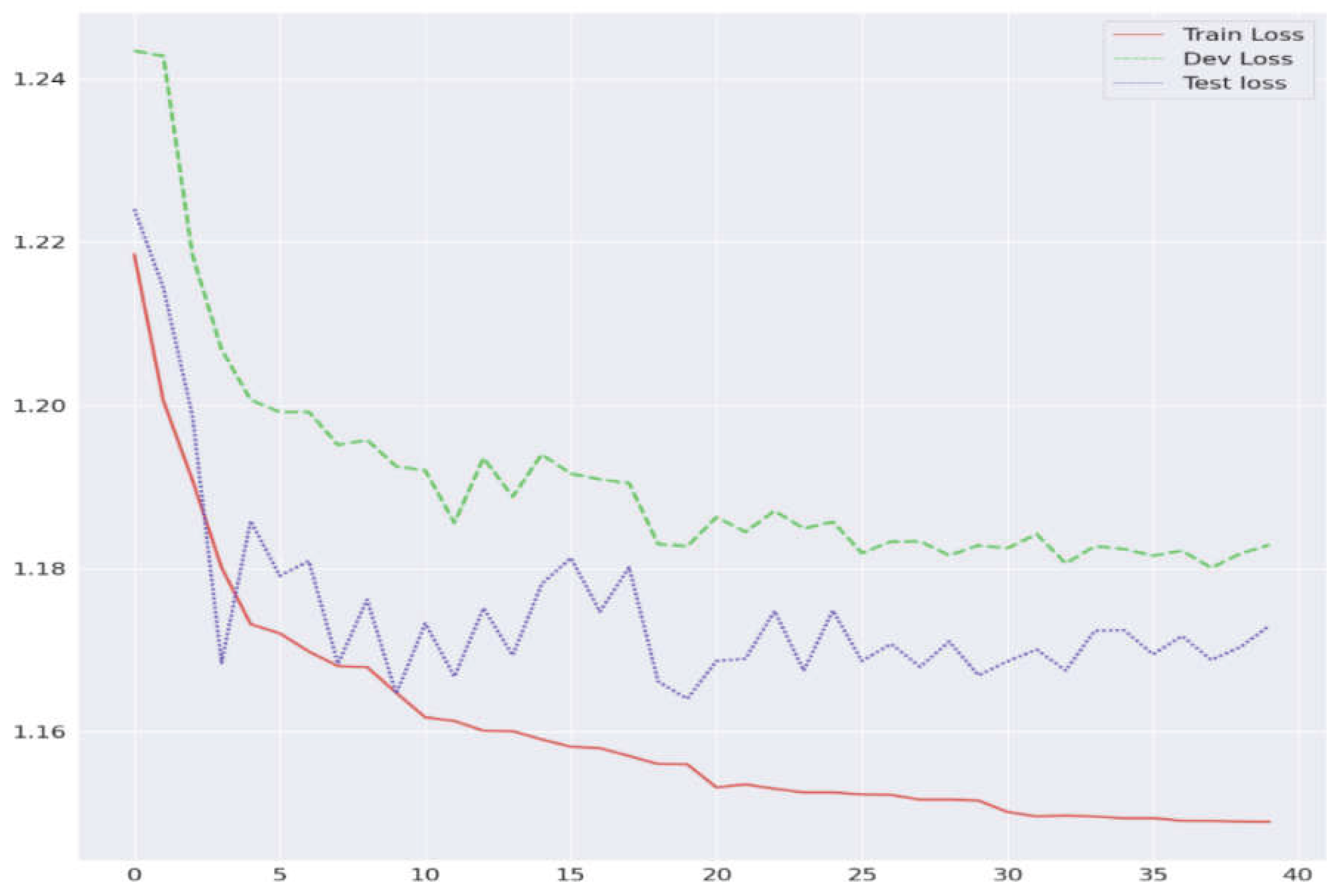
Figure 3.
Results for weak and semi-strong market efficiency.
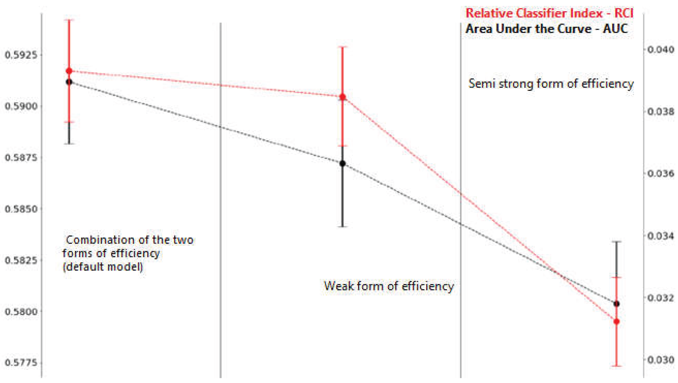
Figure 4.
Time-varying market efficiency.
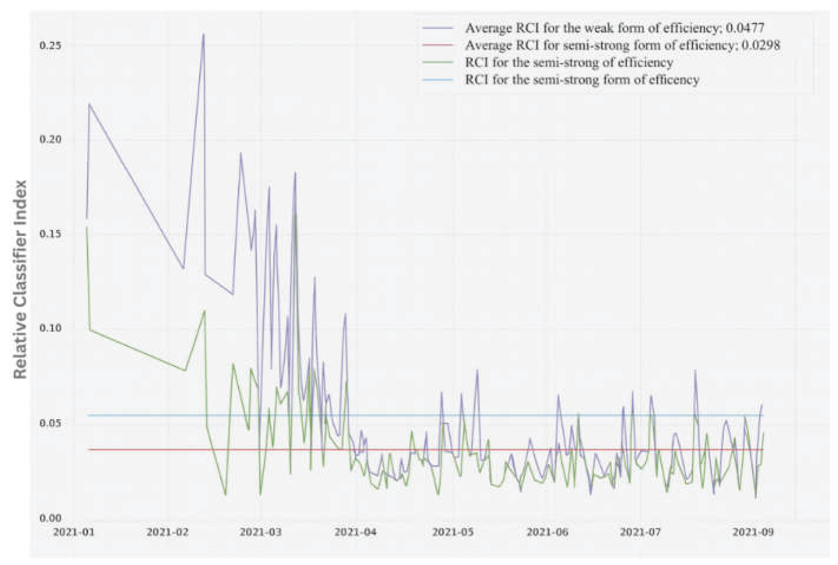
Figure 5.
Price memory limit over time.
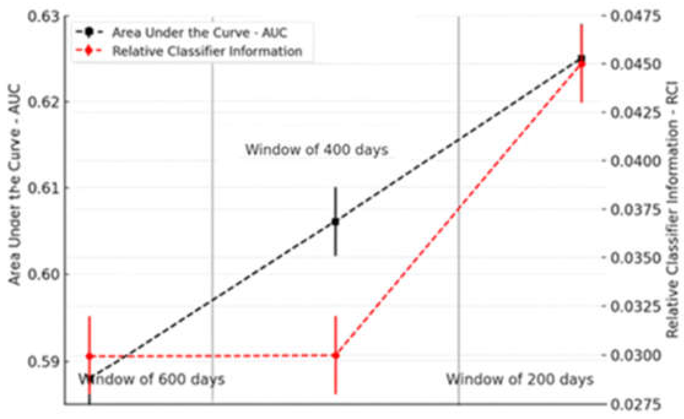

Table 1.
GRU-D Model performance.
| Metric | Average | Lower limit | Upper limit |
|---|---|---|---|
| at 99.99% | at 99.99% | ||
| Micro-Average AUC | 74.62% | 74.54% | 74.71% |
| Class 1 - AUC | 68.43% | 68.15% | 68.70% |
| Class 2 - AUC | 54.80% | 54.62% | 54.98% |
| Class 3 - AUC | 58.43% | 58.04% | 58.83% |
| Class 4 - AUC | 55.01% | 54.82% | 55.19% |
Table 2.
RCI across sub-samples.
| Sub-samples | Mean | Standard Deviation | Min | 25% | 50% | 75% | Max | |
|---|---|---|---|---|---|---|---|---|
| Weak form of efficiency | Countries sub-samples | 2.2% | 1.9% | 0.01% | 0.08% | 0.26% | 0.26% | 0.86% |
| Sectors sub-samples | 2.6% | 0.26% | 0.01% | 0.09% | 0.17% | 0.34% | 1.39% | |
| Semi-strong form of efficiency | Countries sub-samples | 1.6% | 0.15% | 0.01% | 0.09% | 0.13% | 0.18% | 0.69% |
| Sectors sub-samples | 2.3% | 0.23% | 0.01% | 0.07% | 0.16% | 0.28% | 1.09% |
Disclaimer/Publisher’s Note: The statements, opinions and data contained in all publications are solely those of the individual author(s) and contributor(s) and not of MDPI and/or the editor(s). MDPI and/or the editor(s) disclaim responsibility for any injury to people or property resulting from any ideas, methods, instructions or products referred to in the content. |
© 2026 by the authors. Licensee MDPI, Basel, Switzerland. This article is an open access article distributed under the terms and conditions of the Creative Commons Attribution (CC BY) license (http://creativecommons.org/licenses/by/4.0/).
Copyright: This open access article is published under a Creative Commons CC BY 4.0 license, which permit the free download, distribution, and reuse, provided that the author and preprint are cited in any reuse.


