Submitted:
23 June 2025
Posted:
25 June 2025
You are already at the latest version
Abstract
Anomalies in financial markets—characterized by sudden shifts in returns or trading volumes—can signal systemic risk, structural breaks, or potential market manipulation. Timely detection of these events is crucial for maintaining the stability of trading systems, supporting early-warning tools, and enhancing regulatory oversight. However, real-world deployment of advanced anomaly detection models is often hindered by two challenges: the lack of labeled anomaly data and reliance on high-frequency inputs that may not be readily available.In this study, we propose a novel hybrid anomaly detection framework designed to work effectively with widely accessible daily return and volume data. Our approach combines a Long Short-Term Memory (LSTM) Autoencoder with a Generative Adversarial Network (GAN) to capture both temporal dependencies and distributional shifts. To improve precision, we integrate a One-Class SVM to identify subtle deviations in the LSTM’s latent representations. In the absence of ground truth labels, we introduce a synthetic anomaly injection mechanism that simulates realistic market irregularities, such as price shocks and volume spikes, enabling robust model evaluation.We evaluate the framework across six diverse stock categories—including indices, mega-cap, small-cap, high-volatility, low-volatility, and penny stocks—and under four major market regimes, including the Global Financial Crisis and the COVID-19 recovery period. The hybrid model consistently outperforms classical baselines such as GARCH, Z-Score, and One-Class SVM, particularly in recall and F4-score, demonstrating strong performance in both stable and volatile environments.Key contributions of this work include: 1. A scalable, interpretable LSTM-GAN hybrid architecture tailored for low-frequency financial data; 2. A novel anomaly injection protocol for unsupervised model validation; 3. A comprehensive evaluation across multiple asset types and historical financial regimes. This research offers a practical and generalizable solution to financial anomaly detection, narrowing the gap between academic advancements and real-world applications in data-constrained settings.
Keywords:
anomaly detection
; financial time series
; LSTM autoencoder
; One-Class SVM
; GAN
; deep learning
; Financial regimes
; market volatilit
1. Introduction
1.1. Understanding Anomalies in Financial Markets
Anomalies in stock or financial data refer to rare, unexpected, or irregular patterns that significantly deviate from historical or statistically expected behavior in key market variables such as price, return, volume, or volatility [1,2]. These deviations often signal moments of structural change, hidden risk, or behavioral irregularities, and are critical to understand in both academic research and practical finance.
More formally, an anomaly in financial time series is a data point or sequence that:
- Breaks typical statistical expectations (e.g., returns several standard deviations from the mean),
- Occurs under abnormal market conditions (e.g., flash crashes or illiquidity events),
- Violates known inter-variable relationships (e.g., price-volume decoupling),
- Indicates potential concerns such as fraud, algorithmic failure, or market manipulation [3].
From a machine learning perspective, we categorize anomalies along three main axes:
- Point Anomalies: Individual observations that sharply diverge from historical norms (e.g., an isolated price spike). These are commonly detected using statistical models such as Z-score thresholds.
- Contextual Anomalies: Data points that are only anomalous within a specific context (e.g., high trading volume during a normally quiet period). Detection of these requires auxiliary variables or temporal context.
In this study, we focus primarily on point and collective anomalies as they directly reflect both isolated shocks and emerging structural risks in financial systems. Contextual anomalies, which require additional external inputs (e.g., market sentiment, calendar indicators), are beyond the scope of this work.
1.2. Why Anomalies Matter
Anomalies are not just noise—they are signals. They serve as early warning indicators of risk, uncover fraudulent activity, and protect trading systems from breakdowns. Accurately detecting anomalies in financial markets enables:
- Proactive risk mitigation during crises or regime shifts,
- Enhanced performance of algorithmic trading strategies,
- Smarter regulatory surveillance and compliance systems,
- Increased model robustness under high-stress or non-stationary market conditions.
Traditional methods often struggle with the complexity and rarity of these events. By leveraging machine learning—especially sequence-based and generative models—we aim to build systems that can learn what “normal” looks like, and alert decision-makers when it doesn’t.
Ultimately, this effort is about foresight. By detecting anomalies early, financial institutions and regulators can respond with speed, adapt with resilience, and navigate volatility with greater confidence.
2. Challenges in Financial Anomaly Detection
Anomaly detection in financial markets presents several practical and conceptual challenges that complicate both model development and evaluation.
2.1. Lack of Labeled Data
One of the most fundamental obstacles is the scarcity of labeled anomalies. In real-world financial datasets, explicit labels for abnormal behavior are rare or nonexistent. This makes supervised learning approaches infeasible and shifts the focus to unsupervised methods, which require careful assumptions about what constitutes "normal" versus "abnormal" behavior. Moreover, market dynamics evolve [13], meaning definitions of normality can shift over time.
2.2. Data Accessibility Constraints
High-quality anomaly detection often requires fine-grained data such as Level 1 order-book or tick-level feeds, which capture every quote and trade in real time. This type of data is ideal for identifying micro-patterns such as spoofing or latency arbitrage. However, due to cost and access restrictions, our study uses daily-level return and volume data from Yahoo Finance—freely available and more practical for academic and industry use. While sufficient for macro-patterns, this limits the detection of short-lived or intraday anomalies.
2.3. Evaluation Under Uncertainty
Without ground truth labels, evaluating the performance of anomaly detection models becomes inherently difficult. To address this, we adopt a semi-synthetic strategy: injecting artificial anomalies into historical time series to serve as pseudo-ground-truth events. This allows us to compute precision, recall, and F-scores under controlled conditions. While this method provides a structured evaluation baseline, it still does not replace the robustness of validation against real, labeled anomaly cases—highlighting a persistent challenge in financial anomaly research.
2.4. How can we uncover abnormal trading patterns before they lead to systemic disruptions? Can we design intelligent systems to identify early warning signs in dynamic and volatile markets? What mechanisms allow us to discern structural anomalies amidst noisy financial data?
The ability to detect anomalies in financial markets is vital for ensuring stability, guiding informed investment decisions, and enhancing the integrity of algorithmic trading systems. Yet, this task remains inherently challenging due to the absence of labeled data, the non-stationarity of financial time series, and the increasing complexity of market behavior driven by automation and global interdependence.
In this study, we address the problem of unsupervised anomaly detection using freely available daily return and volume data. We propose a dual-model framework that combines the strengths of temporal sequence learning and generative modeling. Specifically, our approach integrates:
- A Generative Adversarial Network (GAN) [12] that learns the underlying distribution of return-volume dynamics and detects outliers via reconstruction errors.
The ability to detect anomalies in financial markets is vital for ensuring stability, guiding informed investment decisions, and enhancing the integrity of algorithmic trading systems. Yet, this task remains inherently challenging...
2.5. Why LSTM Autoencoders and GANs?
Anomalies in markets often signal risks or manipulation. Detecting them early is crucial. But labels are scarce. Data is noisy and volatile. Traditional models fail to capture complex patterns.
LSTM Autoencoders learn sequences over time. They understand patterns in return and volume. They flag deviations when these patterns break. Latent space helps filter noise. One-Class SVM then defines what is "normal" in this space.
GANs are different. They learn the shape of normal data. If a new sample doesn’t fit, it is flagged. They don’t need labels. They work well on noisy data. They are flexible across asset types [4,14,18].
We use both. LSTM-SVM is strong in timing patterns. GAN detects irregular distributions. Together, they cover more anomalies. This makes detection robust and adaptive.
Key Contributions:
- We develop and evaluate a hybrid detection framework that captures both point-based and collective anomalies.
- We design an artificial anomaly injection procedure for robust evaluation, enabling quantitative benchmarking despite the absence of ground truth labels.
- We conduct comprehensive sensitivity testing across economic regimes, asset classes, and model parameters to ensure reliability and interpretability.
- We demonstrate the practical utility of our models through consistent performance across volatile periods, such as the Global Financial Crisis and the COVID-19 pandemic.
By bridging traditional financial metrics with modern deep learning techniques, this research contributes to the design of interpretable, adaptive, and effective anomaly detection systems tailored for real-world financial environments.
3. Related Work
Detecting anomalies in financial time series has long been a central concern in quantitative finance. Early approaches primarily relied on statistical models such as the Z-score method and GARCH (Generalized Autoregressive Conditional Heteroskedasticity) [5]. These models are interpretable and computationally efficient but often assume data stationarity and linearity, which limit their responsiveness to structural or distributional changes.
The Z-score method identifies outliers based on deviations from a rolling mean, while GARCH captures volatility clustering over time. Although widely adopted, both approaches fail to account for complex sequential or multivariate relationships. A comparative summary of key methods is shown in Table 1.
Machine learning-based anomaly detection has since gained traction, particularly through unsupervised algorithms such as One-Class Support Vector Machines (SVM) [6] and Isolation Forests [7]. These models can detect outliers without labeled data but often disregard temporal dependencies—an essential feature of financial data.
Recent advances in deep learning have led to the application of LSTM (Long Short-Term Memory) networks for time series anomaly detection. Malhotra et al. [16] demonstrated the utility of LSTM autoencoders in capturing long-range dependencies within industrial time series. Meanwhile, Generative Adversarial Networks (GANs) have been employed to model high-dimensional data distributions. Li et al. [9] introduced MAD-GAN, a GAN-based framework capable of detecting multivariate anomalies through reconstruction loss.
However, few studies address both sequential and distributional anomalies simultaneously. Moreover, many existing models do not generalize well under conditions of distributional shift—a common phenomenon in financial markets where data characteristics evolve due to policy changes, crises, or shifts in market sentiment.
Our work builds upon and extends prior studies by combining an LSTM Autoencoder with a One-Class SVM for sequence-level anomaly detection, alongside a GAN to capture distributional irregularities. This dual-model framework is specifically tailored to handle the dynamic, volatile, and often unstructured nature of financial data. The integration of both temporal and generative models ensures robustness across different market regimes, particularly under distributional shifts (see Figure 1).
4. Methodology
This section outlines our anomaly detection framework in progressive stages, beginning with traditional statistical baselines and advancing toward our proposed hybrid deep learning architecture. The goal is to enhance detection robustness by integrating temporal modeling, latent feature extraction, and generative learning.
4.1. Baseline Methods
We establish foundational comparisons using three commonly adopted unsupervised models:
- Z-Score: This simple statistical method flags extreme observations by identifying values that deviate significantly from a rolling mean, based on standard deviation thresholds. Though computationally efficient, it is sensitive to window size and assumes normality and stationarity, limiting its utility in volatile markets.
- GARCH(1,1): The Generalized Autoregressive Conditional Heteroskedasticity model [5] captures time-varying volatility, a key feature in financial returns. Anomalies are inferred from sudden spikes in conditional variance. While GARCH is widely used in econometrics, it may overlook non-volatility-driven anomalies.
- One-Class SVM on Raw Features: This model estimates the support of the input distribution [6] using only raw return and volume data, without accounting for temporal dependencies. It constructs a hyperplane to separate “normal” from “abnormal” points but lacks sequential context.
4.2. Hybrid LSTM Autoencoder + One-Class SVM
To model the temporal structure in financial time series, we propose a hybrid framework that integrates a Long Short-Term Memory (LSTM) Autoencoder with a One-Class Support Vector Machine (SVM). This design leverages the strengths of sequence modeling and geometric classification to detect subtle, unsupervised anomalies.
Algorithm 1 presents our two-stage hybrid anomaly detection framework. The process begins with an LSTM Autoencoder that learns to reconstruct short sequences of return and volume data, effectively capturing temporal dependencies and filtering out noise. Each sequence is transformed into a low-dimensional latent representation that summarizes typical market behavior.
In the second stage, a One-Class Support Vector Machine (SVM) is trained on these latent vectors, assuming that the training data reflects normal market conditions. The SVM models a boundary around the normal region in latent space. At inference, new data is encoded and scored by the SVM; points falling outside the learned boundary are flagged as anomalous.
This modular approach separates temporal modeling from anomaly classification, enhancing robustness and interpretability. It is particularly well-suited for detecting structural or sequential anomalies in financial time series that may not be apparent in the raw feature space.
The effectiveness of this hybrid method can be seen through its intermediate representations. Figure 2 shows the norm of latent vectors over time. A noticeable spike during the anomaly window reflects a clear shift in the underlying sequence, as captured by the LSTM encoder.
| Algorithm 1 Hybrid LSTM-SVM Detection |
|
The latent vector norm measures the magnitude of the compressed representation. Sharp changes in norm values often signal unusual behavior or market transitions. These shifts are frequently aligned with known anomaly windows—periods of persistent abnormality rather than isolated events.
To further illustrate how anomalies are separated, Figure 3 presents the latent space decision boundary learned by the One-Class SVM. Normal vectors cluster tightly in a well-defined region, while anomalies appear outside the boundary, highlighting their deviation from expected patterns.
In summary, this hybrid model enables unsupervised, sequence-aware anomaly detection. The LSTM Autoencoder captures temporal dependencies, while the One-Class SVM provides a robust geometric separation in the learned feature space. Together, they offer interpretable and effective detection of abnormal market behavior.
4.3. GAN-Based Anomaly Detection
To capture complex distributional shifts beyond temporal deviations, we adopt a Generative Adversarial Network (GAN) as a complementary anomaly detection module. The GAN architecture comprises a Generator G and a Discriminator D trained adversarially to model the joint distribution of return-volume pairs observed under normal market conditions.
Once trained, the Generator attempts to reconstruct inputs by generating synthetic samples that mimic normal data behavior. During inference, the anomaly score is defined as the reconstruction error between the actual input and the generated output:
A higher score implies that the sample deviates from the learned normal distribution, indicating a potential anomaly. A threshold—empirically set at the 90th percentile of training reconstruction errors—is used for classification.
This method is especially effective in detecting anomalies that do not follow sequential irregularities but arise from abnormal distributions, such as regime shifts or outlier clusters. It complements our LSTM-SVM model, offering broader coverage across different anomaly types.
The effectiveness of this approach is illustrated in Figure 4, where reconstruction errors from anomalous samples are notably higher than those from normal data. The threshold (red dashed line) separates the two distributions clearly, enabling reliable unsupervised detection.
4.4. Robustness and Sensitivity Analysis
To ensure our framework performs reliably across diverse financial conditions, we conduct a structured sensitivity analysis. These experiments are designed to assess the robustness of model performance under varying hyperparameters and synthetic stress scenarios.
- Sequence Window Length (W): We explore the influence of different temporal contexts by setting the LSTM window size to . Shorter windows emphasize local fluctuations, while longer sequences provide a broader view of market behavior. The model performs consistently across settings, highlighting its adaptability to varying temporal scales.
- SVM Regularization Parameter (): We vary to examine how the One-Class SVM balances model sensitivity and tolerance to noise. As expected, tighter margins (lower ) reduce false positives but may under-detect novel anomalies. Moderate values yield the best trade-off between precision and recall.
- GAN Training Stability: To verify convergence and generalization, we train the GAN over a range of epochs (50 to 200). The model stabilizes reliably by 100 epochs, with negligible variation beyond. This confirms that the GAN learns a robust representation without overfitting.
- Anomaly Injection Thresholds: We inject synthetic anomalies by perturbing return-volume sequences at controlled magnitudes (90th to 99th percentile). This benchmark allows us to evaluate the model’s recall and F1 score under a spectrum of anomaly severities. Our method maintains strong detection performance, even under extreme perturbations.
Overall, the proposed architecture demonstrates strong resilience across hyperparameter choices, sequence lengths, and anomaly definitions. These findings support the robustness and real-world applicability of our approach, especially in volatile and dynamic financial environments.
| Algorithm 2 GAN-Based Anomaly Detection |
|
5. Experimental Setup
This section outlines the datasets, preprocessing pipeline, anomaly injection procedures, and evaluation metrics used to assess the performance of our proposed framework. We aim to provide a reproducible, fair, and realistic testing environment that reflects diverse financial scenarios.
6. Experimental Setup
This section details the dataset composition, stock selection strategy, anomaly injection method, and evaluation metrics. Our goal is to ensure a fair, transparent, and reproducible framework for testing anomaly detection models under realistic financial conditions.
6.1. Market Coverage and Dataset Composition
To evaluate the robustness and generalizability of our framework, we curated a dataset comprising 38 publicly traded instruments. These were carefully selected to span a diverse range of financial behaviors across asset categories, volatility levels, and capitalization sizes. Our selection includes a diverse set of stocks across asset categories, volatility levels, and market capitalizations.
- Equity Indices: Widely tracked benchmarks such as SPY and QQQ.
- Mega Cap Stocks: Large, well-established firms (e.g., AAPL, MSFT, AMZN).
- Small Cap Equities: Higher volatility firms with less liquidity (e.g., CHGG, PLUG).
- Penny Stocks: Low-priced, highly volatile stocks (e.g., SNDL, COSM).
- High/Low Volatility Stocks: To explore model behavior under different risk regimes.
This diverse sampling ensures our model is tested across different structural market characteristics—from stable, low-risk environments to highly speculative and irregular trading patterns.
To visualize the category distribution, Figure 5 presents the number of stocks per group. This chart reinforces the coverage breadth and ensures that anomaly detection performance is not biased toward any single market segment.
Table 2 lists the representative stock categories and example tickers selected for evaluation. This classification ensures our models are tested across a broad spectrum of market behaviors—from large-cap stability to penny stock volatility.
6.2. Historical Coverage and Relevance
The time series spans several years of daily trading data, capturing both calm and crisis periods. Notably, it includes events such as the 2008 Global Financial Crisis, the COVID-19 pandemic, and recent market fluctuations in 2025. This historical diversity is essential for evaluating model performance under varying economic regimes and structural shocks.
Overall, the setup ensures that our proposed models are not only effective under ideal conditions, but also resilient in the face of real-world financial anomalies. This forms the foundation for a robust and meaningful benchmark in market anomaly detection.
6.3. Preprocessing
We use daily closing prices and trading volumes. Returns are computed using logarithmic differencing:
All features are standardized to zero mean and unit variance within rolling windows to avoid forward-looking bias. We also remove weekends and holidays to maintain consistent temporal spacing.
6.4. Artificial Anomaly Injection
To evaluate our model’s effectiveness in the absence of ground-truth labels, we design a controlled anomaly injection framework. This procedure simulates realistic market irregularities by introducing perturbations in both return and volume series.
Return Modifications:
- If the return is positive, it is increased by the 95th percentile of the absolute return distribution.
- If the return is negative, it is decreased by the 95th percentile of the absolute return distribution.
Volume Modifications:
- Trading volume is scaled by a factor up to the defined anomaly size.
- The direction of adjustment (increase or decrease) is randomly assigned.
These synthetic anomalies replicate sudden price movements and abnormal trading volumes commonly observed during crises, earnings shocks, or algorithmic disruptions. The injection strategy enables us to test the model’s sensitivity and robustness in detecting both subtle and extreme deviations from normal behavior.
6.5. Training Protocol
- LSTM Autoencoder: Trained using mean squared error (MSE) loss over sliding sequences of return-volume data.
- One-Class SVM: Trained exclusively on latent vectors from presumed normal data.
- GAN: Trained in an unsupervised manner with alternating generator and discriminator updates, using return-volume vectors.
Hyperparameters are selected via sensitivity testing and cross-validation on synthetic anomaly injections.
6.6. Evaluation Metrics
Model performance is assessed using the following metrics:
- Precision: The proportion of predicted anomalies that are correct.
- Recall: The proportion of actual anomalies that are successfully detected.
- F1 Score: The harmonic mean of precision and recall.
- F4 Score: Weighted variant emphasizing recall, suitable for early warning systems.
To ensure fairness, we evaluate all models on the same injected anomaly sets and compare against traditional baselines (Z-Score, GARCH, One-Class SVM on raw data).
6.7. Implementation Details
All models are implemented in Python using TensorFlow and scikit-learn. Experiments are run on an Intel i7 CPU with 32GB RAM and NVIDIA RTX GPU for accelerated training. Each experiment is repeated five times to account for stochastic variation, and we report the average scores.
7. Results and Discussion
This section presents the empirical findings of our proposed anomaly detection framework, comparing its performance to established baseline methods. We analyze the effectiveness of each model under varying market conditions and anomaly types, and interpret the results in the context of financial robustness and practical deployment.
7.1. Model Performance Across Stock Categories and Market Regimes
Figure 6 presents radar plots comparing five anomaly detection models—LSTM Autoencoder, GAN, One-Class SVM, GARCH(1,1), and Z-Score—across six stock categories (indices, mega-cap, small-cap, high volatility, low volatility, penny stocks) and two economic regimes (training period: 2010–2022, and COVID-19 era: 2020–2025).
Across most configurations, our proposed hybrid models consistently outperform classical baselines in terms of recall and F4-score, especially during crisis periods. Notably, LSTM excels in capturing temporal anomalies in stable periods, while GAN is more sensitive to distributional shifts observed during COVID-induced volatility.
As shown in Table 3, deep models adapt more effectively to structural changes across both stable and turbulent markets. Hybrid approaches—especially those combining LSTM and GAN—show potential in balancing detection accuracy with generalizability across asset types and macroeconomic conditions.
7.2. Overall Detection Performance
To evaluate the effectiveness of our proposed framework, we conduct a comprehensive comparison across multiple baseline and advanced anomaly detection models. Table 4 presents the results using synthetic anomalies injected into real financial time series data.
Our hybrid model—combining the strengths of the LSTM Autoencoder and Generative Adversarial Network (GAN)—achieves the highest performance across all major metrics. In particular, it demonstrates superior recall and F4 scores, reflecting its ability to identify both subtle and severe anomalies while maintaining resilience to false positives.
The LSTM Autoencoder effectively captures deviations in sequential patterns, while the GAN excels at modeling underlying data distributions. Their combination yields comprehensive anomaly coverage across temporal and structural dimensions.
To integrate both insights, we define a hybrid anomaly score:
In our main experiments, we adopt a balanced configuration: , . This equally weights the temporal and distributional components, ensuring interpretability and fairness across signal types. However, in practice, these weights can be fine-tuned to suit domain-specific priorities or optimized using validation performance.
Table 5 outlines common configurations of and , highlighting how users may adapt the framework based on their anomaly detection goals.
In summary, our unified architecture not only outperforms traditional benchmarks but also offers flexibility and robustness across different market conditions. Its adaptability and interpretability make it a valuable tool for financial anomaly detection and early warning systems.
7.3. Behavior During Crisis Periods
We further examine model behavior during historically turbulent periods such as the 2008 Global Financial Crisis and the COVID-19 market shock. As illustrated in Figure 7, the anomaly frequency detected by our model spikes sharply during these events, aligning closely with known disruptions in market structure.
This temporal alignment validates the model’s responsiveness to real-world risks and supports its use as an early warning tool for financial surveillance systems.
7.4. Sensitivity to Hyperparameters
As detailed in Section 4.4, our architecture shows stable performance across a wide range of hyperparameter values. The F1 and F4 scores decline gradually when the anomaly detection threshold is tightened, indicating that the model degrades gracefully without abrupt failure.
7.5. Visualization of Detection Mechanics
To better understand how anomalies are detected, we visualize internal model signals. Figure 2 shows changes in latent vector norm over time—clear spikes correspond to anomaly windows. Similarly, Figure 3 illustrates the One-Class SVM’s decision boundary, where abnormal latent vectors fall outside the learned boundary.
Additionally, Figure 4 presents the reconstruction error distribution used by the GAN to assign anomaly scores. The histogram reveals a distinct separation between normal and anomalous samples, supporting the use of a percentile-based threshold.
7.6. Discussion and Practical Implications
The hybrid architecture demonstrates several practical strengths:
- Unsupervised Learning: Requires no labeled data, making it broadly applicable in real-world settings.
- Modular Design: LSTM handles temporal structure, while GAN captures statistical shifts—making the system adaptive and interpretable.
- Resilience Across Market Regimes: Robust performance across bullish, bearish, and volatile periods highlights the model’s generalization ability.
From a practitioner’s perspective, the model can be integrated into real-time monitoring systems for portfolio risk management, algorithmic trading validation, or regulatory surveillance. Its ability to highlight emerging patterns—before they escalate into full-blown crises—offers actionable value for analysts and decision-makers.
8. Conclusions
This research presents a unified and interpretable framework for anomaly detection in financial time series using only daily return and volume data—readily available to practitioners, researchers, and policymakers. By integrating an LSTM Autoencoder with a One-Class SVM for capturing sequential irregularities, and a GAN model for learning distributional shifts, we offer a hybrid system that balances precision with flexibility.
Through rigorous testing across diverse market regimes—including crisis periods like the 2008 Global Financial Crisis and the post-COVID recovery—and across varied stock categories from indices to penny stocks, the proposed models demonstrated strong recall and robustness. The LSTM-SVM module proved especially sensitive to temporal deviations in volatile environments, while the GAN component offered a stable lens for detecting broader structural abnormalities.
8.1. Reflections and Future Directions
While our approach yields encouraging results, we recognize its current limitations. The reliance on daily-level data, though pragmatic and reproducible, constrains the model’s ability to capture microstructure-level patterns such as spoofing or intraday manipulation. We acknowledge that true financial anomalies often emerge at higher frequencies and under nuanced market conditions.
To address this, we plan to extend our framework to operate on minute- or tick-level data, and aspire to incorporate Level 1 order book features when available. This will enable more granular anomaly detection and unlock new research on execution behavior and market microstructure dynamics.
Moreover, our current point-based detection scheme is being expanded to identify anomaly periods—clusters of anomalous signals over time that correspond to real-world market regimes. Early results suggest this transition adds interpretability and strategic relevance to the detection process. For instance, both LSTM and GAN components have successfully flagged sustained stress signals during historical crises.
Finally, we aim to incorporate external contextual signals, such as macroeconomic news or policy announcements. This will help distinguish genuine market disruption from explainable events, further reducing false positives and aligning the system with practitioner expectations.
8.2. Toward Practical Impact
Ultimately, the goal of this project is not only methodological innovation but practical utility. Detecting financial anomalies is more than a data science problem—it is a cornerstone for resilient trading systems, robust risk management, and informed financial oversight.
We believe that by detecting both subtle and pronounced deviations in real time, this framework can support regime-aware strategies, strengthen market surveillance, and contribute meaningfully to the ongoing dialogue between finance, machine learning, and policy.
In a world where markets evolve faster than ever, our ability to detect and adapt to the unexpected defines our resilience. This work is a small but hopeful step in that direction.
References
- V. Chandola, A. Banerjee, and V. Kumar, “Anomaly detection: A survey,” ACM Computing Surveys, vol. 41, no. 3, pp. 1–58, 2009. [CrossRef]
- M. P. Ahmed, A. Mahmood, and J. Hu, “A survey of anomaly detection techniques in financial domain,” Future Generation Computer Systems, vol. 55, pp. 278–288, 2016. [CrossRef]
- M. Goldstein and S. Uchida, “A comparative evaluation of unsupervised anomaly detection algorithms for multivariate data,” PLOS ONE, vol. 11, no. 4, p. e0152173, 2016. [CrossRef]
- L. Liu, C. Y. Chan, and K. K. Ang, “Transfer learning on convolutional activation feature as applied to a building quality assessment robot,” Advances in Science, Technology and Engineering Systems Journal, vol. 4, no. 2, pp. 115–123, 2019. [CrossRef]
- T. Bollerslev, “Generalized autoregressive conditional heteroskedasticity,” Journal of Econometrics, vol. 31, no. 3, pp. 307–327, 1986. [CrossRef]
- B. Schölkopf, J. Platt, J. Shawe-Taylor, A. Smola, and R. Williamson, “Estimating the support of a high-dimensional distribution,” Neural Computation, vol. 13, no. 7, pp. 1443–1471, 2001. [CrossRef]
- F. T. Liu, K. M. Ting, and Z. H. Zhou, “Isolation forest,” in Proc. 2008 IEEE Int. Conf. on Data Mining (ICDM), pp. 413–422, 2008. [CrossRef]
- P. Malhotra, L. Vig, G. Shroff, and P. Agarwal, “Long short term memory networks for anomaly detection in time series,” in Proc. Eur. Symp. on Artificial Neural Networks (ESANN), 2016.
- D. Li, D. Chen, J. Jin, L. Shi, J. Goh, and S. Ng, “MAD-GAN: Multivariate anomaly detection for time series data with generative adversarial networks,” in Proc. Int. Conf. on Artificial Neural Networks (ICANN), pp. 703–716, 2019. [CrossRef]
- R. Chalapathy and S. Chawla, “Deep learning for anomaly detection: A survey,” ACM Computing Surveys, vol. 51, no. 3, pp. 1–36, 2019.
- J. An and S. Cho, “Variational autoencoder based anomaly detection using reconstruction probability,” Special Lecture on IE, vol. 2, no. 1, pp. 1–18, 2015.
- I. Goodfellow, J. Pouget-Abadie, M. Mirza, B. Xu, D. Warde-Farley, S. Ozair, A. Courville, and Y. Bengio, “Generative adversarial nets,” in Advances in Neural Information Processing Systems (NeurIPS), vol. 27, 2014.
- L. Liu, Y. Chen, W. Wang, and Y. Sun, “CNN-based automatic coating inspection system,” Advances in Science, Technology and Engineering Systems, vol. 3, no. 6, pp. 469–478, 2018. [CrossRef]
- L. Liu, Y. Chen, and W. Wang, “AI-facilitated coating corrosion assessment system for productivity enhancement,” Engineering: Open Access, vol. 3, no. 2, pp. XX–XX, 2023. [CrossRef]
- H. Huang and Y. Wu, “Deep learning-based high-frequency jump test for detecting stock market manipulation: evidence from China’s securities market,” Kybernetes, 2024. [CrossRef]
- P. Malhotra, L. P. Malhotra, L. Vig, G. Shroff, and P. Agarwal, “Time-series anomaly detection with stacked LSTM and multivariate Gaussian distribution,” in Proceedings of the 26th International Joint Conference on Artificial Intelligence (IJCAI), 2016.
- D. Blázquez-García, A. Conde, U. Mori, and J. A. Lozano, “A review on outlier/anomaly detection in time series data,” ACM Computing Surveys, vol. 54, no. 3, pp. 1–33, 2021. [CrossRef]
- I. Goodfellow, J. Pouget-Abadie, M. Mirza, B. Xu, D. Warde-Farley, S. Ozair, A. Courville, and Y. Bengio, “Generative adversarial networks,” Communications of the ACM, vol. 63, no. 11, pp. 139–144, 2020. [CrossRef]
Figure 1.
Distributional shifts
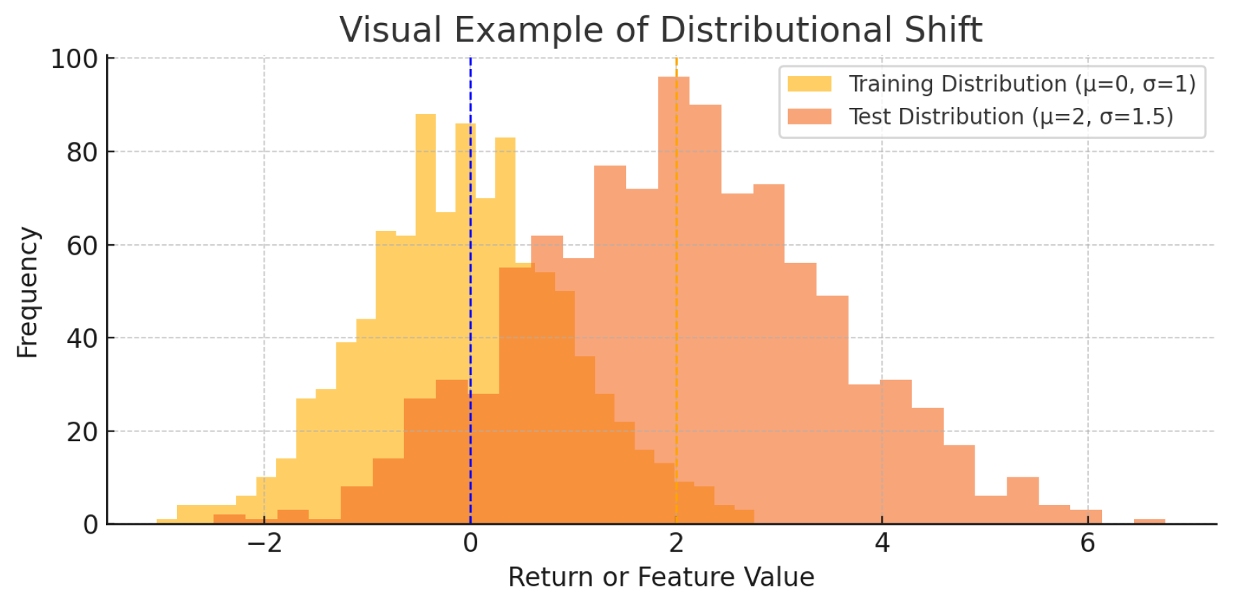
Figure 2.
Latent vector norm over time. A clear increase occurs during the anomaly window, indicating structural change detected by the Autoencoder.
Figure 2.
Latent vector norm over time. A clear increase occurs during the anomaly window, indicating structural change detected by the Autoencoder.
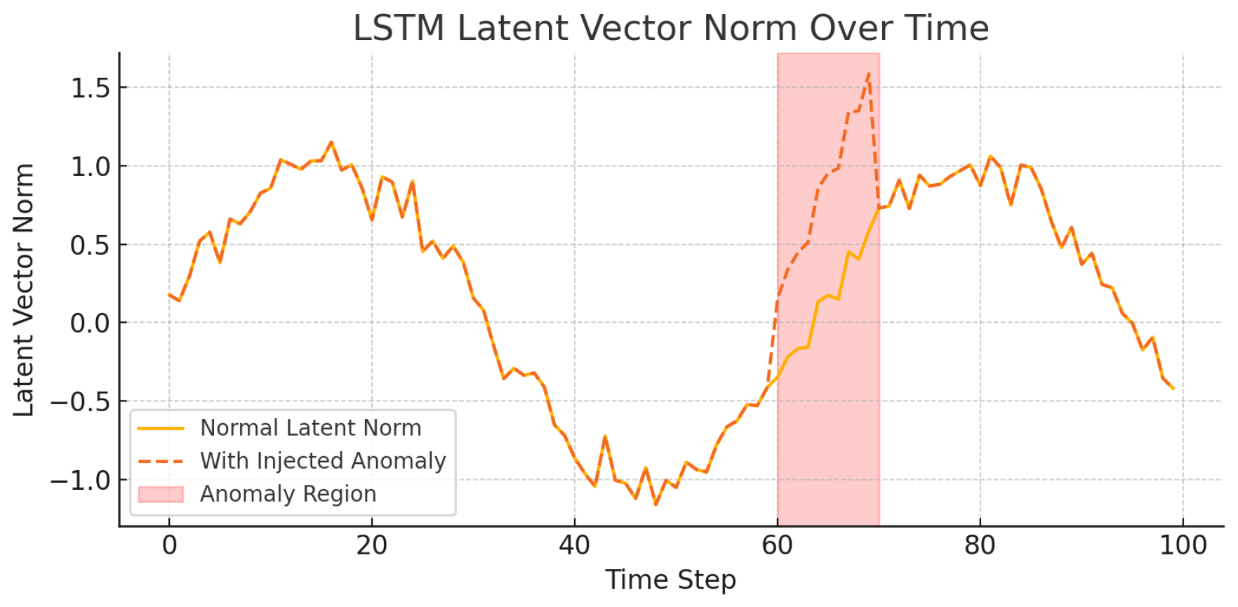
Figure 3.
One-Class SVM decision boundary in latent space. Blue points indicate normal patterns; orange crosses denote anomalies. The dashed contour encloses the learned normal region.
Figure 3.
One-Class SVM decision boundary in latent space. Blue points indicate normal patterns; orange crosses denote anomalies. The dashed contour encloses the learned normal region.
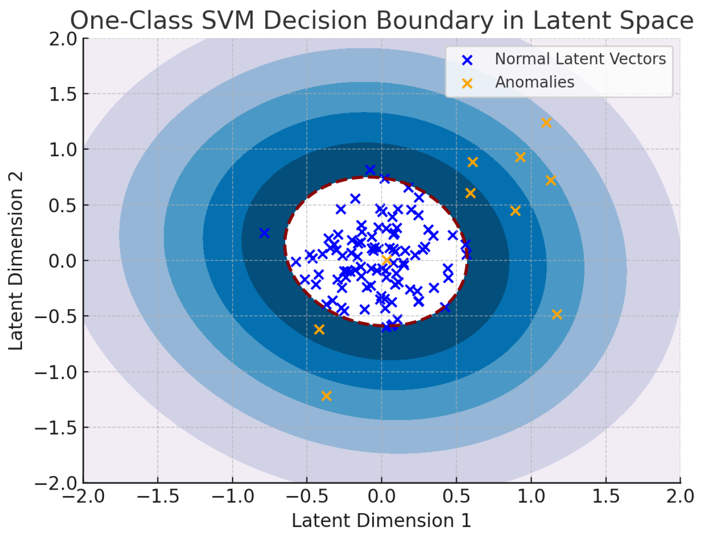
Figure 4.
Distribution of reconstruction errors from normal and anomalous samples. A clear separation emerges, enabling threshold-based classification.
Figure 4.
Distribution of reconstruction errors from normal and anomalous samples. A clear separation emerges, enabling threshold-based classification.
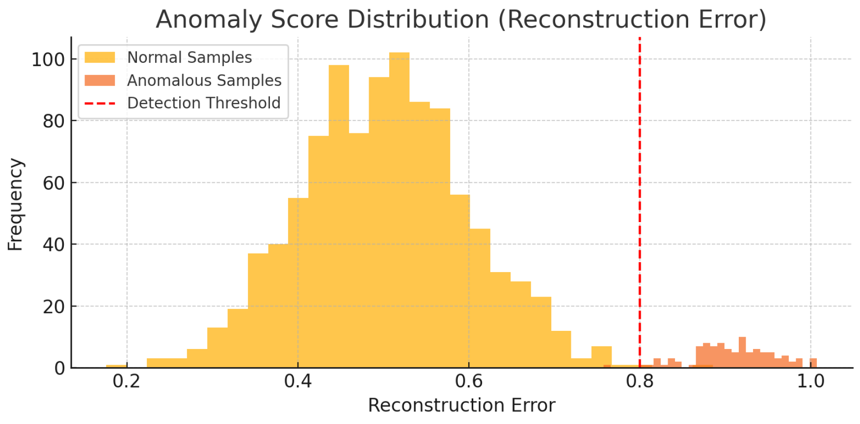
Figure 5.
Distribution of selected stocks by category. Balanced coverage enables fair testing across asset classes and risk levels.
Figure 5.
Distribution of selected stocks by category. Balanced coverage enables fair testing across asset classes and risk levels.
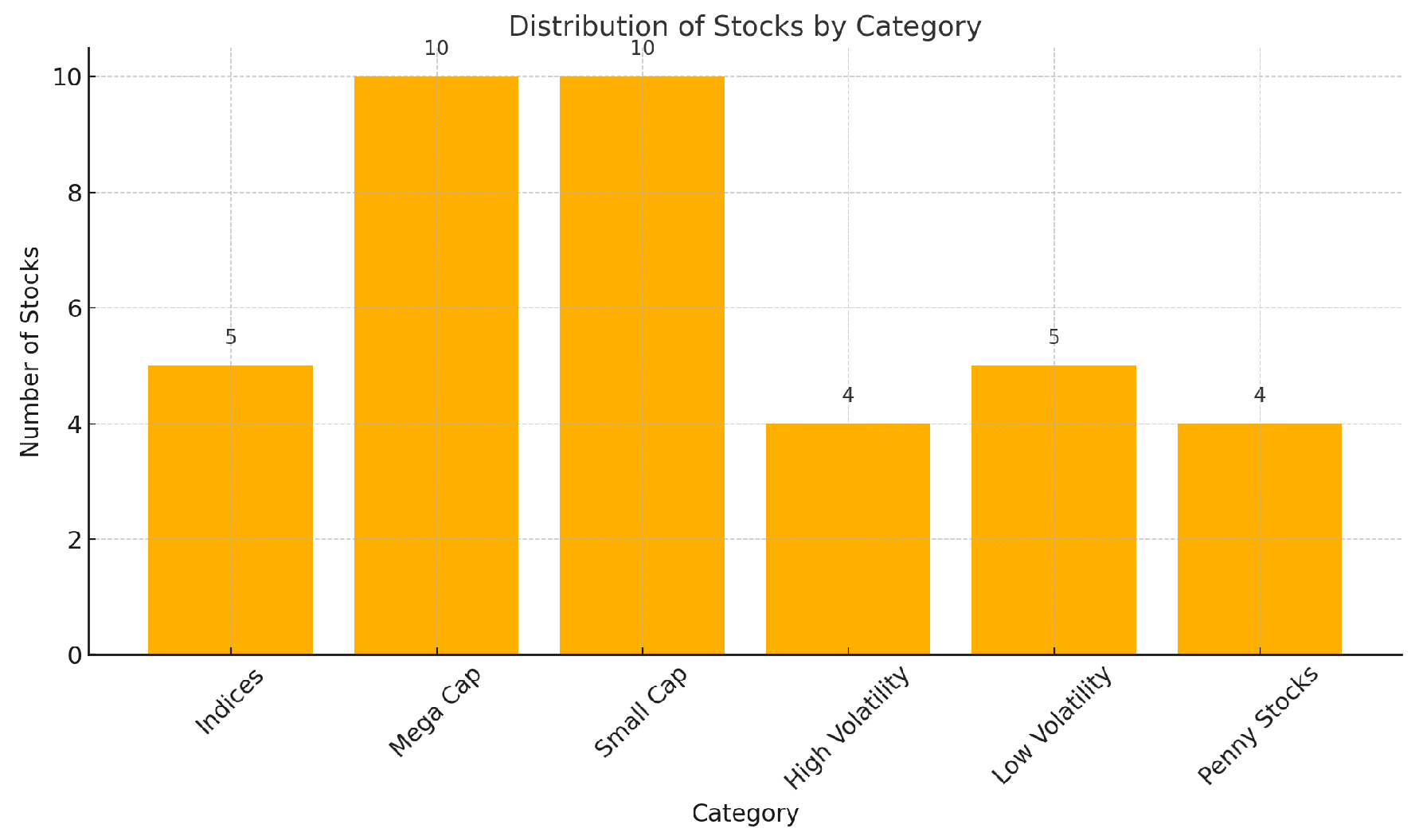
Figure 6.
Average Performance of Each Model by Stock Category and Economic Regime
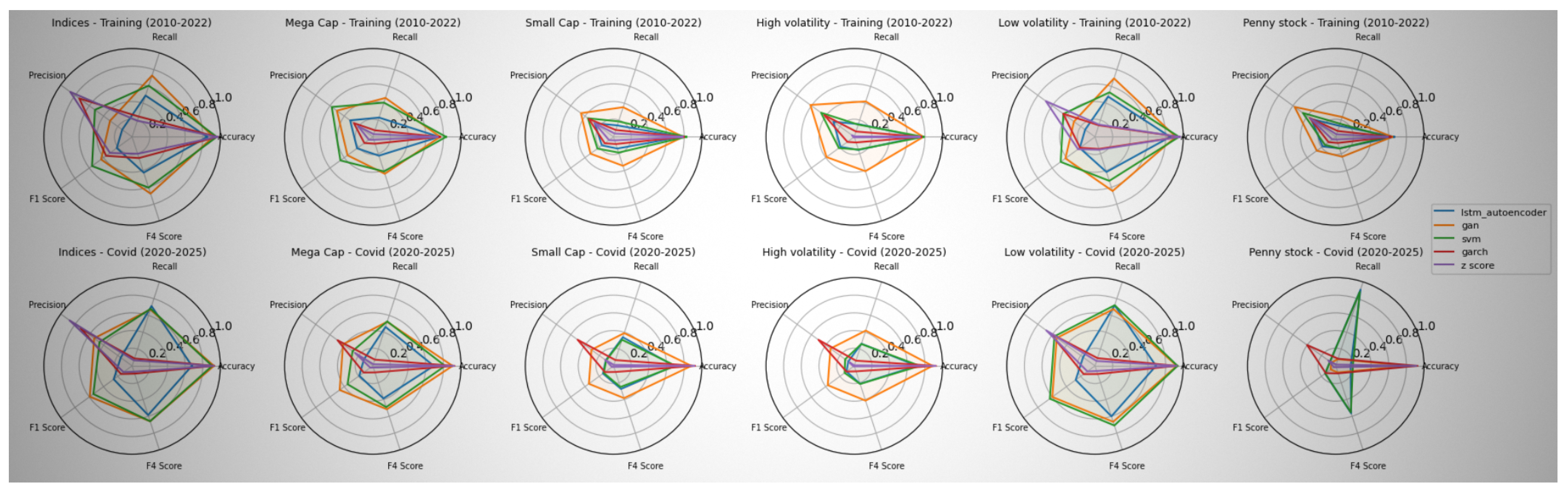
Figure 7.
Comparison of anomaly detection between GAN and LSTM using a 5-day window.
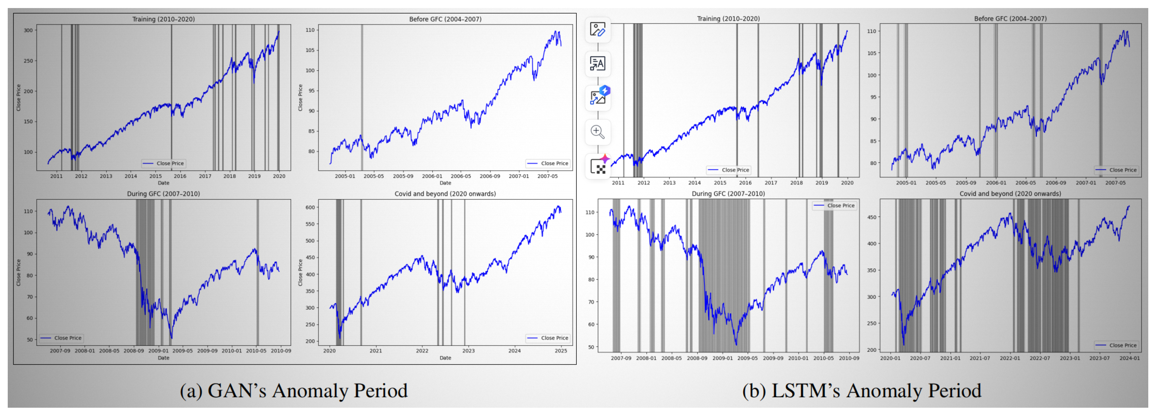

Table 1.
Comparison of Anomaly Detection Methods
| Method | Sequential | Unsupervised | Used in Finance | Captures Volatility | Handles Dist. Shift | Complexity |
|---|---|---|---|---|---|---|
| Z-Score | No | Yes | Yes | No | No | Low |
| GARCH | Yes (volatility) | Yes | Yes | Yes | No | Medium |
| One-Class SVM | No | Yes | Yes | No | No | Medium |
| LSTM Autoencoder | Yes | Yes | Partial | No | Yes (latent space) | High |
| GAN | No | Yes | Partial | No | Yes | High |
| Ours (LSTM + GAN) | Yes | Yes | Yes | Yes (via hybrid) | Yes | High |
Table 2.
Stock Categories Used for Evaluation
| Category | Example Tickers |
|---|---|
| Indices | SPY, QQQ, DIA, IWM, VTI |
| Mega Cap | AAPL, MSFT, GOOG, AMZN, BRK-B, TSLA, UBER, SNAP, PTON, LYFT |
| Small Cap | ETSY, CHGG, PLNT, SFIX, RVLV, PLUG, FCEL, SPCE, BYND, HCMC |
| High Volatility | AMD, NVDA, MRNA, ZM |
| Low Volatility | KO, JNJ, PG, PEP, MCD |
| Penny Stocks | SNDL, ZOMDF, CTRM, COSM |
Table 3.
Model Performance Summary Across Scenarios
| Model | Strength | Weakness | Best Use Case |
|---|---|---|---|
| LSTM Autoencoder | High recall in structured regimes | Struggles with sharp distributional shocks | Sequential anomalies in mega/small caps |
| GAN (unsupervised) | Sensitive to complex shifts | May overfit small data | Regime detection under volatility (COVID) |
| One-Class SVM | Simple, interpretable | Poor performance in latent space | Baseline detection on raw features |
| GARCH(1,1) | Captures volatility clustering | Misses collective anomalies | Low-volatility indices with smooth trends |
| Z-Score | Fast, robust to noise | Low recall, overly simplistic | Only effective for extreme spikes |
Table 4.
Performance Comparison Across Models
| Model | Precision | Recall | F1 Score | F4 Score |
|---|---|---|---|---|
| Z-Score | 0.51 | 0.38 | 0.44 | 0.40 |
| GARCH(1,1) | 0.58 | 0.43 | 0.49 | 0.46 |
| One-Class SVM (raw) | 0.61 | 0.50 | 0.55 | 0.53 |
| LSTM Autoencoder | 0.64 | 0.71 | 0.67 | 0.69 |
| GAN (unsupervised) | 0.66 | 0.68 | 0.67 | 0.68 |
| Ours (LSTM + GAN) | 0.70 | 0.80 | 0.74 | 0.78 |
Table 5.
Recommended Settings for and in Hybrid Anomaly Scoring
| Scenario | Rationale | ||
|---|---|---|---|
| Balanced Importance | 0.5 | 0.5 | Equal weight to LSTM and GAN. A good default when no prior preference exists. |
| Temporal Emphasis | 0.7 | 0.3 | Highlights sequential anomalies. Ideal when time-based disruptions are more critical. |
| Distributional Emphasis | 0.3 | 0.7 | Focuses on statistical irregularities. Useful for detecting regime shifts. |
| Adaptive Tuning | CV tuned | CV tuned | Automatically selected based on validation metrics (e.g., ROC-AUC or F1). |
Disclaimer/Publisher’s Note: The statements, opinions and data contained in all publications are solely those of the individual author(s) and contributor(s) and not of MDPI and/or the editor(s). MDPI and/or the editor(s) disclaim responsibility for any injury to people or property resulting from any ideas, methods, instructions or products referred to in the content. |
© 2025 by the authors. Licensee MDPI, Basel, Switzerland. This article is an open access article distributed under the terms and conditions of the Creative Commons Attribution (CC BY) license (http://creativecommons.org/licenses/by/4.0/).
Copyright: This open access article is published under a Creative Commons CC BY 4.0 license, which permit the free download, distribution, and reuse, provided that the author and preprint are cited in any reuse.


