Submitted:
30 December 2025
Posted:
31 December 2025
You are already at the latest version
Abstract
Non-line-of-sight (NLOS) propagation poses a significant challenge to achieving high-accuracy ultra-wideband (UWB) indoor positioning. To address this issue, this study investigates solutions from two complementary perspectives: NLOS identification and error mitigation. First, an NLOS signal classification model is proposed based on multidimensional statistics of the channel impulse response (CIR). The model incorporates an attention mechanism and an improved snake optimization (ISO) algorithm, achieving significantly enhanced classification accuracy and robustness. Building on this foundation, a UKF–BiLSTM dual-directional mutual calibration framework is proposed to compensate for NLOS errors dynamically. The framework embeds the constant turn rate and velocity (CTRV) motion model within an unscented Kalman filter (UKF) to enhance trajectory modeling. It establishes a bidirectional correction loop with a bidirectional long short-term memory (BiLSTM) network. Through the synergy of physical constraints and data-driven learning, the framework adaptively suppresses NLOS errors. Experimental results demonstrate that the proposed classification model and positioning framework significantly outperform state-of-the-art methods, thereby providing a systematic solution for high-precision and robust UWB positioning in complex indoor environments.
Keywords:
ultra-wideband(UWB)
; non-line-of-sight(NLOS)
; unscented Kalman filter (UKF)
; bidirectional long short-term memory(BiLSTM)
; indoor positioning
1. Introduction
In indoor environments, Global Positioning System (GPS) signals are often unavailable or unreliable. Consequently, a variety of indoor positioning technologies have been developed, including Wi-Fi [1], Bluetooth [2], ZigBee[3], and ultra-wideband (UWB) [4]. Among these technologies, UWB offers high data rates, low power consumption, and acceptable time-domain resolution, making it particularly suitable for high-precision indoor positioning. As a result, UWB has been widely applied in practical scenarios such as industrial monitoring [5] and drone positioning[6].
However, in practical indoor environments, UWB positioning systems are inevitably affected by non-line-of-sight (NLOS) propagation. When obstacles block the direct path between the transmitter and receiver, signals propagate through reflected or diffracted paths, leading to increased propagation time and positively biased ranging errors [7]. These NLOS-induced errors significantly degrade positioning accuracy and may even result in positioning failure in complex scenarios, thereby limiting the overall performance of UWB-based indoor positioning systems. Therefore, effective identification of NLOS conditions and suppression of their adverse effects are critical for improving the accuracy of UWB indoor positioning.
To address this challenge, recent studies have explored the integration of deep learning techniques with traditional filtering algorithms to mitigate NLOS errors. Tian et al. [8] proposed a KF–LSTM framework, in which Kalman filtering (KF) constrains physical-state estimation while a long short-term memory (LSTM) network models measurement errors, thereby demonstrating the feasibility of such hybrid approaches. Eang et al. [9] developed a deep neural network (DNN)–extended Kalman filter (EKF) fusion framework in which a neural network estimates ranging biases and the EKF subsequently updates the state. Zhou et al. [10] further proposed a CNN–LSTM–DEKF method, in which a cascaded CNN–LSTM architecture is employed for NLOS identification, and the resulting classification information is incorporated into a distributed EKF (DEKF) to enable high-precision positioning under specific scenarios. To relax the limitations imposed by linear assumptions, Zhang et al. [11] designed a UKF–FNN–RIC framework. By integrating a feedforward neural network (FNN) with a redundant information correction (RIC) mechanism, the proposed framework enables progressive coupling with nonlinear physical models. As a result, millimeter- and centimeter-level accuracy can be achieved for static positioning and simple trajectory-tracking tasks. Overall, these studies represent essential advances in fusion-based NLOS mitigation; however, two fundamental limitations remain. First, KF/EKF/DEKF-based approaches rely on linearization assumptions, which make them difficult to generalize to complex dynamic scenarios with highly nonlinear motion characteristics. Second, although UKF-based nonlinear frameworks alleviate linearity constraints, most of them adopt a unidirectional fusion paradigm and lack dynamic bidirectional feedback between physical models and deep learning components, limiting their adaptability to complex, time-varying environments.
To overcome these limitations and achieve effective integration of physical constraints and data-driven learning, this paper proposes a unified framework that jointly addresses NLOS identification and NLOS error mitigation. The main contributions are summarized as follows:
- 1)
- An enhanced classification model is proposed by integrating multi-head self-attention with an improved snake optimization (ISO) algorithm. The self-attention mechanism captures correlations among channel impulse response (CIR) features, while the optimization strategy adaptively searches for optimal network parameters, thereby improving classification accuracy and model robustness.
- 2)
- A UKF–BiLSTM model with a bidirectional mutual calibration mechanism is proposed for NLOS error mitigation. The constant turn rate and velocity (CTRV) motion model is adopted to enhance the trajectory modeling capability of the UKF. Specifically, the UKF provides physically constrained and optimized initial estimates for the bidirectional LSTM (BiLSTM), while the BiLSTM learns from historical residuals to dynamically adjust the UKF’s measurement noise statistics. This bidirectional interaction enables adaptive suppression of NLOS-induced errors under complex and time-varying conditions.
2. Related Work
2.1. Physics-Based Methods
In physical model-based UWB positioning research, filtering methods have long played a dominant role. Among these, the KF—one of the earliest dynamic estimation frameworks—assumes linear-Gaussian distributions and is therefore ill-suited for nonlinear ranging processes in complex indoor environments [12]. To address such nonlinearity, the EKF has been widely adopted by applying first-order linearization to nonlinear systems; however, such linearization inevitably introduces limitations, particularly for nonlinear ranging models in complex environments [13,14]. To overcome these drawbacks, the unscented Kalman filter (UKF) employs the unscented transformation (UT), which avoids explicit Jacobian calculations and often provides improved performance in nonlinear systems. In addition to these filtering methods, optimization-based enhancements have been developed to improve robustness. For example, Lyu et al. [15] combined an improved particle swarm optimization (IPSO) algorithm with an adaptive UKF that updates the noise covariance matrix in real time to mitigate NLOS errors. Likewise, Feng et al. [16] developed an EKF–UKF fusion framework that integrates improved ranging techniques with geometric dilution of precision (DOP) optimization, enabling complementary updates from multiple information sources. In parallel, particle filtering (PF)—a representative nonparametric Bayesian estimation method—naturally handles nonlinear and non-Gaussian noise and has been widely applied to UWB indoor positioning [17]. As an example, Han et al. [18] proposed an adaptive ant colony optimization particle filter (AACOPF) for joint estimation of position and heading for a single mobile node, combining IMU/UWB fusion with dynamic weight adjustment. Despite these advances, most existing methods assume that auxiliary nodes are in motion; when such nodes are static, the system may become unobservable, thereby limiting practical applicability. In summary, filtering-based approaches offer strong interpretability and real-time performance, but their effectiveness depends heavily on predefined physical and noise models. In complex NLOS environments, modeling non-Gaussian and time-varying error characteristics remains challenging, and filtering-based methods often struggle to capture long-term temporal dependencies. These limitations have motivated increasing interest in data-driven approaches.
2.2. Deep Learning-Based NLOS Mitigation
Early studies primarily explored the application of CNNs and LSTM networks to UWB positioning, which evolved along two distinct technical pathways. For temporal modeling, Poulose et al. [19] employed a two-layer LSTM network to process time-of-arrival (TOA) ranging sequences. They achieved a mean positioning error of 7 cm in indoor line-of-sight (LOS) simulation scenarios. This result highlighted the potential of deep learning for modeling dynamic trajectories. However, the method is limited to ideal LOS conditions and requires a relatively long training time. From a feature representation perspective, Nguyen et al. [20] converted UWB signals into three-channel RGB images and employed CNNs for end-to-end localization. This approach achieved meter-level accuracy across multiple channel models. Nevertheless, it relies heavily on high signal-to-noise ratios, shows markedly increased errors in complex scenarios such as suburban NLOS environments, and incurs relatively high inference latency. In summary, these pioneering studies demonstrated the potential of temporal and feature-based learning for UWB positioning. They also revealed fundamental limitations of early deep learning approaches, notably their heavy reliance on simulated data and ideal operating conditions. To address these limitations, subsequent research has shifted toward network architectures that explicitly model the geometric structure inherent in localization tasks. He et al. [21] introduced a spatio-temporal graph neural network (STA-GNN) framework for UWB positioning. This framework explicitly models the geometric topological relationships between anchors and tags. In real indoor environments, their framework achieved positioning errors of 4.7-22.4 cm. By leveraging efficient graph convolution operations, it attained a real-time positioning frequency of 10 Hz on embedded platforms. Although the aforementioned CNN- and LSTM-based methods can achieve millisecond-level inference in simulation environments, STA-GNN is among the first to show that deep learning–based localization can satisfy system-level real-time requirements in complex real-world scenarios. This advancement marks a transition from algorithm-level validation in simulation toward practical system-level deployment. Building on the success of Transformer architectures in sequence modeling, researchers have applied attention mechanisms to improve both the accuracy and robustness of UWB positioning. Tang et al. [22] proposed a deep attention network that integrates a Transformer encoder with a GRU module. They also introduced a geometric loss function to enforce sensor constraints. In real-world complex scenarios, this approach reduces ranging errors to approximately 0.1–0.2 m and achieves single-sample inference in just 0.004 seconds. This provides a favorable balance between accuracy and efficiency. However, its performance is highly scenario-specific, requiring retraining when anchor layouts change, and thus it suffers from limited transferability. To enhance environmental adaptability, subsequent efforts have focused on the tight integration of Transformers with domain knowledge. Yang et al. [23] further proposed the F-BERT framework, which deepens this integration by combining Transformers with fuzzy logic for fine-grained distance correction. The framework achieves centimeter-level positioning accuracy in dynamic NLOS scenarios. It experiences only a 6.56% performance drop across different environments, demonstrating strong adaptability and robustness. In summary, deep learning continues to push the boundaries of accuracy through architectural innovations. However, its purely data-driven nature presents two fundamental limitations. First, model predictions lack guidance from physical kinematic constraints, leading to non-physical outputs in complex dynamic trajectories. Second, performance heavily depends on the distribution of the training data, limiting cross-scenario generalization. Therefore, the tight integration of data-driven learning with physical model constraints has emerged as a critical pathway for further advances in performance and robustness.
2.3. Hybrid Model-Based NLOS Mitigation
To address the respective limitations of model-driven and data-driven approaches, hybrid paradigms that integrate their complementary strengths have become a central focus in high-precision UWB positioning research. Existing studies can be broadly categorized by the degree of integration, revealing a progression from simple combinations to deeply collaborative frameworks. Early studies predominantly adopted unidirectional, open-loop fusion strategies. For instance, Tian et al. [8] employed a KF as a pre-processing stage for an LSTM network to denoise input measurements. This strategy improves positioning accuracy in ideal LOS scenarios; however, because there is no interaction between the filtering module and the neural network, the network exhibits limited adaptability in complex, dynamic NLOS environments. To further mitigate multi-source errors, subsequent research evolved toward multi-stage, cascaded fusion architectures. Zhang et al. [11] proposed a cascaded combination of a UKF, an FNN, and an RIC module, while Wang et al. [24] extended this framework by embedding the Chan algorithm between the FNN and RIC modules. This design stabilizes the conversion of time-difference-of-arrival (TDOA) measurements into absolute distances, mitigating the instability inherent to conventional implicit-function solutions. Such frameworks sequentially address random and systematic errors through multiple specialized modules during geometric optimization, achieving millimeter- to centimeter-level positioning accuracy in static and low-speed dynamic scenarios. Nonetheless, their performance remains highly dependent on predefined processing pipelines, and the complex serial structure often incurs significant computational overhead. More recently, research has shifted toward end-to-end, physically-informed architectures that explicitly reflect the underlying physics of localization. A representative approach enhances key components of physical filters using deep learning networks. For example, Ren et al. [25] employed an attention-enhanced LSTM network to generate pseudo-observations for the KF under NLOS conditions, thereby incorporating data-driven information into the state estimation process. Another approach reconstructs the entire system using network architectures aligned with physical relationships. Muthineni et al. [26] adopted graph neural networks (GNNs) to model anchors and tags as nodes in a graph. Through message passing, multimodal data are naturally fused while geometric constraints among sensors are explicitly encoded. Nevertheless, the mechanisms for collaboration remain inherently constrained. Attention-based LSTM methods still act as unidirectional substitutes for physical filters. In contrast, end-to-end architectures such as GNNs do not integrate a concurrently operating physical state estimator to provide real-time physical constraints and corrective feedback.
In summary, although existing hybrid methods have improved accuracy and robustness, they generally lack adaptive interaction mechanisms between physical and data-driven modules, and thus fail to form a unified closed-loop optimization framework. To address this gap, this paper proposes a novel fusion framework for state estimation that enables real-time, closed-loop integration of physical constraints and data-driven learning.
3. NLOS Identification Model
3.1. Analysis of Parameters Related to NLOS Recognition
Feature extraction was conducted on CIR waveforms to enable NLOS identification. Based on the DW1000 User Manual [27], basic features were selected, including first-path amplitudes (FP_AMP1–FP_AMP3), noise statistics (Stdev_Noise, Max_Noise), and channel impulse response power (CIR_PWR). To optimize the input and improve model efficiency, a random forest (RF) was additionally employed to assess feature importance, from which the top 10 features were selected as the final input. This screening process improves the discriminative power of the features while reducing dimensionality, providing a basis for subsequent recognition models.
Figure 1 compares CIR waveforms under LOS and NLOS conditions. The LOS CIR waveform exhibits notably higher peaks, reflecting stronger signal strength and faster energy decay. In contrast, the NLOS CIR waveform has lower peaks and longer, more gradual tails. In LOS environments, signals travel along relatively direct paths, encountering minimal obstacles and incurring minimal energy loss. In contrast, NLOS signals propagate along complex paths that involve reflections and refractions, leading to substantial energy loss and the formation of multipath components. These distinct waveform characteristics provide the physical basis for extracting discriminative statistical features from the CIR.
Figure 2 shows box plots of FP_AMP1, FP_AMP2, and FP_AMP3, illustrating the distributions of first-path amplitude parameters under LOS and NLOS conditions. Analyzing differences in signal amplitude allows for a more accurate determination of whether a signal propagates under LOS or NLOS conditions, thereby assisting in assessing the signal’s environment. Figure 2(a) and 2(c) show higher medians and more concentrated distributions under LOS conditions, indicating that the first-path amplitude is higher and more stable. In contrast, Figure 2(b) shows outliers under LOS conditions, possibly due to signal amplification caused by environmental reflections or scattering. Overall, the three figures indicate that signal amplitudes are generally higher under LOS conditions, with lower attenuation, while NLOS signals are more affected by multipath propagation. These distribution differences suggest that the first-path amplitude is an effective feature for distinguishing LOS and NLOS channels, and it is incorporated into the feature set for model training.
Figure 3 shows box plots of the maximum noise value and the noise standard deviation. Figure 3(a) presents the maximum noise values, which are overall lower in NLOS environments. The median is significantly smaller than that under LOS conditions, and the interquartile range is narrow, indicating limited variability. In contrast, under LOS conditions, the maximum noise level exhibits a higher median and a broader distribution, with a markedly extended upper tail and higher extreme values. This reflects greater instability and a wider dynamic range of maximum noise under LOS conditions. Figure 3(b) shows the noise standard deviation, whose median is significantly higher in the NLOS group than in the LOS group. In addition, the interquartile range is broader and more outliers are observed, indicating increased noise variability and instability in NLOS environments. This behavior arises from the pronounced multipath delay spread in NLOS channels, where signals from different paths interfere with one another, leading to highly dispersed noise statistics in the time domain. In contrast, noise sources in LOS channels are less diverse, resulting in more stable statistical characteristics. Therefore, the noise standard deviation serves as an effective auxiliary indicator for assessing multipath dominance, providing an additional statistical basis for LOS/NLOS identification.
Figure 4 shows the box plot of channel impulse response power (CIR_PWR). Under LOS conditions, the CIR_PWR distribution exhibits a higher median, a narrower interquartile range, and shorter whiskers, indicating stronger and more stable signal power.
The above analysis demonstrates significant differences between LOS and NLOS channels in time-domain amplitude, noise statistics, and energy distribution. These distinctions constitute the physical basis for feature selection. Accordingly, ten of the most discriminative features are selected from the original CIR, reducing the input dimensionality while preserving key information. These features serve as optimized inputs for the recognition model described in Section 3.3.
3.2. Snake Optimizer
The snake optimizer (SO) is a novel metaheuristic optimization algorithm proposed by Fatma A. Hashim and Abdelazim G. Hussien in 2022 [28]. The algorithm simulates the foraging and reproductive behaviors of snakes in nature and formulates these behaviors into an optimization process through mathematical modeling, enabling the solution of diverse optimization problems. The core mechanism of the snake optimizer relies on a dynamic temperature threshold to distinguish between two primary behavioral modes: global exploration (foraging) and local exploitation (mating). During initialization, a population of snakes is randomly generated, where each individual represents a candidate solution. The population is then ranked according to fitness and evenly divided into a male group and a female group .
In each iteration, the environmental temperature and the food quantity act as two key control variables. The temperature follows a simulated exponential cooling schedule, expressed as, where denotes the current iteration index and represents the maximum number of iterations.
The food quantity is defined as the ratio between the current best fitness value and the worst fitness value, serving as an indicator of food abundance within the search space:
where and represent the best and worst fitness values within the current population, respectively.
When the temperature is low, the algorithm enters the exploration phase. This phase simulates the foraging behavior of a snake population, where movement strategies are further determined by the food availability . If food is scarce , an individual snake tends to perform a global random walk:
where denotes the position vector of a randomly selected individual within the population, is a random number uniformly distributed in the interval , and is a predefined attack intensity constant that controls the step size of the random walk. When food is abundant, snakes move toward the known optimal food source position (i.e., the position vector corresponding to the individual with the best fitness in the current population):
The factor here serves to regulate the step size; the lower the temperature, the stronger the certainty of movement toward the food source.
When the environmental temperature is suitable , the algorithm switches to the exploitation phase, simulating mating and competitive behaviors among snakes. During this phase, male and female groups operate independently. Male individuals enter a combat mode, in which they move toward the current optimal male (i.e., the position vector of the individual with the best fitness within the male group ), while simultaneously experiencing competitive interference from a randomly selected male (i.e., a randomly chosen position vector within the group ):
Meanwhile, when food is abundant and the random mating condition is satisfied, a female individual (a randomly selected position vector from the female group ) interacts with a selected male individual (a randomly selected position vector from the male group ), producing an offspring position , which is computed as the average of the two:
Newly generated offspring replace the worst individuals in the current population, thereby maintaining population size and introducing new search potential. After each position update, the algorithm performs boundary checks and applies a greedy selection mechanism to retain superior solutions, guiding the population toward the global optimum. Through dual regulation of temperature and food quantity, combined with dynamic switching between exploration and exploitation behaviors, the Snake Optimizer achieves efficient and adaptive search within the solution space.
3.3. ISO-MBP Model
To enhance the recognition accuracy of NLOS states in complex indoor UWB scenarios, this paper proposes an NLOS recognition model that integrates an ISO algorithm with a multi-head backpropagation network (MBP). The overall model consists of three stages: feature representation and initial classification based on BP–multi-head self-attention (MHSA, stage A); an ISO incorporating iterative chaotic map with infinite collapses (ICMIC) chaotic mapping and differential evolution (DE) mechanisms (stage B); and global optimization of BP network parameters using ISO (stage C).
In Phase A, the input feature vector of each sample is denoted as , where represents the dimensionality of the input features. The BP neural network first applies a linear transformation followed by a nonlinear activation to the input features, and the output of the first hidden layer is given by:
where and denote the weight matrix and bias vector of the first hidden layer, respectively. represents the number of neurons in the hidden layer, and denotes the ReLU activation function.
To enhance the model’s capability to capture correlations across different feature subspaces, an MHSA mechanism is introduced after the first hidden layer. This mechanism operates on the feature representation space rather than on temporal modeling. To improve feature propagation stability and accelerate convergence, residual connections and layer normalization are incorporated into the attention module. The hidden layer output is treated as a single-step feature embedding, and its Query, Key, and Value vectors are defined as follows:
among these, , , and are learnable projection matrices. Within a single attention head, the scaled dot-product attention is computed as follows:
where denotes the dimensionality of the key vector. Multi-head attention constructs attention heads in parallel to model the input representation across different feature subspaces, yielding the following output:
where denotes the output projection matrix.
Subsequently, the attention-enhanced feature representations are fed into the subsequent hidden layers, with the computation performed as follows:
where and denote the weight matrix and bias vector of the second hidden layer, respectively. Finally, the output layer produces the classification result for each sample:
where and represent the weight matrix and bias vector of the output layer, respectively. During model training, the cross-entropy loss function is employed as the objective function to quantify the discrepancy between the predicted results and the ground-truth labels.
Phase B addresses the issues of uneven initial population distribution and premature convergence that often occur in traditional SO algorithms within high-dimensional search spaces. Improvements are introduced by incorporating the ICMIC chaotic mapping and DE mechanisms. First, the ICMIC chaotic mapping is employed to generate the initial snake population, mathematically expressed as:
where denotes the initial position of the snake individual, and represent the lower and upper bounds of the search space, respectively, denotes the element-wise product, and is the chaotic sequence vector. The chaotic sequence is generated using the following mapping:
where denotes the predefined chaotic constant.
During the iteration process, DE operators are applied to perturb and update individuals in the snake swarm. The mutation operation is expressed as:
where , and are distinct random indices, and is the predefined constant for differential mutation. Candidate solutions are generated through crossover operations and then selected for update based on the fitness function, thereby enhancing the algorithm’s global search capability and maintaining population diversity.
In Phase C, all weights and bias parameters in the BP neural network are uniformly flattened and encoded into a one-dimensional parameter vector:
where denotes the vectorization operation, which expands matrices column-wise into one-dimensional vectors. The ISO algorithm employs the classification loss on the BP neural network’s training set as the fitness function:
where denotes the fitness function during the optimization process, and represents the cross-entropy loss function.
Through continuous updates of individual snakes within the search space, the global optimal parameters are ultimately obtained:
These parameters are then used as the initial values for the BP neural network in subsequent training, effectively integrating global search capabilities with local gradient-based learning. This integration significantly enhances both the classification performance and the robustness of the NLOS recognition model.
4. NLOS Error Mitigation Model
4.1. CTRV Model
The CTRV model is a widely adopted kinematic representation for maneuvering target tracking. Compared with the conventional constant velocity (CV) and constant acceleration (CA) models, the CTRV model more accurately captures the turning behaviors of moving targets, such as vehicles and pedestrians, during planar motion. The CTRV model represents planar motion by explicitly incorporating the heading angle and angular velocity, thereby decomposing the motion into linear and angular components. Accordingly, the state vector is defined as:
where denotes the target position, represents the linear velocity magnitude, corresponds to the heading angle measured with respect to the x-axis, and denotes the angular velocity (turn rate).
The state transition equations of the CTRV model are derived from kinematic principles. When the angular velocity, where denotes a predefined small threshold, the target is assumed to follow a circular trajectory:
When , the model reduces to linear motion:
The CTRV model is advantageous due to its clear physical interpretability and strong consistency with real-world turning dynamics, while requiring only a limited number of parameters (i.e., a five-dimensional state space) and incurring moderate computational complexity. It can consistently represent both straight-line and turning motions, demonstrating strong adaptability across different motion patterns. Accordingly, the CTRV model is adopted as the fundamental motion model in this work to characterize target motion in UWB positioning scenarios accurately.
4.2. UKF
In nonlinear state estimation, the EKF linearizes the system by applying a first-order Taylor expansion. However, it can produce substantial errors when the system is highly nonlinear. The UKF uses the UT to handle nonlinearities directly, eliminating the need to compute Jacobian matrices. This approach provides improved estimation accuracy and enhanced numerical stability. The core principle of the unscented transform is to choose a set of sigma points that accurately represent the mean and covariance of the input random variable. These points are then propagated through the nonlinear function, and the resulting output points are used to approximate the transformed random variable.
Consider an -dimensional state vector with mean and covariance matrix . The UT then generatessigma points as follows:
where is the scaling parameter, determines the spread of the sigma points, is an auxiliary scaling parameter, and incorporates prior knowledge of the distribution. The weight associated with each sigma point is given by:
The UKF algorithm proceeds as follows: (1) Initialization: Specify the initial state and covariance matrix . (2) Prediction step: Sigma points are generated according to Equations (21)–(23) and propagated through the state transition function to obtain . The predicted mean and covariance are then calculated:
where denotes the process noise covariance matrix.
(3) Update step: Regenerate the sigma points and compute the predicted observations:
The predicted observation mean, covariance, and cross-covariance are then calculated as follows:
where is the observation noise covariance matrix.
The Kalman gain is calculated, and the state estimate and covariance are updated based on the observation residual as follows:
where denotes the observation vector at time .
4.3. BiLSTM
LSTM addresses the vanishing gradient problem in traditional RNNs via its gating mechanism and is therefore well-suited for modeling long sequences. To further enhance temporal feature extraction, a BiLSTM architecture is employed, as shown in Figure 5. The figure illustrates the bidirectional flow of information between the input layer, the forward and backward LSTM layers, and the output layer.
- (1)
- Input layer: The layer is designed to receive input feature vectors,,andat time steps ,and . At each time step, the input integrates multi-source information:
where is the vector of UWB ranging values, is the UKF state vector, and is the LSTM position estimate vector from the previous time step.
- (2)
- Forward LSTM layer: the layer processes the forward time sequence and computes the forward hidden states:
- (3)
- Backward LSTM layer: the layer processes the backward time sequence and computes the backward hidden states:
- (4)
- Output layer: the forward and backward hidden states are concatenated and passed through a fully connected layer to produce the final output.
Compared to unidirectional LSTMs, BiLSTMs model the temporal context more comprehensively by leveraging both past and future information. This allows BiLSTMs to capture temporally dependent error patterns more effectively and produce smoother, continuous predictions.
4.4. UKF-BiLSTM Bidirectional Mutual Correction Model
To address the challenges posed by nonlinear motion and complex environmental interference in UWB positioning, a UKF–BiLSTM bidirectional mutual calibration model is proposed. The proposed framework integrates filtering and learning in a tightly coupled manner through three stages: initial positioning using a CTRV-based UKF (stage A), temporal error correction with a BiLSTM (stage B), and a bidirectional mutual calibration closed-loop (stage C).
Phase A combines the CTRV motion model with the UKF to obtain an initial estimate of the target state. During the UKF prediction step, the CTRV model serves as the state transition function , where . For each Sigma point , the propagation process is divided into two cases according to the magnitude of the angular velocity:
- (1)
- Turning motion
- (2)
- Straight-line motion
where denotes the threshold used to distinguish between straight-line and turning motion.
The observation function (41) maps the state to UWB range measurements. For the anchor point :
The observation prediction for each sigma point is given by: .
The process noise covariance matrix is designed to characterize the uncertainty associated with each state component under the CTRV model:
where and represent the uncertainties in positional coordinates, corresponding to positioning errors; denotes the noise variance of linear velocity, characterizing uncertainty in velocity variations; represents the noise variance of the heading angle, accounting for direction estimation errors; and denotes the noise variance of angular velocity, characterizing variations in the turning rate.
The measurement noise covariance matrix is:
where denotes the standard deviation of the UWB ranging measurement error, and represents the identity matrix.
In Phase A, the complete UKF state sequence is obtained:
This sequence includes position estimates and motion states , thereby providing multidimensional input features for the BiLSTM corrector in Phase B.
Phase B employs a BiLSTM network to capture the temporal patterns of UKF estimation errors, thereby enabling adaptive error correction. At each time step, the input vector integrates three types of information: UWB ranging measurements ,the full UKF state vector , and the previous position estimate generated by the BiLSTM. Accordingly, the overall input dimensionality is . A sliding window with a length of is adopted to construct the sequential input samples.
The BiLSTM architecture consists of two stacked bidirectional LSTM layers, followed by an output layer that maps the bidirectional hidden states to the position error:
where denotes the weight matrix of the output layer, and represents the corresponding bias vector.
The error predicted by the BiLSTM is subsequently incorporated into the UKF estimation process:
where represents the position coordinates estimated by the UKF, while denotes the corrected position.
Phase C establishes a dynamic feedback mechanism between the UKF and the BiLSTM to enable adaptive parameter adjustment. The residual between the UKF estimate and the BiLSTM-corrected result is computed as follows:
Meanwhile, the trajectory curvature is calculated to characterize the motion complexity:
Based on both the residual and the curvature, the UKF noise parameters are dynamically adjusted. The process noise adjustment is defined as follows:
The measurement noise is adjusted as follows:
where and denote the learning rates, and and represent the reference noise matrices.
An adaptive threshold is introduced to process the observation residuals, thereby enhancing the system's robustness. The threshold is adaptively adjusted according to the curvature variation:
where ,and denote the curvature sensitivity coefficients. The observation residuals are truncated by a threshold and subsequently used for UKF updates.
Training samples are generated using a sliding window, with 80% of the data assigned for training and 20% for validation. Each sample comprises fused features from consecutive time steps. BiLSTM training is performed using a mean squared error loss and the Adam optimizer, with an initial learning rate of and a weight decay of .
where denotes the actual position vector and denotes the corrected position vector.
The entire model is optimized iteratively for up to five iterations. Each iteration encompasses the complete phases A–C, using the RMSE on the validation set as the early stopping criterion.
The UKF-BiLSTM model operates in three stages: the CTRV-UKF provides initial estimates based on the physical model; the BiLSTM learns temporal error patterns for intelligent correction; and the bidirectional closed loop enables dynamic coordination between filtering and learning. This design fully exploits the complementary strengths of model-driven and data-driven approaches, improving adaptive capability while maintaining physical interpretability.
5. Experimental Analysis
5.1. Dataset Description
A. NLOS recognition dataset.
The NLOS recognition experiment utilizes an open-source dataset [29]. LOS and NLOS signal measurements were acquired from seven heterogeneous indoor environments: Office 1, Office 2, a compact apartment, a small workshop, a combined kitchen–living room, a bedroom, and a boiler room. Each environment contributed 3,000 NLOS and 3,000 LOS measurements, yielding a total of 42,000 samples (21,000 LOS and 21,000 NLOS). All samples were randomly permuted to mitigate overfitting to specific spatial configurations. The dataset was split into training (80%) and test (20%) sets.
B. NLOS error mitigation dataset.
The NLOS error mitigation experiment uses an open-source indoor UWB positioning and tracking dataset released by Klemen Bregar in 2023 [30]. The dataset employs asymmetric two-way ranging (ADS-TWR) for time-of-flight (ToF) measurements and provides both CIR and received signal strength (RSS) data. Data were collected in four indoor environments: two residential homes, one industrial workshop, and one office. Along each predefined and uniformly spaced sampling path, pedestrian motion was emulated using 80–85 measurement points. At each point, measurements were repeated 31 times for eight anchor–tag pairs across six UWB channels. In Environment 2, anchor A6 detached from its wall mount, resulting in deviations between the measured ranges and the true Euclidean distances. Consequently, all invalid measurements associated with anchor A6 at 11 sampling positions in this environment were excluded from the analysis.
Table 1 summarizes the characteristics of the four environments. Given the distinct signal propagation characteristics across environments, different preprocessing strategies were applied. Environment 0 and Environment 1 exhibit relatively mild interference, so only basic bias compensation was used. In contrast, Environment 2 and Environment 3 required more extensive preprocessing due to severe interference and pronounced NLOS effects.
5.2. NLOS Identification Experiments
5.2.1. Configuration of Baseline Neural Network Models
This study compares two baseline neural network models: BP and MBP. Both use the exact network dimensions and training configurations to ensure a fair comparison, as shown in Table 2. BP uses a fully connected structure. MBP, by adding an MHSA mechanism after the first hidden layer, along with residual connections and layer normalization, improves training stability and captures complex feature dependencies more effectively than BP.
5.2.2. Parameter Settings of Intelligent Optimization Algorithms
Table 3 compares parameter configurations for PSO and ISO. Both used identical population sizes, iteration numbers, parameter search ranges, and ICMIC chaotic initialization, as well as differential evolution strategies. The main difference is in their optimization mechanisms. PSO updates particle positions using the standard particle velocity update formula, which combines inertia with cognitive and social components to guide particles toward optimal solutions. In contrast, the SO algorithm simulates snake foraging by implementing a temperature-decay mechanism that gradually reduces exploration over time and a gender-based grouping strategy that divides agents into male and female groups to encourage diverse foraging and mating behaviors. This combination achieves a finer balance between global search and local exploitation through exploration, foraging, and mating.
5.2.3. NLOS Classification Results
Figure 6 illustrates the confusion matrices for five models: BP, MBP, RF, IPSO-MBP, and ISO-MBP. The NLOS recognition improves steadily from BP to ISO-MBP. There is a consistent decrease in false negatives and an increase in correctly classified samples. Notably, the ISO-MBP matrix has the most true positives and the fewest false negatives in the NLOS column, which aligns with its high recall and F1-score in Table 4.
Table 4 summarizes the performance of five models on the NLOS recognition task. The baseline BP model performs poorly, with 85.40% accuracy and 85.31% F1-score, indicating limited capacity to model complex NLOS characteristics. Introducing the multi-head mechanism (MBP) substantially improves accuracy and F1-score to 88.83% and 88.31%, respectively, suggesting more effective capture of UWB feature correlations. However, model parameters and training time increase by nearly an order of magnitude, highlighting a trade-off between performance and computational cost. Traditional machine learning methods like RF have advantages in parameter count and training time, but suffer from higher inference latency, and their recognition performance remains inferior to MBP and its optimized versions, reflecting limited capability in complex NLOS scenarios. Intelligent optimization algorithms further enhance performance; IPSO-MBP moderately improves accuracy and F1-score over MBP but also increases training time, indicating a higher computational burden. ISO-MBP achieves the best results, reaching 91.08% accuracy, 88.80% recall, and 90.52% F1-score. Notably, ISO-MBP increases recall by 2.8% compared to IPSO-MBP, thereby reducing missed NLOS detections in complex indoor positioning scenarios. These results show that the improved snake optimization algorithm more finely refines the model’s decision boundary and improves recognition of hard-to-classify samples.
Additionally, while ISO-MBP achieves comprehensive performance improvements, its training time is reduced by 18.6% compared with IPSO-MBP. The snake optimization algorithm uses temperature decay and gender-based grouping strategies to regulate the search process dynamically. This achieves a more balanced trade-off between global exploration and local exploitation, which improves convergence efficiency without sacrificing optimization accuracy. Overall, ISO-MBP delivers superior performance by balancing recognition accuracy and computational efficiency.
5.3. NLOS Error Correction Experiments
5.3.1. Unified Configuration of Comparative Models
A unified experimental setup, detailed in Table 5, is used to compare the three positioning methods. Specifically, the number of UWB anchors configured in each environment determines the ranging feature dimensionality: Env0, Env1, and Env3 each have 8 anchors, whereas Env2 has 7. For all setups, the UKF state vector, based on the CTRV motion model, includes five variables: position, linear velocity, heading angle, and heading angular velocity. Additionally, historical position features refer to the model’s past position outputs, highlighting how prior data inform current evaluations.
5.3.2. Core Model Parameter Settings
Table 6 lists the core BiLSTM hyperparameters and complete UKF filter settings. All parameters were optimized independently for each of the four experimental environments.
5.3.3.. NLOS Error Mitigation Results
Figure 7(a)–(d) show RMSE distributions for different anchors across four environments (Env0–Env3). These figures illustrate the performance stability of each method under varying spatial layouts. For quantitative analysis, Table 7, Table 8, Table 9 and Table 10 report the RMSE values for each anchor across all four environments. In residential spaces with few obstacles (Env0/Env1), errors come mainly from system noise and minor signal echoes. The RMSE of the Chan–Taylor method in Env1 (0.2051–0.3190 m) was generally lower than in Env0 (0.2653–0.6537 m); this may be due to the small apartments’ layouts and weaker signal echoes from concrete walls. Still, it is less accurate than the proposed fusion method, indicating that geometric solutions alone do not effectively suppress local ranging errors when walls and signal reflections are present. For data-driven methods, CNN-LSTM performed better in Env1 (0.1263–0.1838 m), suggesting it can handle simple signal paths. However, its large fluctuations in Env0 (0.3575–0.8231 m) indicate that it is sensitive to random noise. UKF, by contrast, was robust. BiLSTM exhibited significant errors with more blocked anchors in Env0 (e.g., A5: 0.4202 m), suggesting that data-driven models may overfit when there are different types of signal blockages. Its errors in Env1 (0.1173–0.2074 m) were more regular, probably because signal loss was more consistent. UKF-BiLSTM, however, reduces minor errors by using mutual calibration in both directions, keeping RMSEs steady at 0.0846–0.1603 m in Env0 and 0.0432–0.0992 m in Env1.
In the industrial workshop (Env2), metal equipment causes strong signal reflections and frequent signal blockages. After removing outlier data and discarding readings from the problematic anchor A6, the Chan–Taylor method’s average error (RMSE) stayed above 0.75 m, showing poor performance when there are many echoed signals. The CNN-LSTM and BiLSTM machine learning methods performed better than methods based solely on geometry, but errors still varied at specific anchors (e.g., A1 and A2). The UKF method made large mistakes at anchors with many reflections (for example, A7: 0.4442 m), which shows that filtering methods with unchanging noise settings struggle to adjust to local interference. The UKF–BiLSTM model did best with seven anchors, with position errors between 0.1573 and 0.2032 m.
In the office environment (Env3), penetration attenuation dominates signal propagation, leading to strong multipath effects. Even after preprocessing, the Chan–Taylor method yields high localization errors, with RMSE values ranging from 0.3445 to 0.4954 m. BiLSTM's performance drops significantly, showing that purely temporal models cannot reliably learn how ranging errors evolve at specific anchors under heavy penetration attenuation and random multipath. CNN-LSTM remains stable, achieving RMSE values of 0.1765–0.2906 m and outperforming UKF when penetration dominates. In contrast, UKF-BiLSTM clearly excels, reducing the RMSE across all anchors to 0.05–0.07 m, which is over 70% better than the next-best method.
Based on experimental results across all four environmental categories, the proposed UKF and BiLSTM fusion framework consistently delivers superior indoor positioning performance. These scenarios include a variety of building layouts, materials, and signal interference. The framework's core advantage is its two-way self-calibration and its mechanism for adapting to varying levels of signal noise. Traditional UKF methods use fixed values for process noise (errors in the movement model) and observation noise (errors in the sensor data), limiting adaptability in environments with complex signal reflections and physical blockages. In contrast, the proposed framework uses a BiLSTM to learn and track error patterns over time. This allows the UKF to dynamically adjust its noise parameters, providing targeted corrections for recurring ranging errors. The BiLSTM also uses the current UKF state estimates as inputs, forming a feedback loop that tightly links state prediction and error correction. This closed-loop process dramatically improves the accuracy, robustness, and adaptability of the UWB positioning system.
Figure 8 compares the positioning error distributions of five algorithms across various indoor environments using cumulative distribution functions (CDFs). In Fig. 8(a), the CDF curves in Env0 differ markedly between algorithms, showing their varying abilities to suppress long-tailed localization errors. The Chan–Taylor method has the flattest CDF and the broadest error distribution, with maximum errors exceeding 3 m. This shows high sensitivity to minor multipath effects and system noise, and a lack of effective mechanisms for bias compensation. CNN-LSTM converges in the low-to-medium error range, but its CDF curve is clearly right-shifted. At the 90th percentile, its error remains higher than the fusion model’s, suggesting less robustness to random ranging disturbances. BiLSTM shows a pronounced long-tail effect, with its CDF curve flattening notably beyond the medium-error region, meaning that, without physical constraints, data-driven models may mislearn temporal noise as valid state changes, leading to error accumulation. UKF, with its physical motion model constraints, remains robust in the moderate-error range but exhibits noticeable tailing at higher errors. This indicates the limited adaptability of filtering strategies that use fixed noise statistics under complex conditions. In contrast, UKF-BiLSTM converges rapidly in the low-error region, has the most concentrated error distribution, and strongly suppresses the long tail of errors. These results show that the bidirectional mutual calibration mechanism effectively reduces both random disturbances and systematic biases.
As shown in Fig. 8(b), the CDF curves of all algorithms in Env1 shift markedly toward lower error values and exhibit a substantially narrower distribution than in Env0, suggesting more stable signal propagation with limited multipath and reduced obstruction-induced interference. The Chan–Taylor method shows a more concentrated error distribution, with a maximum error of about 1.4 m. Thus, under weak interference, geometric solutions can partially average out random measurement noise, though their accuracy remains fundamentally constrained by the line-of-sight unbiased assumption. CNN-LSTM and BiLSTM exhibit similar CDF profiles across the low-to-medium error range, with a reduced long-tail effect, indicating that temporal features are more readily captured in consistent interference environments. Still, BiLSTM shows tailing in the medium-to-high error range, reflecting limited adaptability to noise variations. The UKF curve remains stable in the mid-error range. Still, it shows a slight, persistent tailing beyond about 0.4 m, indicating that fixed-Q/R noise modeling cannot fully capture subtle fluctuations in ranging errors. In contrast, UKF-BiLSTM maintains the steepest ascent across the entire error range, with highly concentrated errors; at the 90th percentile, its mistake is markedly lower than the other methods, confirming the fusion model’s ability to suppress residual uncertainty in stable conditions.
As shown in Fig. 8(c), the Chan–Taylor method exhibits near-complete performance degradation in Env2. Its CDF curve increases very slowly in the low-cumulative-probability region. It shows a pronounced long tail in the high-error range, arising from the strict dependence of geometric localization on an unbiased LOS assumption. However, systematic NLOS biases induced by strong reflections in industrial environments cannot be effectively mitigated by geometric averaging, leading to estimated positions that exhibit a consistent offset from the ground truth. In comparison, CNN-LSTM performs comparably to the fusion model in the low-error range (approximately 0–0.3 m), indicating its ability to capture local feature patterns under relatively stable reflection structures. However, pronounced tailing remains in the high-error range, suggesting the limited generalization capability of purely data-driven models under complex noise conditions. Both UKF and BiLSTM also exhibit noticeable error tailing in this environment. UKF relies on fixed process and observation noise covariance models, which limit its ability to maintain long-term statistical consistency in environments characterized by strong reflections and rapidly varying noise properties, leading to suboptimal estimates at times. As a purely temporal model, BiLSTM tends to misinterpret anomalous ranging errors as patterns of state evolution, leading to progressive error accumulation. In contrast, UKF-BiLSTM introduces a data-driven dynamic calibration mechanism that performs online correction of statistical mismatches during filtering, significantly enhancing estimation stability and robustness under complex interference conditions.
As shown in Fig. 8(d), the Chan–Taylor method improves in Env3, as indicated by a leftward shift in its CDF curve relative to Env2. This demonstrates that random multipath fluctuations are more amenable to partial suppression through geometric averaging than systematic NLOS biases. However, the error distribution remains dispersed with a pronounced high-error tail, reflecting the limits of geometric models in complex, penetration-dominated environments. CNN-LSTM maintains stable performance in this context, highlighting that convolutional structures are robust to material changes when extracting local spatial features. Nevertheless, they still cannot suppress anomalous ranging errors caused by random penetration effects in the high-error region. BiLSTM's performance drops significantly in Env3, with the most pronounced error tailing, primarily due to multipath interference from gypsum partitions that exhibit strong, random temporal correlations. Being a purely temporal model, BiLSTM absorbs short-term anomalous-range errors into state predictions, amplifying long-term deviations. Meanwhile, the UKF-BiLSTM fusion model sustains the steepest CDF curve in this environment, with errors highly concentrated and largely unaffected by disturbance types. This indicates that the bidirectional mutual calibration mechanism can simultaneously compensate for both systematic biases from penetration attenuation and temporal instabilities from random multipath, thereby maintaining stable, high-precision positioning in complex office environments.
CDF analysis across four environments shows that the UKF-BiLSTM fusion framework has the most concentrated error distribution and the lowest long-tail probability. This confirms its effectiveness in improving positioning accuracy and highlights its strong ability to suppress large-error events. Thus, the framework achieves a favorable trade-off between high precision and strong robustness under complex and dynamic indoor propagation conditions.
Figure 9 illustrates the trajectory estimation results of the UKF-BiLSTM fusion model for simulated pedestrian motion with a constant step length and velocity across four indoor environments. Heatmaps of the geometric dilution of precision (GDOP) are overlaid to reveal the relationship between environmental geometry and trajectory tracking performance. In Figure 9(a), the estimated trajectory in Env0 closely matches the ground truth, indicating accurate and stable tracking. This strong performance results from the improved CTRV model's physical priors and from effective noise suppression and bias correction enabled by the bidirectional mutual calibration mechanism. A slight trajectory bending is observed near anchor A7 (X≈2–3, Y≈8–9), where the GDOP heatmap shows low values (blue), further indicating favorable geometry. According to the room layout [30], anchor A7 is at a wall corner, and narrow passageways in this area are prone to transient NLOS errors. Nevertheless, no significant trajectory deviation occurs, as CTRV state constraints efficiently suppress noise spikes and bidirectional calibration corrects biases. This sequence of results further supports the robustness of the proposed method against localized interference.
As shown in Figure 9(b), Env1 exhibits a more compact layout than Env0, with a relatively dense anchor deployment. In these conditions, the proposed UKF-BiLSTM model reliably maintains accurate trajectory tracking throughout the entire path, although a slight lag is observed in the terminal segment (from A6 to A7). Two complementary factors can explain this lag. First, the CTRV model’s motion-smoothing prior enforces continuity in linear velocity and heading rate during high-dynamic turns. This constraint generates physically plausible trajectory transitions and prevents non-physical jumps resulting from noisy observations. Second, in the terminal region, elevated GDOP and greater observation uncertainty cause the bidirectional mutual calibration mechanism to adaptively down-weight instantaneous ranging measurements. The filter then relies more heavily on CTRV-based state propagation, resulting in deliberately conservative updates. Thus, during sharp turns, the model avoids aggressively fitting amplified measurements and instead generates a smoother, more stable trajectory. This demonstrates a key characteristic of the proposed method. In high-uncertainty regions, it prioritizes trajectory smoothness and state convergence to mitigate the risk of estimation divergence from localized observation anomalies.
As shown in Figure 9(c) for Env2, the estimated trajectory closely follows the ground-truth path, maintaining reliable tracking accuracy despite the asymmetric deployment of seven anchors. Near the trajectory endpoint, where GDOP rises and the geometric configuration degrades, the model still shows no divergence or drift. This results from the linear-velocity constraint of the CTRV motion model, which sustains motion continuity, and from the bidirectional mutual calibration mechanism, which adaptively balances measurement updates and state propagation to compensate for reduced spatial redundancy with limited anchors.
As shown in Figure 9(d), the estimated trajectory in Env3 contains a pronounced long-range return segment (e.g., reversing from the right side back toward the left). No noticeable trajectory straightening or contraction is observed, indicating that the state extrapolation of the improved CTRV model remains internally consistent even in the presence of path reversals. This property effectively prevents estimation ambiguity that may otherwise arise from trajectory loops or reversals. From a GDOP perspective, the core motion segment corresponds to low GDOP values (blue), indicating a favorable geometric configuration and providing a reliable observational basis for positioning. In contrast, the elevated GDOP values (orange) observed near anchor A2 indicate degraded geometric conditions; nevertheless, no noticeable trajectory deviation is observed. This robustness can be attributed to the heading angular velocity constraint imposed by the CTRV model, which preserves motion continuity across turning segments, and to the bidirectional mutual calibration mechanism, which suppresses the influence of localized observation noise.
Experimental results across four representative indoor environments indicate that the proposed UKF-BiLSTM framework consistently achieves high-precision, robust trajectory tracking. This performance is primarily attributable to the synergistic effect of two key design components. First, the improved CTRV model imposes five-dimensional state constraints on linear velocity, heading angle, and heading angular velocity, thereby effectively preventing non-physical abrupt transitions and ambiguity induced by trajectory loops. Second, the bidirectional mutual calibration mechanism adaptively balances observation information and state propagation under NLOS conditions, degraded GDOP, or limited anchor redundancy. As a result, localized observation anomalies are effectively suppressed while stable and smooth trajectory convergence is maintained.
6. Conclusions
To improve UWB indoor positioning systems, two complementary strategies are proposed: NLOS detection and error reduction. First, the ISO-MBP model builds upon the BP classifier by incorporating a multi-head self-attention mechanism to enhance feature-relationship modeling and employing an optimized serpentine search algorithm for more robust global optimization. Concurrently, the UKF-BiLSTM integration framework merges motion-model constraints with temporal sequence analysis, thereby enabling more precise localization under NLOS conditions. Experimental results indicate that ISO-MBP provides higher NLOS detection accuracy than comparable models, while UKF-BiLSTM consistently achieves superior positioning accuracy across four scenarios with diverse NLOS ratios. Specifically, it yields the sharpest CDF trends and achieves a significantly lower mean RMSE than all reference methods.
The ISO-MBP model improves LOS/NLOS classification, but its complex architecture increases training costs. The SO algorithm’s performance is also sensitive to parameters. While this study uses effective parameters, better results may be achieved through deeper hyperparameter exploration. The UKF-BiLSTM model, trained on static NLOS scenarios, does not capture dynamic LOS/NLOS transitions caused by human movement in real deployments. This gap may reduce trajectory stability during sudden obstructions.
Future research will advance in three interconnected directions. First, we will explore lighter self-attention architectures and use the Optuna framework to optimize key hyperparameters of the snake optimization algorithm, such as population size and search step length, thereby improving the efficiency of global hyperparameter search. Next, we will expand the experimental dataset to include dynamic LOS/NLOS transitions to enhance the adaptability of the UKF-BiLSTM framework under complex, time-varying conditions. Finally, we will further integrate online learning mechanisms with real-time filtering strategies, thus improving the practical applicability and robustness of UWB positioning systems in real-world deployments.
Author Contributions
Yiwei Wang: Writing – review & editing, Writing – original draft, Validation, Methodology, Investigation. Zengshou Dong: Supervision, Funding acquisition, Conceptualization. All authors have read and agreed to the published version of the manuscript.
Funding
This work was supported by the National Natural Science Foundation of China (72071183); the Shanxi Key Research and Development Program (202202100401002); the University Technology Achievement Digitalization and Transformation Platform Development and Application Project (YDZJSX2025A001); and the Technical Research and Application Demonstration of an Intelligent Perception and Emergency Management System for Coal Silo Environments (202402100101007).
Data Availability Statement
Data will be made available on request.
Conflicts of Interest
We declare that we do not have any commercial or associative interest that represents a conflict of interest in connection with the work submitted.
References
- XU, X; ZHANG, C; PENG, A. Enhanced propagation model constrained RSS fingerprints patching with map assistance for Wi-Fi positioning [J]. Computer Communications 2023, 208, 200–9. [Google Scholar] [CrossRef]
- GALVáN-TEJADA, C E; CARRASCO-JIMéNEZ, J C; BRENA, R F. Bluetooth-WiFi based combined positioning algorithm, implementation and experimental evaluation [J]. Procedia Technology 2013, 7, 37–45. [Google Scholar] [CrossRef]
- LONGKANG, W; BAISHENG, N; RUMING, Z; et al. ZigBee-based positioning system for coal miners [J]. Procedia Engineering 2011, 26, 2406–14. [Google Scholar] [CrossRef]
- MARANO, S; GIFFORD, W M; WYMEERSCH, H; et al. NLOS identification and mitigation for localization based on UWB experimental data [J]. IEEE Journal on selected areas in communications 2010, 28(7), 1026–35. [Google Scholar] [CrossRef]
- BARBIERI, L; BRAMBILLA, M; TRABATTONI, A; et al. UWB localization in a smart factory: Augmentation methods and experimental assessment [J]. IEEE Transactions on Instrumentation and Measurement 2021, 70, 1–18. [Google Scholar] [CrossRef]
- DíEZ-GONZáLEZ, J; FERRERO-GUILLéN, R; VERDE, P; et al. Time-based UWB localization architectures analysis for UAVs positioning in industry [J]. Ad Hoc Networks 2024, 157, 103419. [Google Scholar] [CrossRef]
- YU, K; WEN, K; LI, Y; et al. A novel NLOS mitigation algorithm for UWB localization in harsh indoor environments [J]. IEEE Transactions on Vehicular Technology 2018, 68(1), 686–99. [Google Scholar] [CrossRef]
- TIAN, Y; LIAN, Z; WANG, P; et al. Application of a long short-term memory neural network algorithm fused with Kalman filter in UWB indoor positioning [J]. Scientific reports 2024, 14(1), 1925. [Google Scholar] [CrossRef]
- EANG, C; LEE, S. An integration of deep neural network-based extended Kalman filter (DNN-EKF) method in ultra-wideband (UWB) localization for distance loss optimization [J]. Sensors 2024, 24(23), 7643. [Google Scholar] [CrossRef]
- ZHAOXIA, Z; ZHONGWEI, X; JINGBO, X. Deep learning optimization positioning algorithm based on UWB/IMU fusion in complex indoor environments [J]. Physical Communication 2025, 102702. [Google Scholar] [CrossRef]
- ZHANG, S; WANG, E; ZHU, Z; et al. UKF-FNN-RIC: A highly accurate UWB localization algorithm for TOA scenario [J]. IEEE Transactions on Instrumentation and Measurement 2024. [Google Scholar] [CrossRef]
- ZHANG, C; BAO, X; WEI, Q; et al. A Kalman filter for UWB positioning in LOS/NLOS scenarios. proceedings of the 2016 Fourth International Conference on Ubiquitous Positioning, Indoor Navigation and Location Based Services (UPINLBS), 2016 [C]; IEEE; F. [Google Scholar] [CrossRef]
- GUO, Y; LI, W; YANG, G; et al. Combining dilution of precision and Kalman filtering for UWB positioning in a narrow space [J]. Remote Sensing 2022, 14(21), 5409. [Google Scholar] [CrossRef]
- XU, Y; SHMALIY, Y S; AHN, C K; et al. Robust and accurate UWB-based indoor robot localisation using integrated EKF/EFIR filtering [J]. IET radar, sonar & navigation 2018, 12(7), 750–6. [Google Scholar] [CrossRef]
- LYU, Y; WEI, M; LI, S; et al. A fusion positioning system with environmental-adaptive algorithm: IPSO-IAUKF fusion of UWB and IMU for NLOS noise mitigation [J]. Measurement: Sensors 2025, 38, 101864. [Google Scholar] [CrossRef]
- FENG, D; WANG, C; HE, C; et al. Kalman-filter-based integration of IMU and UWB for high-accuracy indoor positioning and navigation [J]. IEEE Internet of Things Journal 2020, 7(4), 3133–46. [Google Scholar] [CrossRef]
- WANG, Y; LI, X. The IMU/UWB fusion positioning algorithm based on a particle filter [J]. ISPRS International Journal of Geo-Information 2017, 6(8), 235. [Google Scholar] [CrossRef]
- HAN, Y; WEI, C; LI, R; et al. A novel cooperative localization method based on IMU and UWB [J]. Sensors 2020, 20(2), 467. [Google Scholar] [CrossRef] [PubMed]
- POULOSE, A; HAN, D S. UWB indoor localization using deep learning LSTM networks [J]. Applied Sciences 2020, 10(18), 6290. [Google Scholar] [CrossRef]
- NGUYEN, D T A; LEE, H-G; JEONG, E-R; et al. Deep learning-based localization for UWB systems [J]. Electronics 2020, 9(10), 1712. [Google Scholar] [CrossRef]
- HE, S; YANG, B; LIU, T; et al. Multi-Tag UWB Localization with Spatial-Temporal Attention Graph Neural Network [J]. IEEE Transactions on Instrumentation and Measurement 2024. [Google Scholar] [CrossRef]
- TANG, K; YANG, B; DING, K. Deep attention-based network combing geometric information for UWB localization in complex indoor environments [J]. IEEE Access 2024, 12, 31488–97. [Google Scholar] [CrossRef]
- YANG, H; WANG, Y; SEOW, C K; et al. Fuzzy Transformer Machine Learning for UWB NLOS Identification and Ranging Mitigation [J]. IEEE Transactions on Instrumentation and Measurement 2025. [Google Scholar] [CrossRef]
- WANG, E; WANG, Y; ZHANG, S; et al. High-Precision UWB TDOA Localization Algorithm Based on UKF-FNN-CHAN-RIC [J]. IEEE Transactions on Instrumentation and Measurement 2025. [Google Scholar] [CrossRef]
- REN, M; WEI, J; QIN, J; et al. Attention based LSTM framework for robust UWB and INS integration in NLOS environments [J]. Scientific Reports 2025, 15(1), 21637. [Google Scholar] [CrossRef]
- MUTHINENI, K; ARTEMENKO, A; ABODE, D; et al. PosGNN: A Graph Neural Network Based Multimodal Data Fusion for Indoor Positioning in Industrial Non-Line-of-Sight Scenarios [J]. IEEE Open Journal of Vehicular Technology 2025. [Google Scholar] [CrossRef]
- DECAWAVE. DW1000 User Manual [M]; DecaWave Limited: Dublin, Ireland, 2017. [Google Scholar]
- HASHIM, F A; HUSSIEN, A G. Snake Optimizer: A novel meta-heuristic optimization algorithm [J]. Knowledge-Based Systems 2022, 242, 108320. [Google Scholar] [CrossRef]
- BREGAR, K; MOHORČIČ, M. Improving indoor localization using convolutional neural networks on computationally restricted devices [J]. IEEE Access 2018, 6, 17429–41. [Google Scholar] [CrossRef]
- BREGAR, K. Indoor UWB positioning and position tracking data set [J]. Scientific Data 2023, 10(1), 744. [Google Scholar] [CrossRef]
Figure 1.
CIR waveforms under LOS and NLOS conditions.
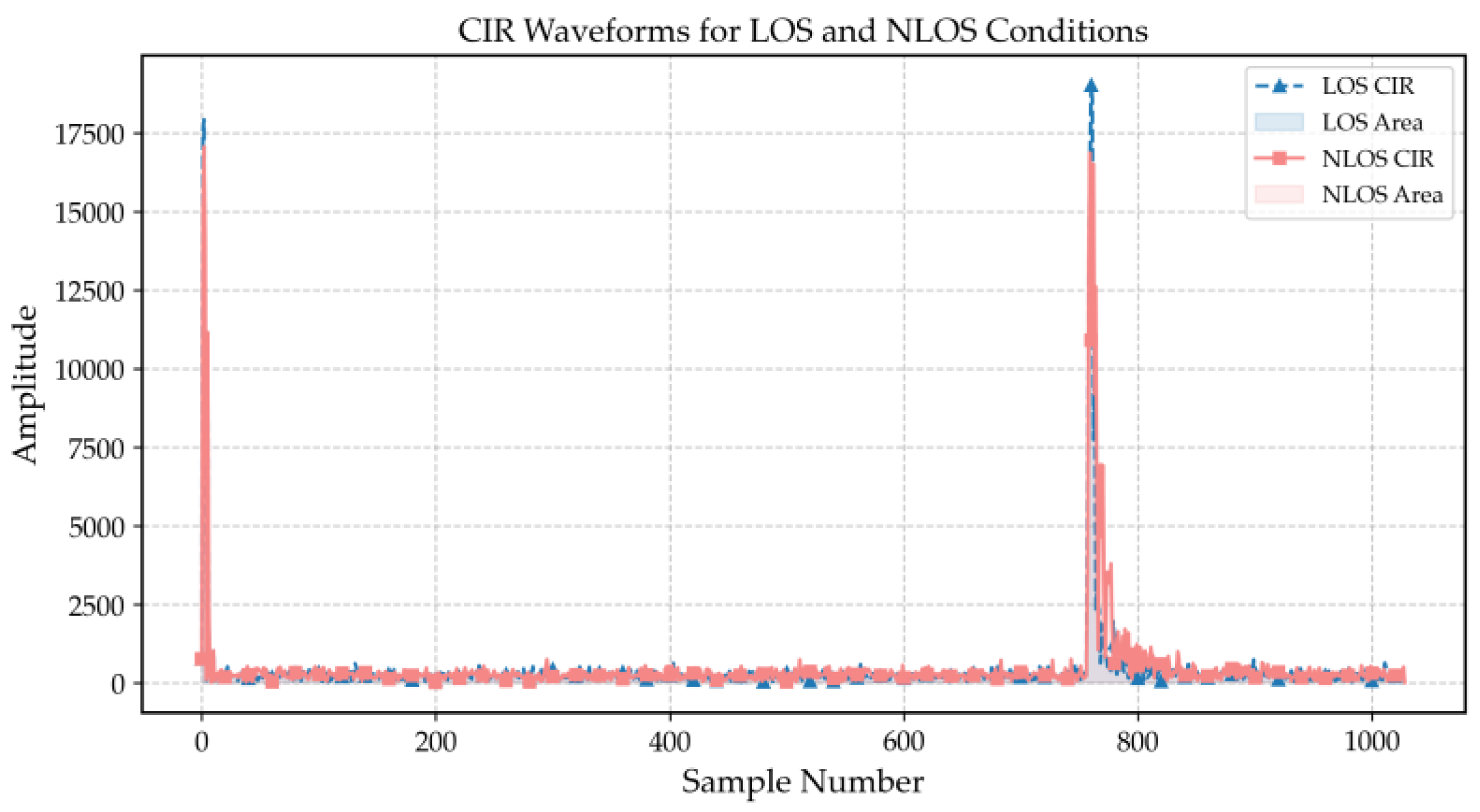
Figure 2.
Path amplitude diagrams in LOS and NLOS environments. (a) FP_AMP1. (b) FP_AMP2. (c) FP_AMP3.
Figure 2.
Path amplitude diagrams in LOS and NLOS environments. (a) FP_AMP1. (b) FP_AMP2. (c) FP_AMP3.
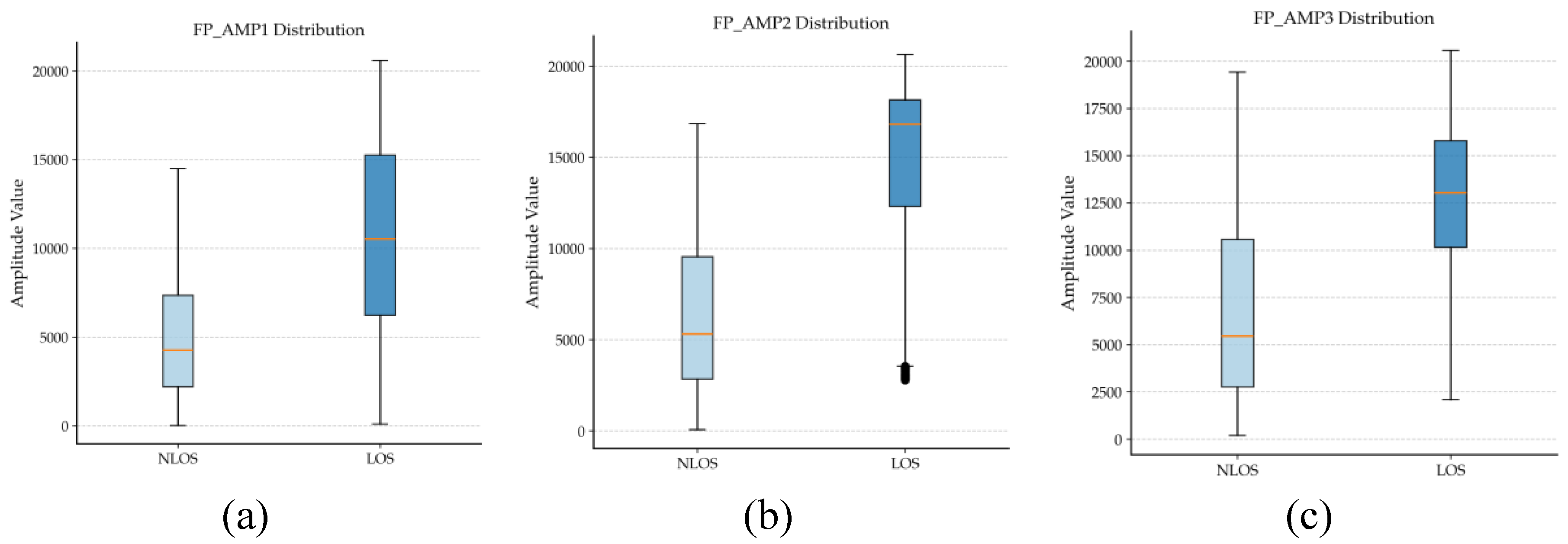
Figure 3.
Box plots of noise characteristics under NLOS and LOS conditions. (a) Maximum noise value. (b) Noise standard deviation.
Figure 3.
Box plots of noise characteristics under NLOS and LOS conditions. (a) Maximum noise value. (b) Noise standard deviation.
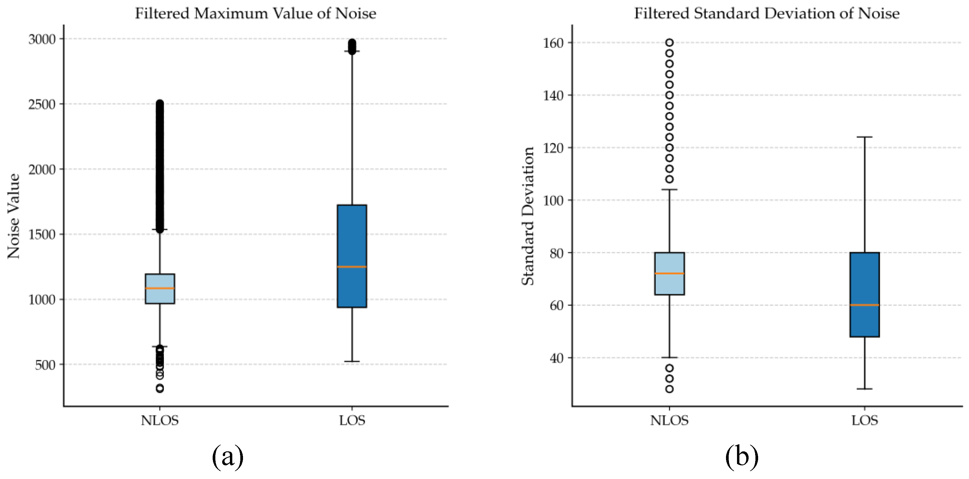
Figure 4.
Box plot of CIR power.
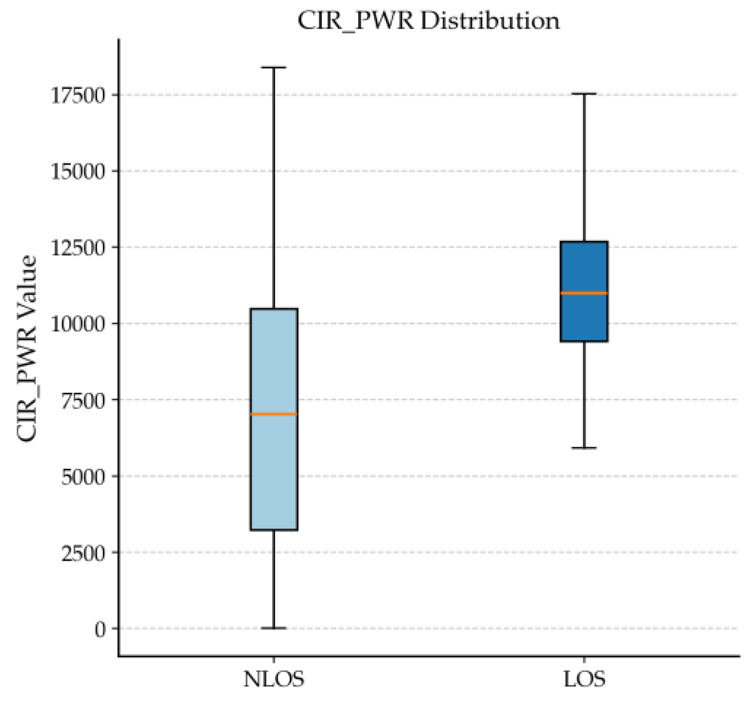
Figure 5.
Architecture of the BiLSTM.
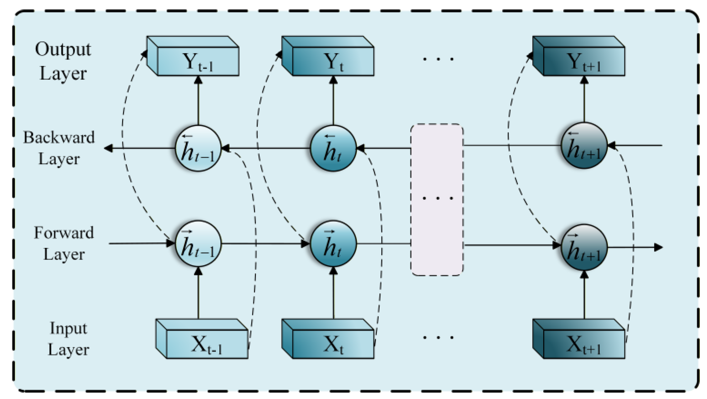
Figure 6.
Confusion Matrix Plots of Four Models. (a) BP. (b) MBP. (c) RF. (d) IPSO-MBP. (e) ISO-MBP.
Figure 6.
Confusion Matrix Plots of Four Models. (a) BP. (b) MBP. (c) RF. (d) IPSO-MBP. (e) ISO-MBP.
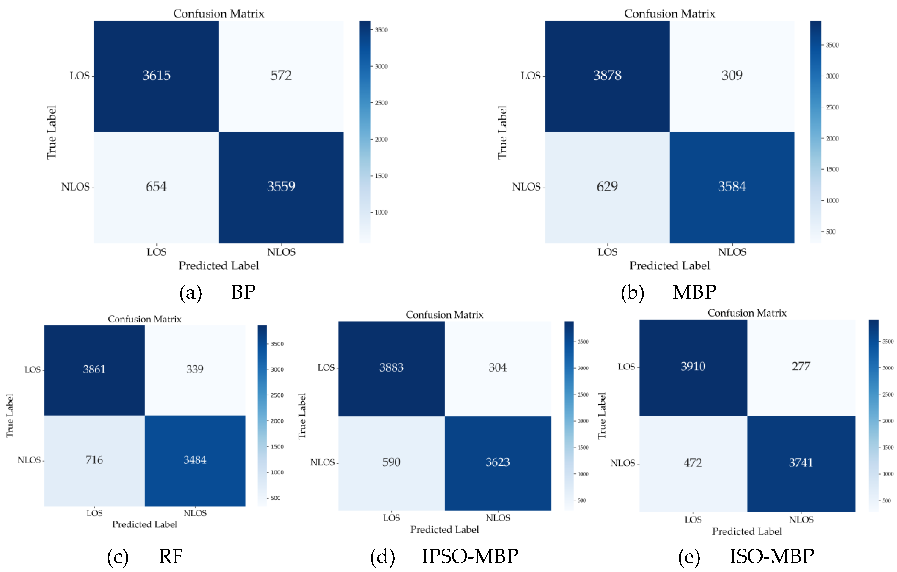
Figure 7.
Comparison of anchor-level RMSE under four environments. (a) Env 0. (b) Env1. (c) Env 2. (d) Env 3.
Figure 7.
Comparison of anchor-level RMSE under four environments. (a) Env 0. (b) Env1. (c) Env 2. (d) Env 3.
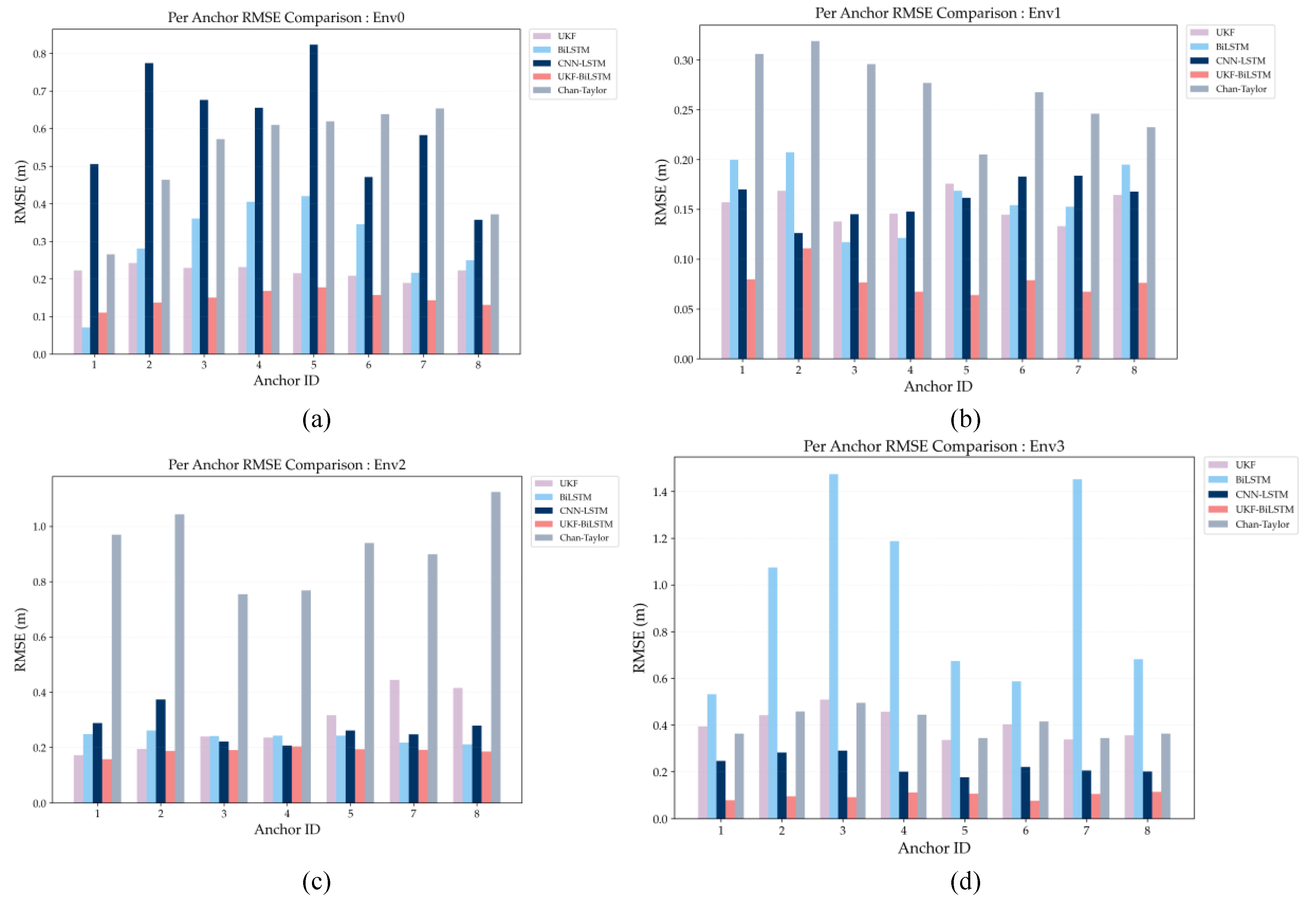
Figure 8.
Comparison of positioning error CDFs under four environments. (a) Env 0. (b) Env 1. (c) Env 2. (d) Env 3.
Figure 8.
Comparison of positioning error CDFs under four environments. (a) Env 0. (b) Env 1. (c) Env 2. (d) Env 3.
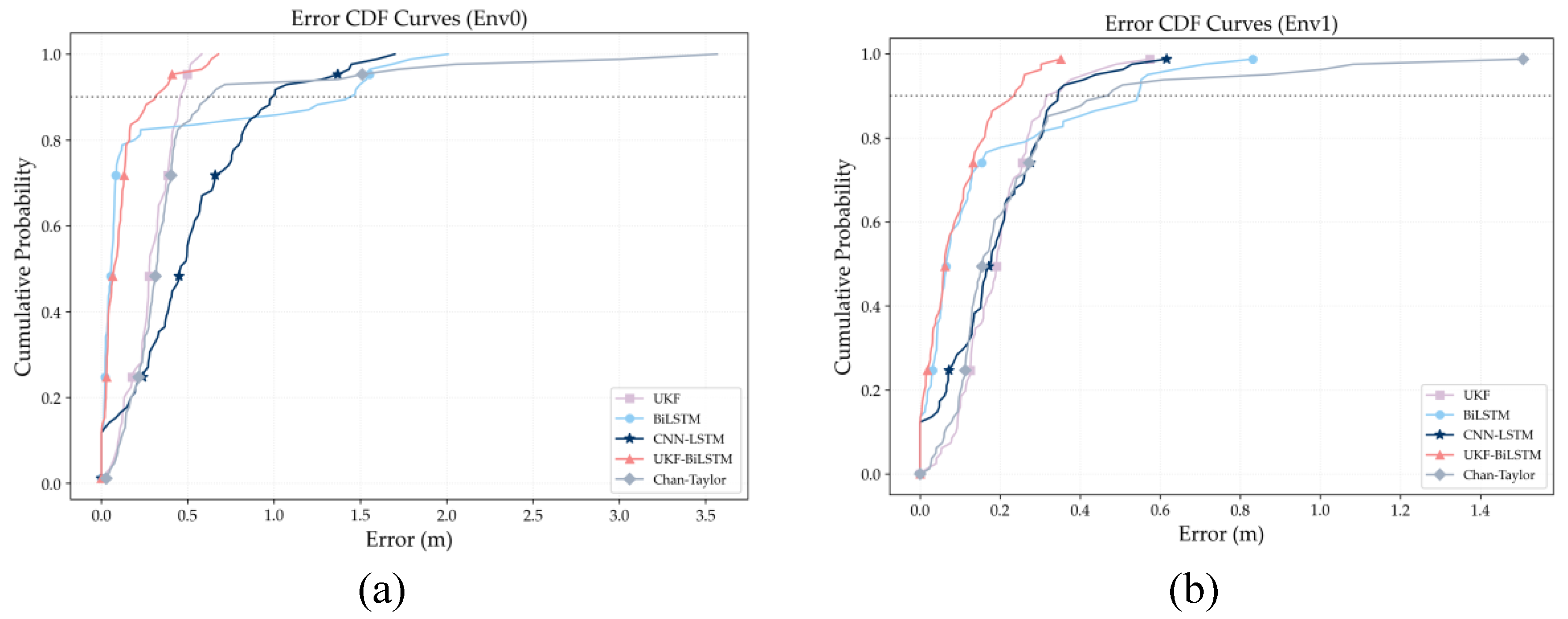
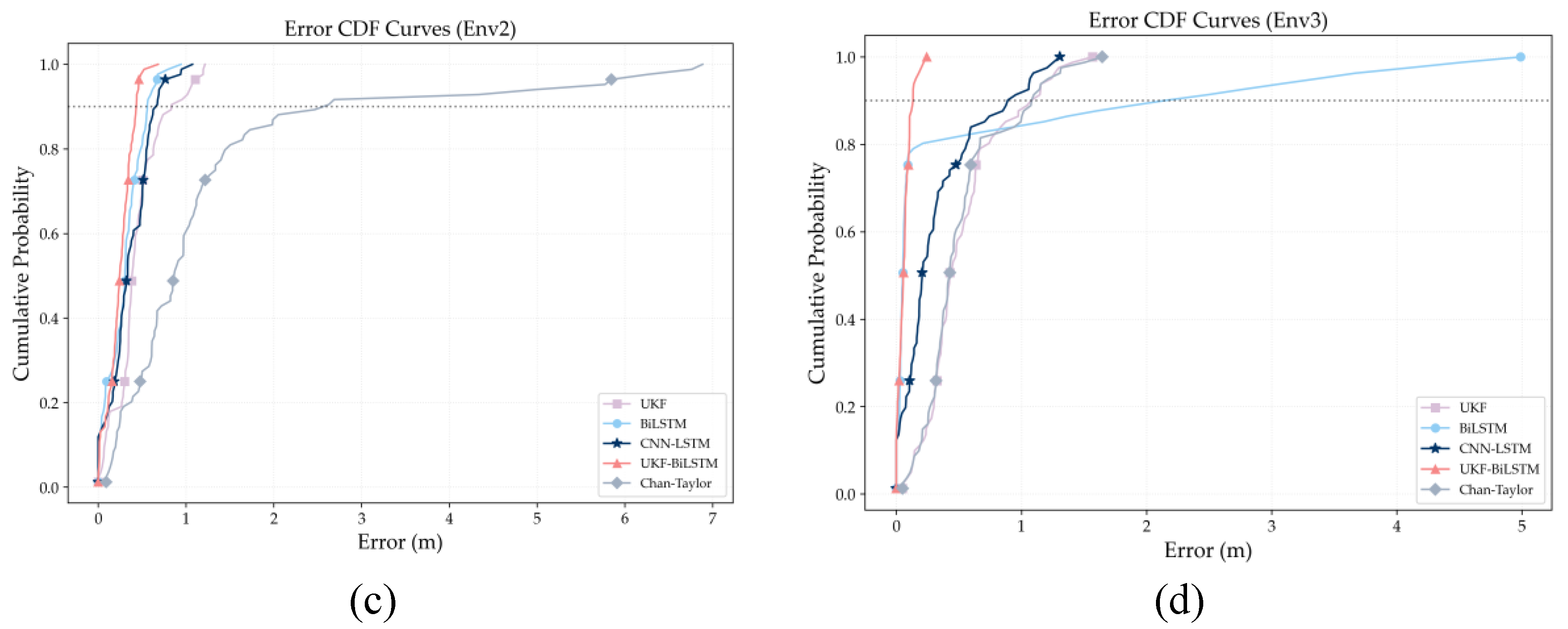
Figure 9.
Trajectories of UKF-BiLSTM under four environments. (a) Env 0. (b) Env 1. (c) Env 2. (d) Env 3.
Figure 9.
Trajectories of UKF-BiLSTM under four environments. (a) Env 0. (b) Env 1. (c) Env 2. (d) Env 3.
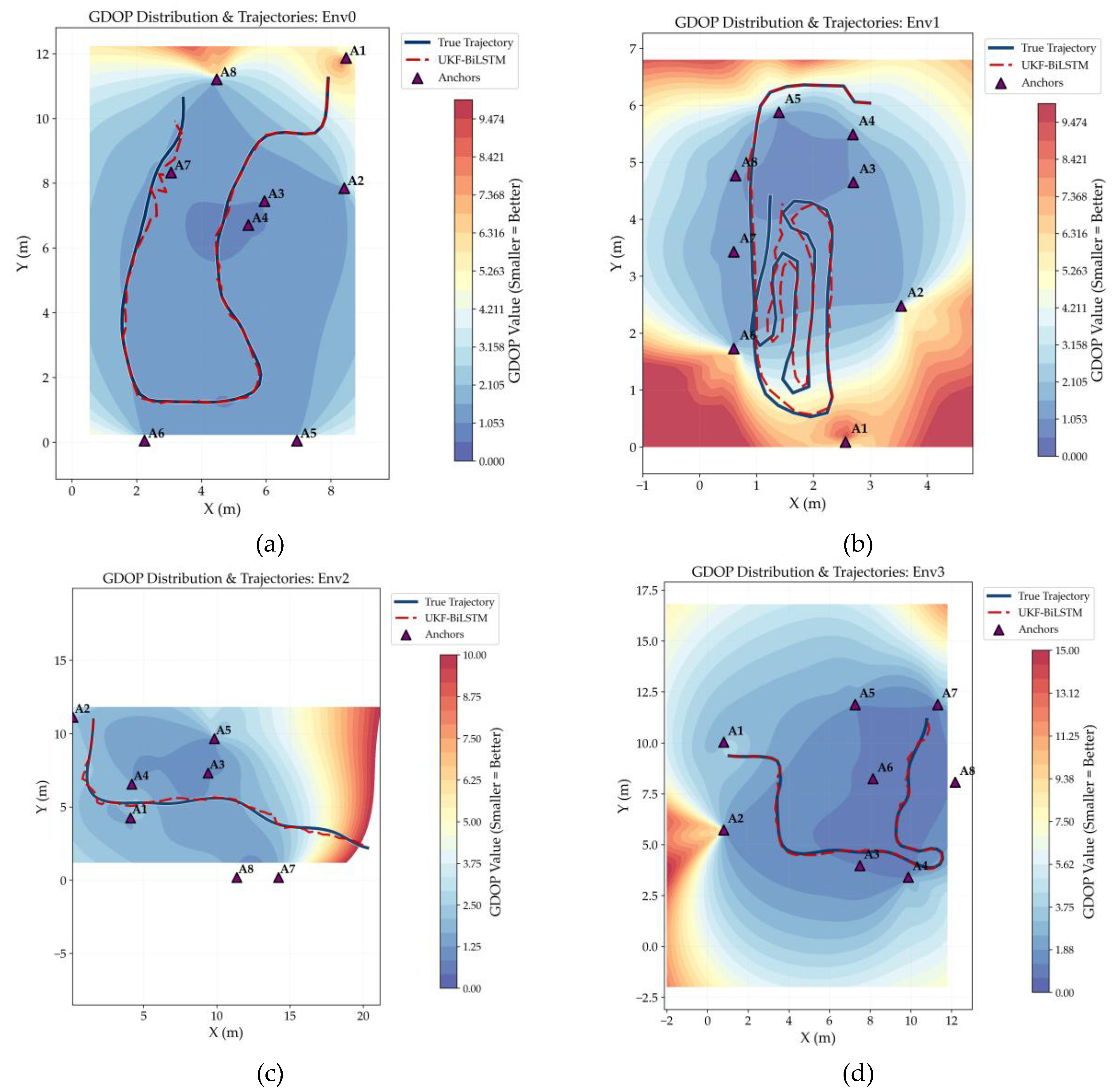

Table 1.
Overview of the NLOS error mitigation dataset.
| Env | Type | NLOS Conditions | Preprocessing |
|---|---|---|---|
| 0 | Large residential apartment 9.18 × 12.06 m brick exterior + plasterboard interior |
Few NLOS, only 5 outliers. |
Basic deviation compensation |
| 1 | Compact residential apartment 3.60 × 6.69 m concrete exterior + plaster interior |
Minimal NLOS, no abnormal values. |
Basic deviation compensation |
| 2 | Industrial workshop 21.96 × 11.85 m dense metal equipment |
High NLOS, strong multipath. |
Basic deviation compensation DBSCAN denoising (metal reflection outliers) antenna delay compensation |
| 3 | Office 15.37 × 11.50 m concrete exterior + plasterboard partitions |
Significant NLOS, 22 outliers. |
Basic deviation compensation DBSCAN denoising (partition NLOS outliers) antenna delay compensation |
Table 2.
Configuration of baseline models BP and MBP.
| Parameter Category | Parameter | BP Model | MBP Model |
|---|---|---|---|
| Network architecture | Input layer | 10 | 10 |
| Hidden layer 1 | 150 | 150 | |
| Hidden layer 2 | 75 | 75 | |
| Output layer | 2 | 2 | |
| Training configuration | Attention mechanism | None | MHSA(6 heads) |
| Optimizer | Adam | Adam | |
| Learning rate | 0.001 | 0.001 | |
| Training epochs | 200 | 200 |
Table 3.
Parameter settings of the hybrid optimization algorithms.
| Parameter Category | Parameter | IPSO-MBP Model | ISO-MBP Model |
|---|---|---|---|
| Basic configuration | Population size() | 10 | 10 |
| Maximum iterations () | 150 | 150 | |
| Parameter search range | |||
| Hybrid strategy | ICMIC chaotic map | ||
| DE scaling factor | |||
| DE crossover probability | |||
| Specific parameters |
Table 4.
Comparison of the performance of different algorithms.
| Model | Accuracy | Precision | Recall | F1-Score | Model Parameters(K) |
Training Time(s) | Inference Latency(ms) |
|---|---|---|---|---|---|---|---|
| BP | 85.40% | 86.15% | 84.48% | 85.31% | 13127 | 463 | 0.04 |
| MBP | 88.83% | 92.06% | 85.07% | 88.31% | 103727 | 669 | 0.16 |
| RF | 87.44% | 87.74% | 87.44% | 87.42% | 1324 | 55 | 24.41 |
| IPSO-MBP | 89.36% | 92.26% | 86.00% | 89.02% | 103727 | 1576 | 0.17 |
| ISO-MBP | 91.08% | 93.11% | 88.80% | 90.52% | 103727 | 1282 | 0.16 |
Table 5.
Unified model configuration parameters.
| Item | BiLSTM | CNN-LSTM | UKF-BiLSTM | |
|---|---|---|---|---|
| Input features | UWB ranging | -dim | -dim | -dim |
| UKF state | 5-dim | 5-dim | 5-dim | |
| Historical position | 2-dim | 2-dim | 2-dim | |
| Total feature dimension | +7 | +7 | +7 | |
| Training configurations |
Learning rate | 0.001 | 0.001 | 0.001 |
| Optimizer | Adam | Adam | Adam | |
| Training epochs | 100 | 100 | 100 | |
| Batch size | 32 | 32 | 32 | |
| Sequence length | 10 | 10 | 10 | |
| Hidden size | 64 | 128 | 64 | |
| Core architecture | Two-layer BiLSTM | CNN + three-layer LSTM | UKF–BiLSTM bidirectional mutual calibration |
|
Table 6.
Core parameters of BiLSTM and UKF.
| Model | Parameter Category | Parameter Name | Env0 | Env1 | Env2 | Env3 |
|---|---|---|---|---|---|---|
| BiLSTM | Network structure | Number of layers | 2 | 2 | 2 | 2 |
| Hidden layer size | 64 | 64 | 64 | 64 | ||
| Sequence length | 10 | 10 | 10 | 10 | ||
| Training config | Learning rate | 0.001 | 0.001 | 0.001 | 0.001 | |
| Batch size | 32 | 32 | 32 | 32 | ||
| Training epochs | 100 | 100 | 300 | 100 | ||
| UKF | Initial state | Initial velocity | 0.4m/s | 0.3m/s | 0.8m/s | 0.2m/s |
| Process noise | Velocity noise | 0.15 | 0.1 | 0.3 | 0.08 | |
| Angular velocity noise | 0.08 | 0.05 | 0.12 | 0.03 | ||
| Measurement noise | Measurement noise | 0.25 | 0.15 | 1.4 | 0.3 | |
| UKF params | Sigma params () | (0.1,2,-2) | (0.1,2,-2) | (0.01,2,0) | (0.1,2,-2) | |
| Dynamic calibration | Q/R rate | 0.5/0.3 | 0.4/0.2 | 0.6/0.3 | 0.6/0.4 |
Table 7.
Anchor-level RMSE in Env 0.
| Anchor | UKF/m | BiLSTM/m | Chan-Taylor/m | CNN-LSTM/m | UKF-BiLSTM/m |
|---|---|---|---|---|---|
| A1 | 0.2228 | 0.0712 | 0.2653 | 0.5054 | 0.1108 |
| A2 | 0.2423 | 0.2809 | 0.4636 | 0.7742 | 0.1368 |
| A3 | 0.2292 | 0.3605 | 0.5717 | 0.6759 | 0.1505 |
| A4 | 0.2318 | 0.4049 | 0.6099 | 0.6554 | 0.1681 |
| A5 | 0.2151 | 0.4202 | 0.6192 | 0.8231 | 0.1774 |
| A6 | 0.2088 | 0.3454 | 0.6387 | 0.4710 | 0.1572 |
| A7 | 0.1896 | 0.2163 | 0.6537 | 0.5826 | 0.1435 |
| A8 | 0.2228 | 0.2496 | 0.3718 | 0.3575 | 0.1308 |
Table 8.
Anchor-level RMSE in Env 1.
| Anchor | UKF/m | BiLSTM/m | Chan-Taylor/m | CNN-LSTM/m | UKF-BiLSTM/m |
|---|---|---|---|---|---|
| A1 | 0.1572 | 0.1999 | 0.3060 | 0.1700 | 0.0798 |
| A2 | 0.1686 | 0.2074 | 0.3190 | 0.1263 | 0.1110 |
| A3 | 0.1378 | 0.1173 | 0.2958 | 0.1452 | 0.0768 |
| A4 | 0.1458 | 0.1214 | 0.2769 | 0.1479 | 0.0675 |
| A5 | 0.1759 | 0.1688 | 0.2051 | 0.1617 | 0.0640 |
| A6 | 0.1449 | 0.1542 | 0.2677 | 0.1830 | 0.0789 |
| A7 | 0.1330 | 0.1528 | 0.2461 | 0.1838 | 0.0675 |
| A8 | 0.1645 | 0.1950 | 0.2326 | 0.1678 | 0.0762 |
Table 9.
Anchor-level RMSE in Env 2.
| Anchor | UKF/m | BiLSTM/m | Chan-Taylor/m | CNN-LSTM/m | UKF-BiLSTM/m |
|---|---|---|---|---|---|
| A1 | 0.1720 | 0.2483 | 0.9699 | 0.2879 | 0.1573 |
| A2 | 0.1943 | 0.2614 | 1.0433 | 0.3735 | 0.1874 |
| A3 | 0.2394 | 0.2415 | 0.7547 | 0.2213 | 0.1906 |
| A4 | 0.2359 | 0.2426 | 0.7684 | 0.2065 | 0.2032 |
| A5 | 0.3163 | 0.2430 | 0.9395 | 0.2608 | 0.1933 |
| A6 | None | None | None | None | None |
| A7 | 0.4442 | 0.2172 | 0.8993 | 0.2469 | 0.1910 |
| A8 | 0.4150 | 0.2113 | 1.1244 | 0.2792 | 0.1849 |
Table 10.
Anchor-level RMSE in Env 3.
| Anchor | UKF/m | BiLSTM/m | Chan-Taylor/m | CNN-LSTM/m | UKF-BiLSTM/m |
|---|---|---|---|---|---|
| A1 | 0.3942 | 0.5320 | 0.3629 | 0.2460 | 0.0795 |
| A2 | 0.4419 | 1.0746 | 0.4576 | 0.2825 | 0.0964 |
| A3 | 0.5085 | 1.4742 | 0.4954 | 0.2906 | 0.0924 |
| A4 | 0.4570 | 1.1876 | 0.4439 | 0.2007 | 0.1123 |
| A5 | 0.3361 | 0.6734 | 0.3446 | 0.1765 | 0.1070 |
| A6 | 0.4036 | 0.5870 | 0.4151 | 0.2202 | 0.0775 |
| A7 | 0.3378 | 1.4528 | 0.3445 | 0.2053 | 0.1068 |
| A8 | 0.3559 | 0.6817 | 0.3631 | 0.2010 | 0.1153 |
Disclaimer/Publisher’s Note: The statements, opinions and data contained in all publications are solely those of the individual author(s) and contributor(s) and not of MDPI and/or the editor(s). MDPI and/or the editor(s) disclaim responsibility for any injury to people or property resulting from any ideas, methods, instructions or products referred to in the content. |
© 2025 by the authors. Licensee MDPI, Basel, Switzerland. This article is an open access article distributed under the terms and conditions of the Creative Commons Attribution (CC BY) license (http://creativecommons.org/licenses/by/4.0/).
Copyright: This open access article is published under a Creative Commons CC BY 4.0 license, which permit the free download, distribution, and reuse, provided that the author and preprint are cited in any reuse.


