1. Introduction
Decision-making in multiagent systems often requires reconciling heterogeneous preferences to achieve collective outcomes that balance efficiency, fairness, and personalization. Lexicographic Preference Trees (LP-Trees) have emerged as a compact and intuitive representation of agent priorities, capturing structured decision rules in a way that is both expressive and computationally manageable. However, efficiently measuring similarity between such structures—particularly when they are incomplete or partial (PLPs)—remains a persistent challenge. Without robust similarity measures, coalition formation and preference aggregation risk being misaligned, limiting their effectiveness in complex markets where diverse stakeholders must coordinate.
To address this gap, we propose PLPSim, a new measure for quantifying similarity between PLP-Trees. PLPSim enables agents with comparable lexicographic preferences to be grouped into coalitions, thereby facilitating contract formation and collective decision-making. Building on this foundation, we design coalition formation algorithms that operationalize PLPSim, allowing diverse stakeholders to align their priorities through structured coalition mechanisms. Recognizing the importance of evaluation, we further introduce F@LeX, a novel metric tailored to lexicographic preferences, which provides a principled way to assess coalition quality and preference satisfaction. As for the need for PLP-tree dataset, we generate a synthetic dataset by presenting PLPGen algorithm. Together, PLPSim, ContractLex and PriceLex variants, and F@LeX form a methodological framework that advances preference-driven coalition formation in multiagent systems.
The relevance of this framework can be appreciated in light of prior research. Foundational studies in computational social choice have explored the representation and learning of lexicographic preferences [
1,
2], while more recent work has examined clustering and complexity aspects of partial LP-Trees [
3,
4]. Coalition formation and mechanism design have also been studied extensively in electronic commerce and group-buying contexts [
5], highlighting the importance of cost-sharing and preference alignment. In parallel, preference disaggregation and aggregation methods have been advanced in decision support systems [
6,
7], underscoring the need for rigorous similarity measures. Our study builds on these strands by introducing PLPSim as a dedicated similarity measure for PLPs and by proposing coalition algorithms that directly leverage this measure.
As an illustrative case study, we contextualize the framework within
hybrid renewable energy tariffs, a domain characterized by diverse consumer priorities, supplier strategies, and policy constraints. Prior studies have examined macro-level mechanisms such as feed-in-tariff policies [
8], adaptive strategy optimization using evolutionary game theory and reinforcement learning [
9], and risk-sharing support schemes to mitigate spot price volatility [
10]. Broader reviews of hybrid renewable energy systems optimization highlight the role of metaheuristic algorithms, simulation tools, and emerging technologies in improving efficiency and sustainability [
11,
12]. Additional research has applied game-theoretical methods to electricity markets [
13] and evolutionary game theory to complex systems optimization [
14]. While these studies emphasize system-level or policy-level design, our work focuses on
micro-level coalition mechanisms, where consumer PLP-Trees are aggregated and matched with supplier tariffs to improve personalization, efficiency, and fairness.
In summary, this study advances a methodological framework rather than prescribing domain-specific results. It contributes (i) PLPSim, a new similarity measure for complete and partial LP-Trees; (ii) coalition formation algorithms that leverage PLPSim to group agents with similar preferences; (iii) ContractLex and PriceLex, personalised coalition-based contracts and pricing strategies; (iv) PLPGen synthetic data generator; (v) F@LeX, a novel evaluation metric for lexicographic preferences; and (vi) an illustrative case study in hybrid renewable energy tariffs that demonstrates the practical utility of the framework. While electricity tariffs serve as the motivating example, the proposed approach generalizes to diverse multiagent systems, offering a versatile foundation for preference-driven coalition formation, adaptive policy design, and broader system optimization.
Organization of the article. Related works are reviewed in
Section 2; the method is proposed in
Section 3; the experimental results are illustrated in
Section 4; and the article is concluded with future avenues in
Section 5.
3. Methodological Framework
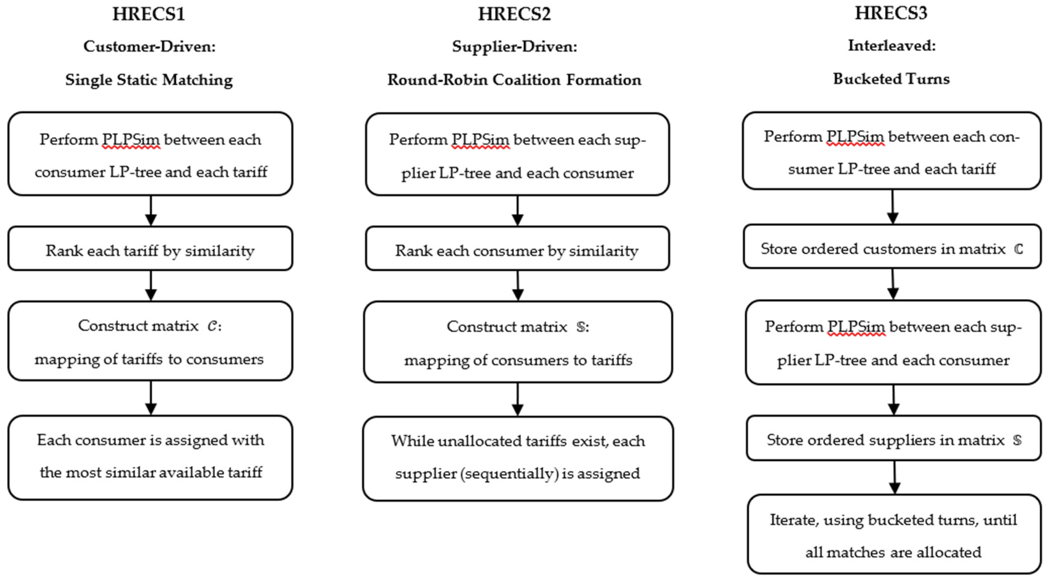
This section presents main parts of our methodological contributions: a similarity measure for PLP-Trees (PLPSim), coalition formation algorithms (HRECS1, HRECS2, HRECS3) that exploit preference similarity, and lexicographic contracts and pricing strategies (CLF, CFB, CFW, CFA, CFP). Together, these components form a coherent framework for modeling, forming, and evaluating coalitions in multiagent environments where preferences are expressed lexicographically. We also present PLPGen method for generating lexicographic preferences synthetic dataset (Appendix). Moreover, we propose F@LeX, a novel evaluation metric designed to capture the quality of coalition outcomes in lexicographic preference settings.
To illustrate the allocation challenge that motivates our framework, consider the problem of assigning hybrid renewable electricity tariffs in a future competitive energy market, in which consumers and suppliers express their priorities as lexicographic preferences: price acts as a hard constraint, while attributes such as energy type, reliability, and contract length serve as negotiable dimensions. Consumers seek affordable tariffs, suppliers aim to maximize profit, and group discounts create incentives for coalition formation. Moreover, each consumer may value these attributes differently — for example, one may prioritize low cost, while another emphasizes environmental sustainability. Grouping the most similar consumers with the same consumption pattern and fair payments maximize the satisfaction of each consumer in the coalition. This example highlights the need for robust similarity measures, coalition algorithms, and evaluation metrics for such kind of preferences, which we develop in the following subsections.
We first build formal foundations on the PLP-Tree structures through a case study in hybrid renewable energy tariffs in
Section 3.1.
Section 3.2 introduces PLPSim;
Section 3.3 presents coalition formation algorithms;
Section 3.4 describes lexicographic contracts and pricing strategies; and
Section 3.5 introduces the evaluation metrics for PLP-trees;
Section 3.6 presents computational representation for implementing PLP-trees.
3.1. Lexicographic Preference Tree Solution Rank
To compute solution ranks in lexicographic preference trees (LP-trees), we traverse the tree in pre-order from root to leaf.
Figure 1 illustrates the traversal process used to enumerate solutions, which underpins the ranking definitions introduced below. Beginning with the left branch, all possible combinations of attribute values (e.g., D: contract duration, E: energy type, S: ancillary services) are enumerated, each combination representing a solution. For simplicity, assume attributes are binary (e.g., d and d′ for D). so each node has at most two children.
We assume suppliers typically express tariffs using complete lexicographic preferences (CLP), since they know all attributes and values. Consumers, however, may provide either complete or partial lexicographic preferences (PLP), due to limited information or an inability to distinguish between certain attributes or values.
We extend the standard LP-tree formalism by introducing the notion of partial solutions. If value substitution is not performed on all attributes of the problem, ordering these values is an incomplete or partial solution. This concept is critical because coalition algorithms must operate even when consumer preferences are incomplete. To compare this with the preferences of the supplier, we introduce shared parts between their complete and partial LP-trees, defined as follows.
Definition 2 (Shared partial solution). Let the problem has attributes, and let and denote a complete and a partial LP-tree, respectively. If at least one branch of contains fewer than attributes, then for and , is a shared partial solution iff and .
Unlike measures in comparing CP-nets [
16] and as a prerequisite for PLPSim, we distinguish between solutions by considering their position in the list of preferences, so that the best solution receives rank
n (equal to the number of leaves, i.e., the total number of solutions), while the worst solution receives rank 1.
Definition 3 (Solution rank in lexicographic preferences). Solutions in a lexicographic preferences
(LP-tree) are ranked according to Eq. (1), in which, solution
is indexed according to its position in the linear preference order.
The idea behind solution ranking is to translate the qualitative order of preferences into a quantitative scale that can be compared across LP-trees of different sizes. Without normalization, a tree with 8 leaves and a tree with 20 leaves would produce ranks on very different scales, making comparisons inconsistent. Normalization rescales all ranks to the interval [0, 1], ensuring that ``best’’ and ``worst’’ solutions are always comparable regardless of tree size (Eq. 2). Since a normalized value of 0 eliminates the worst solution, a small positive constant λ (e.g., 0.1) is added to shift the range; hence. every solution retains a positive score, with the best solution close to 1 and the worst solution slightly above zero (Eq. 1). For example, and .
Having established how solutions in lexicographic preference trees can be ranked and normalized, we now turn to the problem of measuring similarity between different lexicographic preferences. This motivates the introduction of PLPSim, our proposed similarity measure that extends beyond existing approaches such as PLPDis.
3.2. Lexicographic Preference Similarity Measure: PLPSim
Lexicographic: Preference Trees (LP-Trees) capture agent priorities in a compact form, but comparing complete or partial structures (PLPs) requires a principled similarity measure. We build on PLP-Trees to introduce PLPSim, a similarity measure that extends beyond prior work by handling both complete and partial trees, while integrating structural and semantic components, enabling robust similarity assessment even when agents specify incomplete lexicographic orders.
The only existing method, PLPDis, for comparing two complete or partial lexicographic preference trees
, and
computes their distance by applying the partial Kendall distance [
3]. It forgets the absence of attributes in partial trees (
Table 1); e.g., it computes the distance from
to
as its horizontal mirror
to
. For addressing this issue, we introduced the rank of solutions (Definition 3) and by adapting, extending, and improving CPSim (in CP-nets context) [
16] to lexicographic preferences, present PLPSim method. PLPSim distinguishes between tree branches and the importance and preference of solutions of the LP-tree in computing the similarity of complete and partial preferences (PLP).
Let each agent’s preferences be represented as a Partial Lexicographic Preference Tree (PLP-Tree), where each node corresponds to an attribute and edges encode lexicographic priority ordering. For the two
and
PLP-trees represented by graphs
and
, we calculate PLPSim of
to
through Eq. (3), the average of three fractions, where,
,
,
,
,
and
are the count of shared variables between
and
, the count of shared edges between
and
, the count of variables in
, the count of edges in
, the sum of the rank product of the shared solutions between the two
and
trees, and the sum of the square roots of the ranks of the
solutions;
and
[
20].
PLPSim establishes a total binary order relationship on lexicographic preferences, as follows.
Theorem 1 (PLPSim Total order). The similarity of lexicographic preferences with lexicographic preferences satisfies asymmetric, reflective, and transitive properties:
That is, similarity measurement between lexicographic preference structures is asymmetric. This arises because attributes or values in the domain may not be shared across two comparisons. In one direction, one preference structure may be a subset of the other, while in the reverse direction, the inclusion does not hold. Consequently, it cannot be assumed that if structure is similar to structure to a certain degree, then must necessarily be similar to with the same degree. This asymmetry motivates the following theorem.
Theorem 2 (Asymmetric property of PLPSim similarity). Let
denote the similarity measure between two PLP-trees
and
, as defined in Equation (3). For both complete and partial LP-trees,
exhibits an antisymmetric property across all four compound cases, UI–UP, CI–UP, UI–CP, and CI–CP. Formally,
whenever the attribute sets or value domains of
and
are not identical, or when one tree is a subset of the other but not vice versa. Since the class of UP is a subset of FP, this important antisymmetric property extends to all six classes of lexicographic preferences described in
Section 2.2.
Corollary 1 (Practical implication of asymmetry). PLPSim similarity scores are inherently asymmetric and cannot be assumed equal in both directions.
This asymmetry highlights a fundamental challenge in coalition stability. A coalition that appears favorable when evaluated from the consumer’s perspective may not be equally favorable from the supplier’s perspective. As a result, coalition agreements must be negotiated with awareness of this imbalance, ensuring that both parties’ evaluations are considered. Ignoring asymmetry could lead to unstable coalitions, where one side perceives high similarity and alignment while the other side perceives low similarity, ultimately risking dissolution of the coalition.
Remark (Novelty compared to symmetric measures). Unlike symmetric measures such as CPSim [
16], which assume bidirectional equality of similarity scores between two graphical structures, PLPSim explicitly captures
directional asymmetry. This distinction is crucial: symmetric measures may overstate alignment between consumer and supplier preferences, while PLPSim reveals the nuanced differences that arise when one preference structure is a subset of another. This property underscores the methodological novelty of PLPSim and its relevance for coalition formation in heterogeneous preference environments, where consumer-to-supplier and supplier-to-consumer evaluations may diverge.
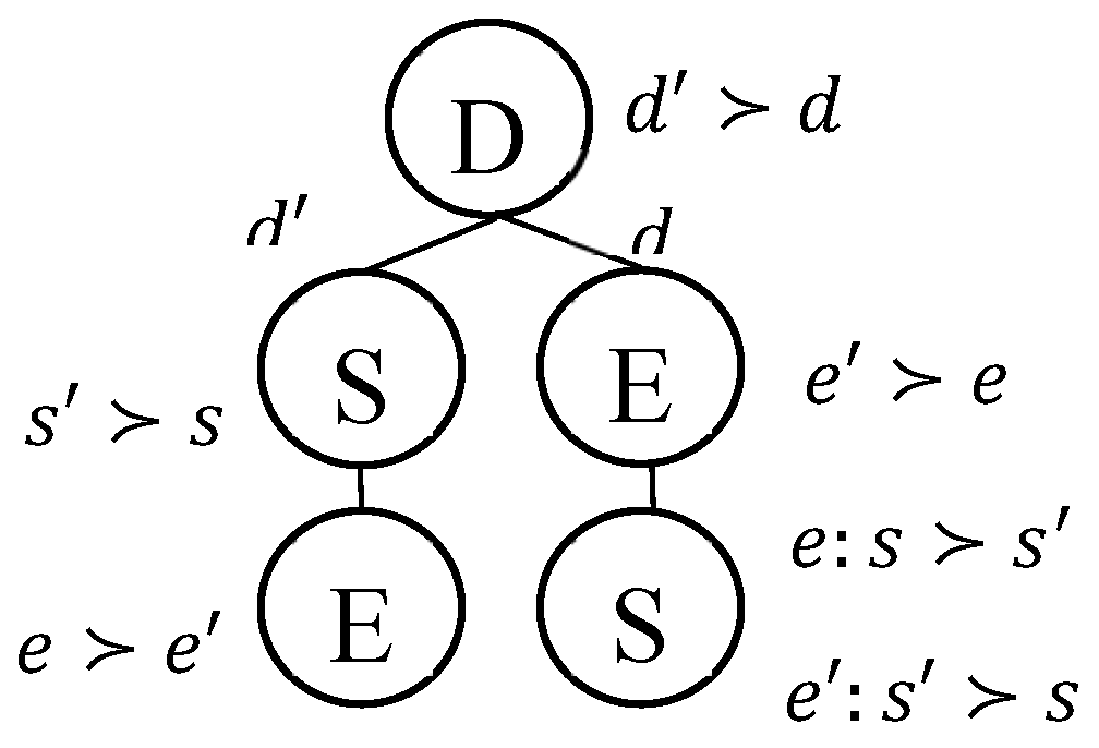
Figure 2, illustrating structural overlap of attribute orderings and semantic overlap of preference values, depicts a supplier’s complete tariff tree (2a) and two partial LP-trees (2b and 2c) representing two consumer’s partial preference structure, where the order of their solutions is opposite. In considering the scores of solutions of LP-trees in
Figure 2,
Table 1 highlights the antisymmetric property of PLPSim, and compares
PLPSim similarity measurement with CPSim, which ignores the directional similarity [
16] and PLPDis that suffers from forgetting some information in traversing partial trees [
3], along with LPDis, which does not work well in partial LP-trees [
35].
PLPSim measure forms the foundation for coalition formation, as it allows agents with comparable preferences to be grouped effectively.
Section 4.1 provides a step-by-step calculation of the PLPSim similarity score between a consumer’s preference tree and a supplier’s tariff tree, illustrating this asymmetric behavior in practice.
3.3. Coalition Formation Algorithms
Building on PLPSim directional similarity, we present HRECS coalition formation methods by assigning the most similar tariff to each consumer. Coalition formation proceeds in two stages: group agents into preference-aligned clusters and design a contract. We present three coalition systems: consumer-centric
HRECS1, supplier-centric
HRECS2, and market-driven
HRECS3, each representing different strategies for balancing coalition size and preference similarity. These systems integrate PLPSim into the coalition selection process, ensuring that agents with high similarity scores are aggregated. Coalition agreements are operationalized through
lexicographic contracts. Each contract specifies rules for tariff allocation and satisfaction balancing (
Section 3.4).
Conceptual diagrams of HRECS1, HRECS2, and HRECS3 in Figure 3 visually clarify the differences in how each algorithm performs matching. To establish a systematic foundation, we first formulate the coalition formation problem and present the general approach underlying the HRECS, before proceeding to the detailed formulations of its three variants in
Section 3.3.1,
Section 3.3.2 and
Section 3.3.3.
Figure 2.
Conceptual visualization: comparison of assigning each tariff to a group of similar consumers by using HRECS1, HRECS2, and HRECS3 matching.
Figure 2.
Conceptual visualization: comparison of assigning each tariff to a group of similar consumers by using HRECS1, HRECS2, and HRECS3 matching.
The sets of suppliers and consumers of hybrid renewable energy systems (HRECS) consist of and , respectively. Assume that each supplier offers a tariff where, , , , and are the LP-tree, the lowest acceptable price, the least count of people required for forming a coalition over the tariff, and ID of , respectively. Each consumer can bid his energy requirement , where , , and are the LP-tree, the highest acceptable price, and ID of , respectively. In this setup, consumer can buy tariffs that . For the supplier , the bids is considered if , that is, and . In these sets , the similarity of LP-trees is compared with LP-tree; then, s that satisfy the condition are sorted in descending order of their trees similarity with , so that , where or . Matrix forms ordered lists of tariffs similar to consumers’ preferences, and matrix forms ordered lists of consumers similar to tariffs’ preferences. Because the symmetry of the similarity function is not needed, the matrix is not necessarily obtainable from , and vice versa. If in and , suppliers are arranged in ascending order, and consumers in descending, , based on the bid price, from matrix and , ordered matrix and are yield, which is arranged in the order of price decrease and price increase, respectively, and contains ordered lists of tariffs similar to consumer preferences and ordered lists of consumer preferences similar to tariffs.
3.3.1. HRECS 1: Consumer’s PLP-Driven Coalition Formation
Building on the general formulation of HRECS, we now present the first algorithmic variant, which serves as the foundation. Having a matrix
from the ordered lists of tariffs in
for each consumer
, the most similar tariff is allocated to each consumer according to Algorithm 1 (line 5). The order in which consumers' requests are processed does not affect the outcome, and each consumer receives the only tariff that is the most similar to their preferences,
without any restrictions. According to this allocation, by inverting
, for each tariff
Group
is formed from the most similar consumers possible.
| Algorithm 1. HRECS1 |
1: Input:
2: Output:
3: Begin
4: for each do
5:
6: // i.e., add to ~ add to
7: end for
8: return
9: End |
3.3.2. HRECS 2: Supplier’s LP-Driven Coalition Formation
Unlike the HRECS1 approach, this approach allocates tariffs at the request of suppliers. Because each consumer receives its electricity from only one energy supplier through the tariff, concerning the sharing and conflict of the supplier list regarding the most similar consumer preferences, the order of consideration of the suppliers in the result of the consumer allocation affects the suppliers. This approach arranges the tariffs in the sense that the one with the lowest price has the highest priority; consequently, the ordered matrix containing ordered lists of tariff preferences similar to consumers is applied. This approach prevents suppliers from being ranked lower than consumers with similar preferences, Round Rubin shifts are applied in a cyclic manner.
According to Algorithm 2,
- (1)
by starting from the beginning of matrix , while a tariff exists where , the most similar consumer in the similarity list with the tariff is allocated to this tariff (line 6).
- (2)
Then, preference of the consumer is removed from the list of all tariffs in , (i.e. to (line 8).
- (3)
In the end, Step (1) continues with a cyclic turn of tariff (or If ).
Thus, for each tariff
, group
consists of the most similar possible consumers.
| Algorithm 2. HRECS2 |
1: Input:
2: Output:
3: Begin
4: while do
5: foreach do
6: // i.e., add to
7: foreach do
8: // i.e., delete from
9: end for
10: end for
11: end while
12: return 13: End
|
3.3.3. HRECS 3: Consumer’s PLP-Supplier’s LP-Driven Coalition Formation
The third approach focuses on both sides of the market, a combination of HRECS1 and HRECS2, with the difference that the order and turn is applied to consumers' demands, as well (i.e., matrix
and
). But for the turn to occur among the consumers and the suppliers and to establish a balance in handling the two sides of the market, a relative turn is applied inside. In this manner, after several sequential hearings on one side, it is the turn of the sequential hearings on the other side (
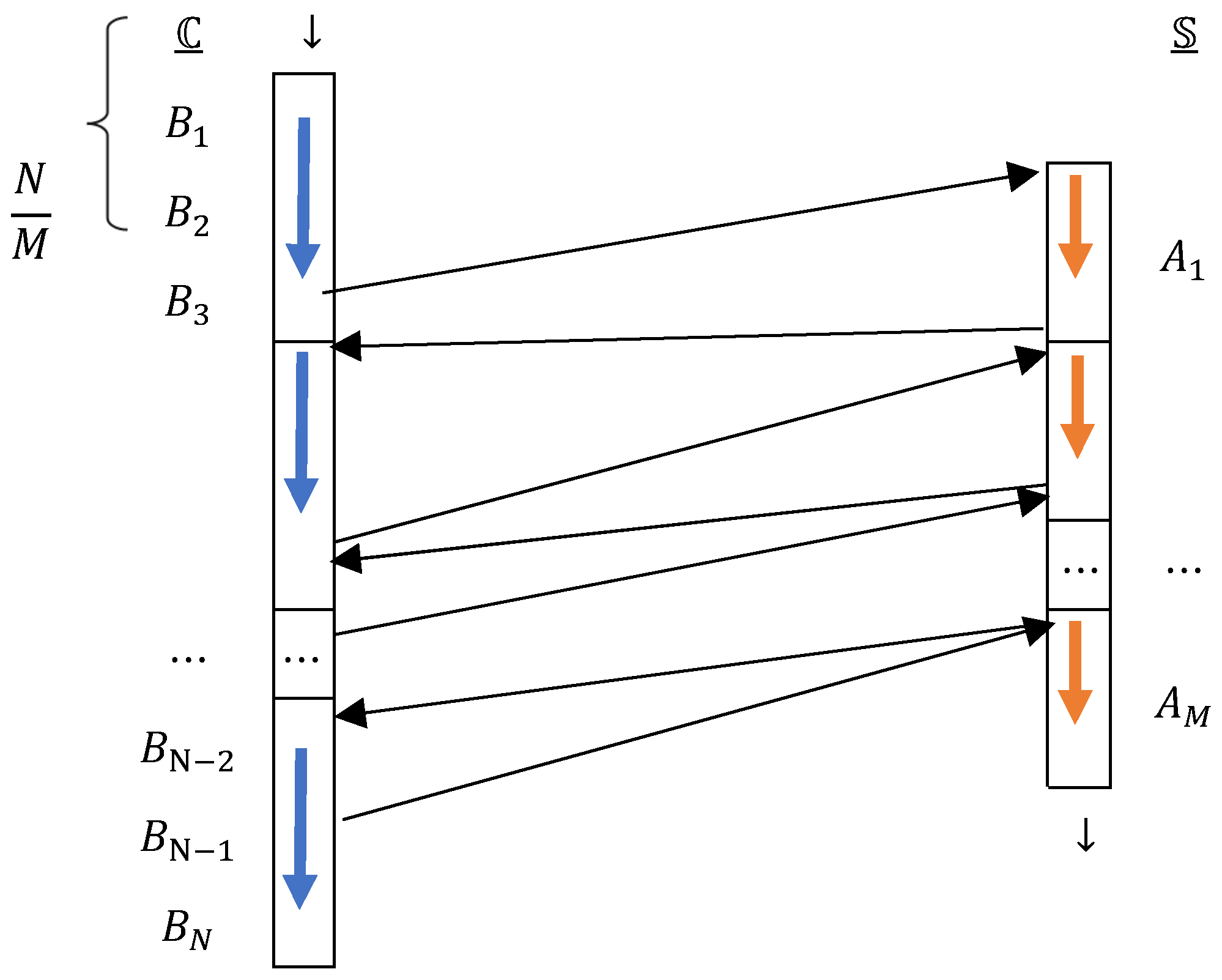
Figure 4). More expensive tariffs and cheaper demands are considered with a delay. All allocations are made at the end of the last matrix and without the need to rotate the turn to the beginning.
According to Algorithm 3, with the priority of starting the first consideration from or , this turn is not alternating; it switches between buckets of suppliers (length ) and buckets of consumers (length ): If , the length of the bucket is considered equal on both sides, for simplicity, is considered. Although the shorter the bucket length, the better the balance in giving priority to both sides and the count of changes of alternatives, the execution time increases; If , the length of the buckets is considered, , for simplicity, . If , the length of the buckets is considered, for simplicity, .
Beginning with the matrix and the two counters and , as long as there is a tariff where or a where ,
- (1)
for of consumers , the most similar tariff is assigned to each consumer; that is, demand of consumer is recorded in group for the tariff
(line 14),
- (2)
and the demand of this consumer is removed from the list of all tariffs in , (i.e. to ) (line 16),
- (3)
The pointer at the consumers’ side is incremented by 1 bucket (line 18),
- (4)
For the count of suppliers , the most similar consumer in the list of similarities to the tariff is placed for this tariff, respectively; that is, demand of consumer is recorded in group for the tariff (line 22),
- (5)
The preference line of this consumer is removed from (line 23),
- (6)
Preference of this consumer is removed from the list of all tariffs in , (i.e. to ) (line 25).
- (7)
The supplier pointer increases by one bucket (line 27);
- (8)
Step (1) continues.
Group
is formed of the most similar consumers possible to the tariffs of each supplier, by this interleaving turns among the preferences of consumers and suppliers.
| Algorithm 3. HRECS3 |
1: Input: ,
2: Output:
3: Begin
4:
5: if then
6:
7: elseif then
8:
9: endif
10:
11: while or do // i.e., or
12: foreach
13:
14:
15: foreach
16: // i.e., delete from
17 endfor
18:
19: endfor // and switches to the other matrix
20: foreach
21:
22:
23: // i.e., delete from
24: foreach
25 // i.e., delete from
26: endfor
27:
28: endfor // and switches to the other matrix
29: endwhile
30: return
31: End
|
3.4. Tariff Contracts
Contracts are applied after coalition formation to determine allocation outcomes. Because the prices of the proposed tariff may differ from the individual consumer preferences, the tariff implementation protocol must be specified after determining either the tariff for each consumer (Algorithm 1) or the set of consumers assigned to each tariff (Algorithms 2 and 3). Contracts may be defined as either fixed or variable agreements.
In this study, we introduce the concept of
lexicographic contract (ContractLex) and
lexicographic price (PriceLex), which reflects the changing and
dynamic nature of the hybrid renewable energy supply,
Section 3.4.1. This section describes how each consumer is assigned to a tariff based on their lexicographic preference tree. The contract details are embedded in the preference tree and offered to all consumers of that tariff. This setup is dynamic because the lexicographic contract is explicitly tied to the changing nature of the hybrid renewable energy supply. The consumer–supplier assignment can adapt as preferences or supply conditions shift, highlighting the flexibility required in hybrid renewable energy systems.
For fixed contracts–that embody
static coalition agreements once established—four implementation protocols are presented in
Section 3.4.2. Moreover, if a coalition is formed around a given tariff (i.e., the quorum of the minimum required consumers is met), the corresponding group discount is applied to the final tariff contract price. That is, once a coalition is formed and the quorum of consumers is met, the group discount applies, but the contract itself is static — it does not adapt to changes in supply or preferences. Hence, this setup is static, since the protocols lock in the contract terms once agreed, ensuring stability and predictability in coalition outcomes.
3.4.1. Lexicographic Contract: Dynamic Hybrid Renewable Energy Tariff
This section introduces the lexicographic contract of hybrid renewable energy tariffs, which reflects the inherently dynamic nature of both supply conditions and consumer preferences. Unlike fixed agreements, these contracts evolve as preference trees capture changing priorities and resource availability, thereby enabling coalitions to adapt in real time. This formulation highlights the flexibility required in hybrid renewable energy systems, where tariff structures and consumer assignments cannot remain static but must respond to ongoing variations in demand and supply.
Here, determines the appropriate tariff for each consumer. For each tariff, a group of consumers is assigned; that is, the preference tree of the same tariff states the contract details between the supplier of this tariff and these consumers, and this tree is offered to all. This tree contains many branches and conditions that well express the nature and variable nature of the hybrid renewable energy supply on the values of its attributes. Consumers subject to this lexicographic contract accept the risk that by paying the amount, they receive electrical energy with attributes that range over the values expressed by the solutions of this tariff. Suppliers subject to the same lexicographic contract accept the risk that consumer satisfaction may not be provided, and the tariff contract may be terminated before its expiration date. This type of contract fully reflects the market risks of this energy. Group discount is a way to cover this quality change and increase consumer satisfaction and retention under this contract, Definitions 4 and 5. The price of this contract can also be volatile, according to Proposition 1.
Definition 4 (ContractLex: Lexicographic Contract of hybrid renewable energy). The lexicographic contract of the hybrid renewable energy is the same for all consumers in the group so that its details are tailored by the lexicographic preferences of the tariff , and its price is a function of the lexicographic price function .
Definition 5 (PriceLexFixed: The fixed minimum price of the lexicographic contract of hybrid renewable energy). With the lexicographic contract
consumers and suppliers accept all terms and the fixed price, and the price determined for this contract includes all fluctuations in the range of all solutions of this tariff. This price is based on
, the highest price possible by all consumers
in group
of the tariff:
The minimum bid price in this group is the highest price that everyone in the group can pay; therefore, the final price of the contract is , where , indicating that the group has reached the quorum , all consumers in this coalition group on this energy tariff receive the same percent discount (e.g., =10%).
Proposition 1 (PriceLex: Lexicographic Price of hybrid renewable energy). If the range of values of the attributes of the lexicographic preferences is uniform and the direction is the same for all consumers and suppliers, the price of the energy supplied/received according to the changes in the solution provided in the contract becomes , where and corresponds to equations (2) and (4). The distance between this price and the minimum price of this tariff is the variable price fluctuation interval of the lexicographic contract of hybrid renewable energy, indicating that the worst solution of this tariff is with the price and the most valuable solution is at the price . In principle, the same direction means that the order of values is the same among all; both consumers and suppliers consider "solarwindgeothermal" as the energy type. Therefore, the best solution is considered the best solution for both.
3.4.2. Fixed Hybrid Renewable Energy Tariff Contract
This section presents the fixed contract protocols of hybrid renewable energy tariffs. A fixed contract represents only one solution from the range of fluctuations of the attributes of this type of energy and at a specific price of this solution; that is, although this energy is inherently prone to price fluctuations subject to contract, consumers and suppliers under a fixed contract agree that the solution is expected and a fixed price is set for it. Four types of fixed non-lexicographic contracts are offered to groups of consumers identified for Lexicographic Tariff as follows:
Definition 6 (ContractFixed: Best - CFB). In the contract , the best solution (i.e., the most left solution) of the LP-tree of the tariff is set for all consumers in . The price of this contract is obtained through the Equation .
Definition 7 (ContractFixed: Worst - CFW). In the contract , the worst solution (i.e., the most right solution) of the LP-tree of the tariff is set for all consumers in . The price of this contract follows from the Equation .
Definition 8 (ContractFixed: Average - CFA). In the contract , the middle solution in the LP-tree of tariff (i.e., with a for the supplier) is set for all consumers in . The price of this contract is obtained through the Equation .
Definition 9 (ContractFixed: Personalized - CFP). For each consumer
in
a specific contract
is concluded according to Algorithm 4. The value
for each solution,
is specified for
and assigned to
. If an
is not obtained from the LP-tree
,
, the solution
, with the highest value for
, is determined as a contract for this consumer
. The fixed price of the contract is set between the average prices
and
. If the count of consumers of this tariff
, reach the quorum of
, the contract price for each consumer
in this group is equal to nine-tenths (90 percent) of the specific price set for him, making,
.
| Algorithm 4. CFP |
1: Input:
2: Output:
3: Begin
4: foreach in do
5: foreach in do
6:
7: )
8:
9: endfor
10: endfor
11: return
12: End
|
3.5. Metrics
To assess the functionality of PLPSim between PLP-trees as well as the effectiveness of the proposed coalition formation strategies and contract mechanisms, we introduce a set of evaluation metrics that capture both performance and fairness dimensions.
We evaluate the quality of the coalition outcomes through the Davies-Bouldin dispersion index [
22], where the less DB, the better (Definition 10), and Normal Discounted Cumulative Gain [
36], where the closer nDCG to 1, the better (Definition 11).
Definition 10 (Davies-Bouldin index). Based on the average similarity in each group of consumers () measured relative to suppliers' tariffs, the Davies-Bouldin index (based on all pairwise checks among groups) is , where, , and . Low dispersion of similarity within each group and a high dispersion among the groups are sought; the lower the Davis-Bouldin index, the more appropriate the consumers' groupings.
Definition 11 (Society nDCG). The quality of the SIM method among all consumers and suppliers is equal to the product of nDCG of consumers and suppliers, , where, for consumer , the nDCG of tariffs to obtained through the method is , is similar to , while on the descending list of suppliers’ tariffs () in terms of their similarity, , .
It is a ranking quality metric that evaluates how well a orders items by relevance. It rewards placing highly relevant items at the top of the list and penalizes pushing them lower down. By normalizing against the ideal ranking, nDCG produces a score between 0 and 1, where 1 means the system perfectly matches the ideal order. Higher nDCG means users quickly find what they want.
We also introduce F@Lex, a novel F-measure metric extended for LP-tree representation, that indicates the appropriateness of the contract for the defined parties (Definitions 12—15). That is, the contract that results from implementing the combination of the tariff selection protocol, the coalition formation method, and the similarity method, reveals its effect on consumer and supplier satisfaction as an F-measure. For this purpose, any contract and other solutions related to a lexicographic preference, with degrees based on their rank, are placed in more than one category. Different protocols lead to different satisfaction for consumers and suppliers. The F-measure is a number between 0 and 1 and is best closer to 1.
Definition 12 (F-measure of lexicographic contract for the consumer). The appropriateness of the contract of the tariff for consumer by the protocol is (, ).
Definition 13 (F-measure of lexicographic contracts for consumers). The appropriateness of contracts of tariffs for consumers is .
The most valuable solution with a 1-st index of the consumer preferences is the solution that is most appropriate for the consumer. If the contract is the highest-ranked solution in consumer preferences, its ranking, , is added to the . According to Algorithm 5, are affected by the value of of the contract rank and the other tariff solutions’ rank.
Definition 14 (F-measure of lexicographic contract for supplier). The appropriateness of the contract of the tariff for supplier by protocol is (, ).
Definition 15 (F-measure of lexicographic contracts for suppliers). The appropriateness of contracts of tariffs for suppliers is .
The
according to Algorithm 6 are affected by the value of
of the contract rank and other tariff solutions’ rank.
| Algorithm 5. Consumer Confusion Matrix |
1: Input:
2: Output:
3: Begin
4: //
5:
6:
7:
8:
9: forall do
10:
11:
12: end for
13: return
14: End
|
| Algorithm 6. Supplier Confusion Matrix |
1: Input:
2: Output:
3: Begin
4: //
5:
6:
7:
8: forall do
9:
10:
11: end for
12: return
13: End
|
These measures provide a systematic framework for comparing algorithms, quantifying preference similarity, and analyzing satisfaction of both sides through coalition under varying market conditions.
3.6. Formulating Lexicographic Preference Representation
For computational implementation of lexicographic preference trees, we present two data structures. An array representation is introduced as a computational structure that can also be created from a string representation and can be converted to each other. The string representation of lexicographic preference trees is introduced to include all the information of a tree at once.
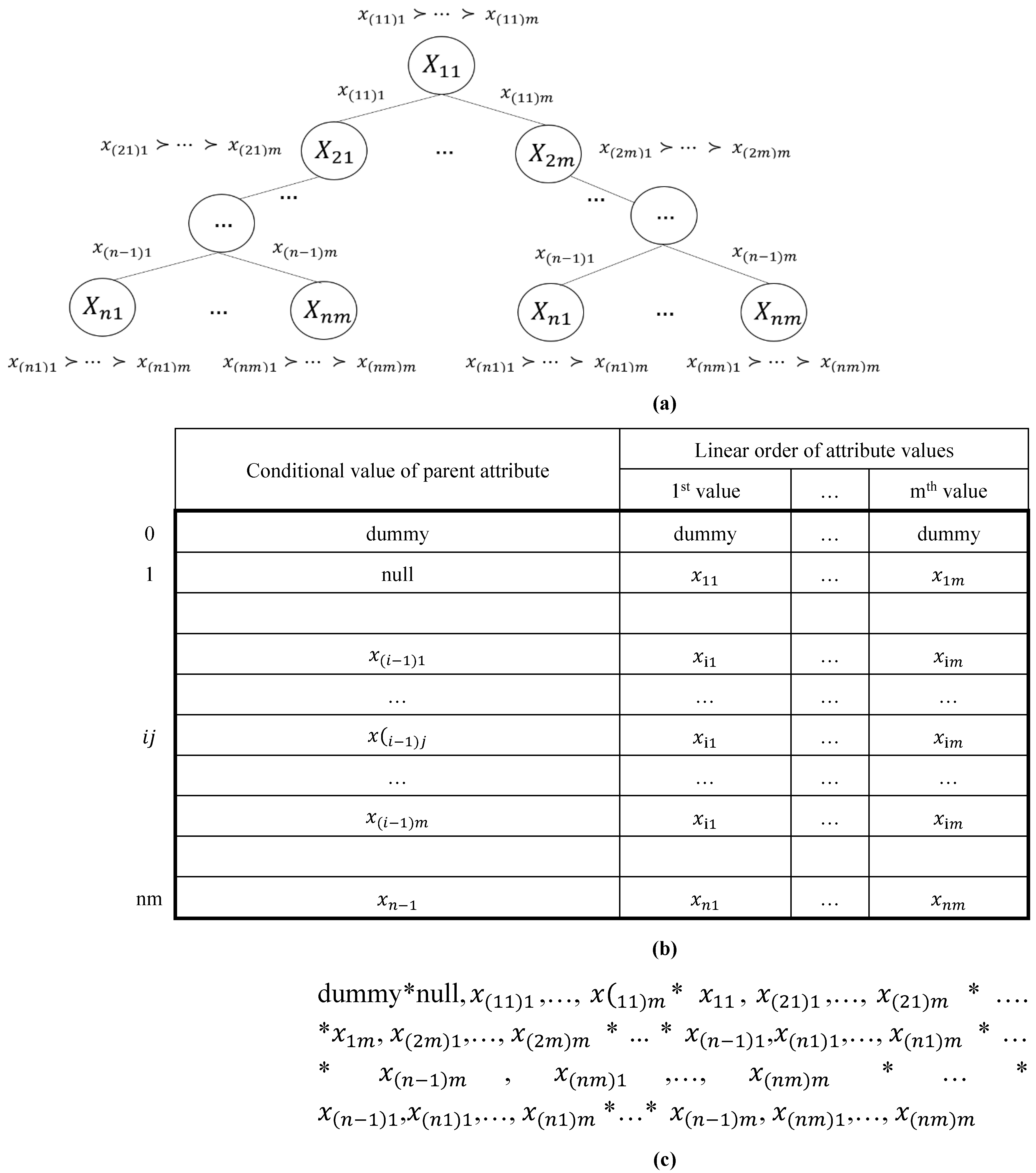
Let the general lexicographic preference tree
(Figure 5a) with at most
attributes (
), each attribute has at most
values (
), is a tree with the depth of at most
, which is shown in an array with
columns and
rows in
Figure 5b. Its string representation also has
parts, each of length
(
Figure 5c). The left branch of the tree contains the best preferences of the user.
In principle, array rows are interdependent and inserted conditionally relative to each other. The structure used is the same as a heap (with offset), where the children of node , whose conditional parent value is at location (i.e. the column 0 in the array representation), are placed at locations to (i.e. the columns 1 to in the array) according to their priorities. In string representation, the nodes are separated by “*”, and the conditional values of each node are separated by “,”.
In general, it can be said that each part in an array or any part in a string can have three states: 1) ‘dummy’, 2) unconditional: ‘null’ 3) conditional. Rules for generating an array are defined as follows:
Row 0 of the array is always assumed to be ‘dummy’.
-
The children of each node in the tree are placed in the rows after this node, according to the number of its attribute values. They also have several states:
The node can have no children: Therefore, its children are ‘dummy’. In this case, the node is called a leaf. So, it can be said that if the left child of the node is ‘dummy’, then the other children must have been ‘dummy’.
The node can be considered unconditionally: In this case, only the left child of the node is set, the conditional parent value also is set as ‘null’, and the other children are ‘dummy’. Because the conditional node only includes the left child.
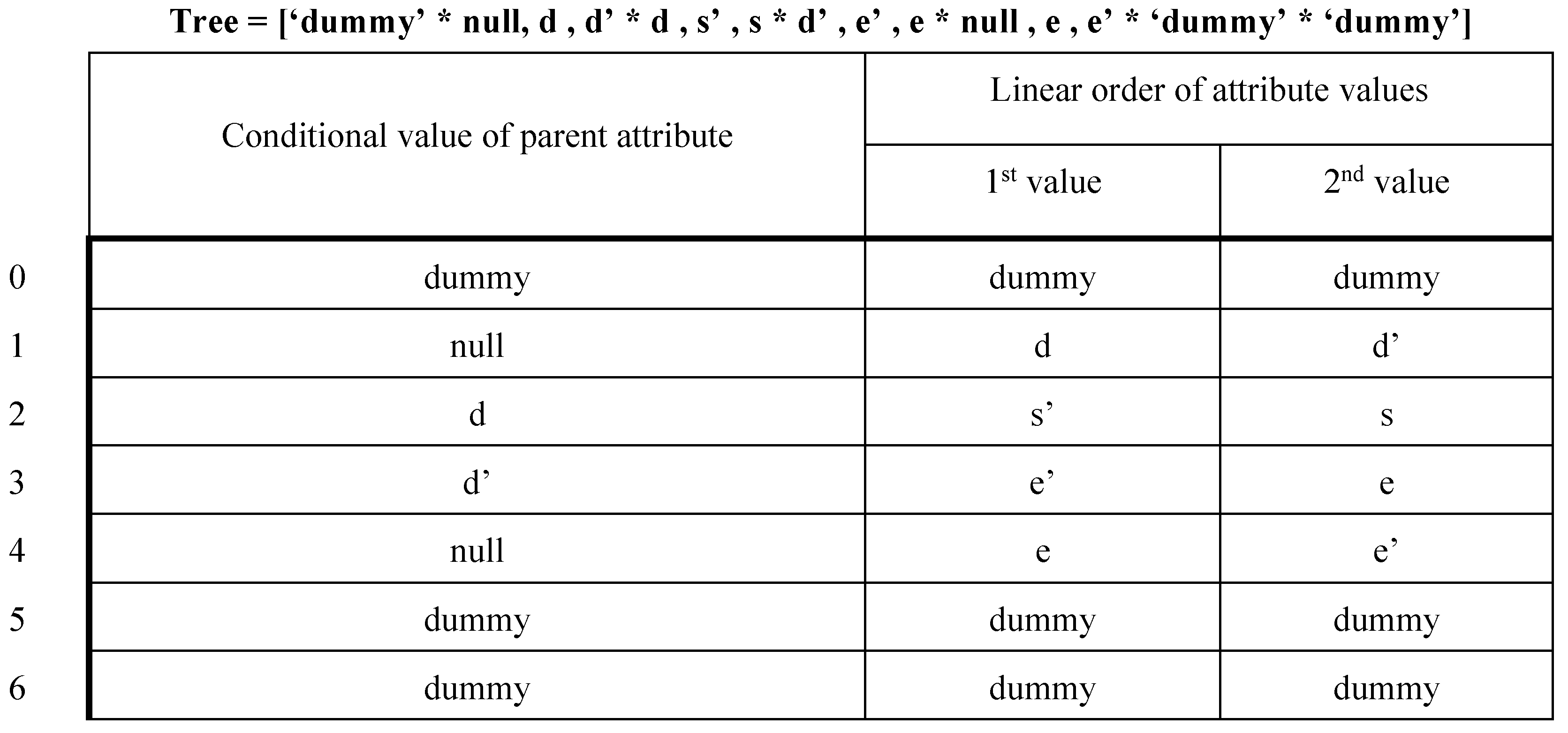
By limiting the general representation, we implement the binary lexicographic preference tree (i.e., for the binary attributes) in array representation as follows:
In row 0, the array is always ‘dummy’.
In other rows, if a node is in -th row of the array, the left child is in and the right child is in .
-
Now, each row of the array itself contains three parts, such that in the first cell the parent node’s conditional value is located. The second and third cells correspond to the priority of the values of each attribute. The second cell is the value that is preferred over the third one. More precisely:
When there is no node (for example, the root parent or the missing child), it is ‘dummy’.
When a node is unconditional, in the first cell of the row is ‘null’.
When a node is conditional, then the value of the parent condition is placed in the first cell of each row.
Figure 6 illustrates the array and string representation of the binary PLP-tree shown in
Figure 2b.
4. Illustration, Experiment, and Discussion
To validate our methodological framework, we conducted a series of experiments applying PLPSim (and other similarity/distance measures, CPSim, LPDis, and PLPDis), coalition formation algorithms (HRECS1, HRECS2, and HRECS3), lexicographic contracts (CLF, CFB, CFW, CFA, CFP) to a hybrid renewable energy tariff case study.
The experimental setup and components used include synthetic consumer preference data expressed as PLP-Trees, supplier tariff structures with hard and soft constraints, and coalition thresholds reflecting group discount conditions. They are close to the reality of the hybrid renewable energy market; some of our experimental settings and assumptions were designed to closely approximate a realistic hybrid renewable energy market.
Outcomes are assessed using both established measures (nDCG, Davies–Bouldin dispersion) and our proposed F@LeX metric, enabling a comprehensive comparison of coalition quality and preference satisfaction.
We demonstrate the asymmetric property of PLPSim in
Section 4.1, show synthetic PLP-tree dataset generation in
Section 4.2, set up the experiments in
Section 4.3, illustrate graphs comparing metric scores across experiments in a case study in hybrid renewable energy tariffs in
Section 4.4, and discuss a summary of findings in
Section 4.5.
4.1. Step-by-Step Example: PLPSim Asymmetry
This example illustrates Theorems 1 and 2 and shows that measuring similarity in combinational settings is asymmetric. This means that due to the existence of attributes or their domain values that may not be shared between the two LP-trees (or for example, in one direction, one is a subset of the other, but in the other direction, the other is not a subset of the same LP-tree), it cannot be said that if the first is similar to the second to a certain degree, the second is necessarily also similar to the first to the same degree.
The
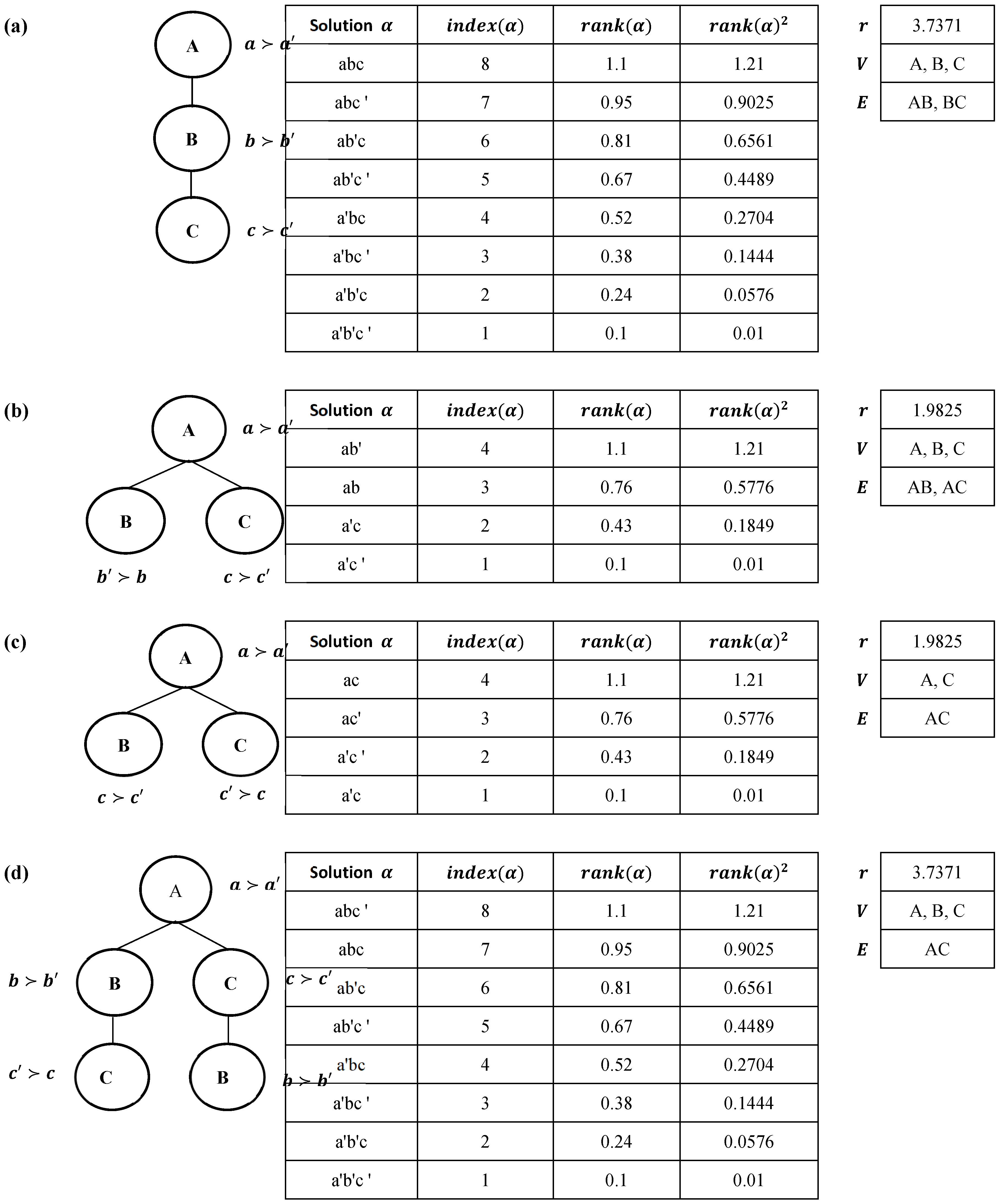
of a consumer preference and a supplier tariff can be in either a complete (CLPT) or a partial (PLPT) structure. Given the lexicographic preferences of a consumer and a supplier tariff represented in
Figure 7a –
Figure 7d, and peripheral calculations of solution ranks in
Figure 8, calculation of the PLPSim similarity score between their corresponding LP-trees follows one of the following comparisons:
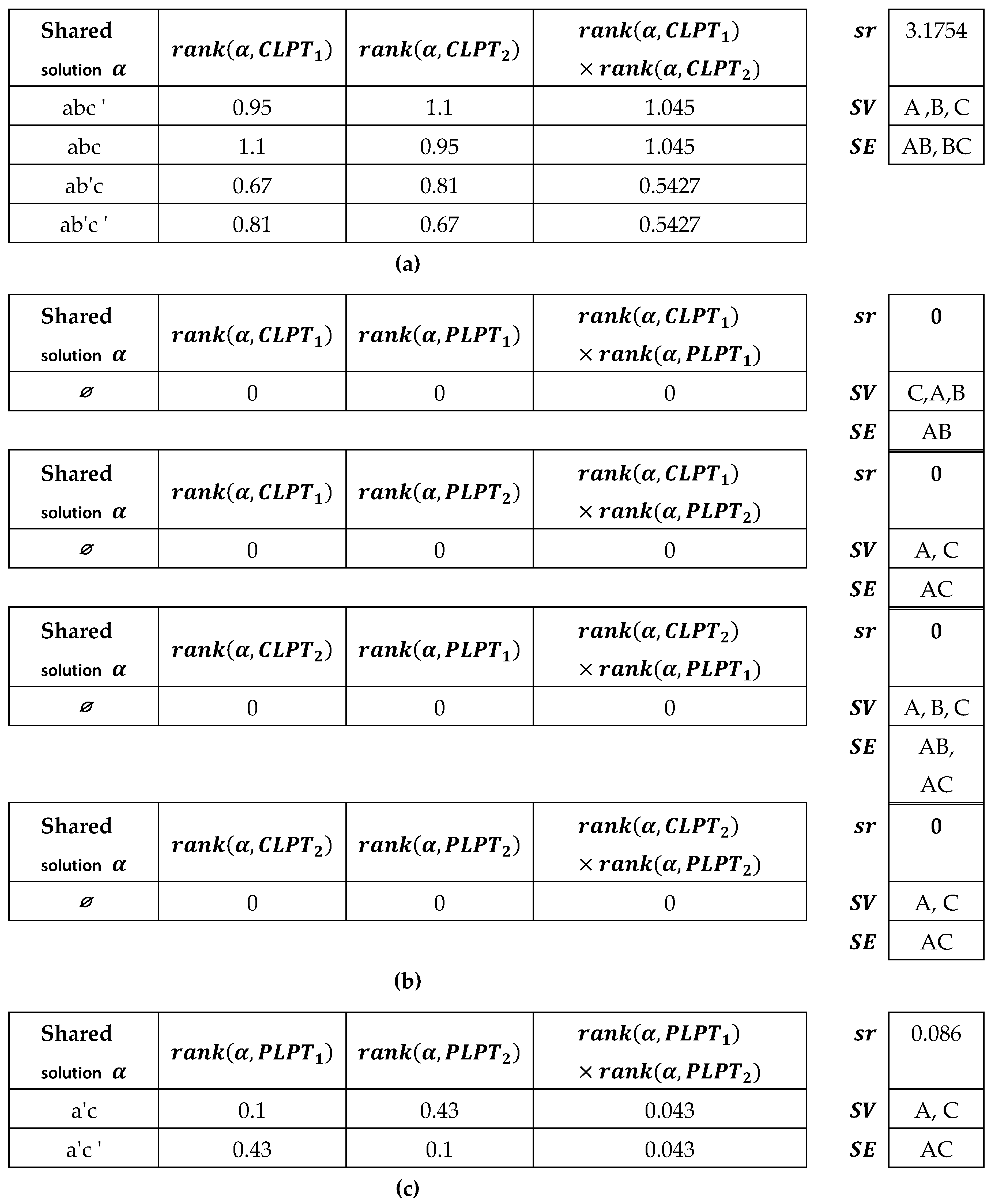
Although the same relative similarity score is obtained in some of the permutations, their calculations show differences and therefore the asymmetry of PLPSim across
or
(complete) and
or
(partial):
For comparison, the information of the first tree is placed in the denominator of the fractions, such that in the first comparison, the number of attributes of the first tree is 3 (A, B, C), the number of edges (AB, AC) is 2, and the number of terms in common with the second tree is 2 according to its table. For the fractions, the number of attributes in common between the two trees is 2 (A, C), the number of common edges is 1 (AC), and the number of shared terms is 2.
is the sum of the product of values of shared solutions; (a) CLPT-CLPT category, (b) CLPT-PLPT and PLPT-CLPT categories, (c) PLPT-PLPT category; = Fig7a (Complete), = Fig7d (Complete), = Fig7b (Partial), = Fig7c (Partial).
4.2. Case Study: Hybrid Renewable Energy Tariffs
As an illustrative application, we contextualize the framework in hybrid renewable energy markets, where consumer PLP-Trees represent tariff preferences and supplier contracts define pricing strategies. Coalitions are formed using PLPSim, and contracts are applied to allocate tariffs. This case study demonstrates the practical utility of the framework while underscoring its generalizability to other multiagent domains.
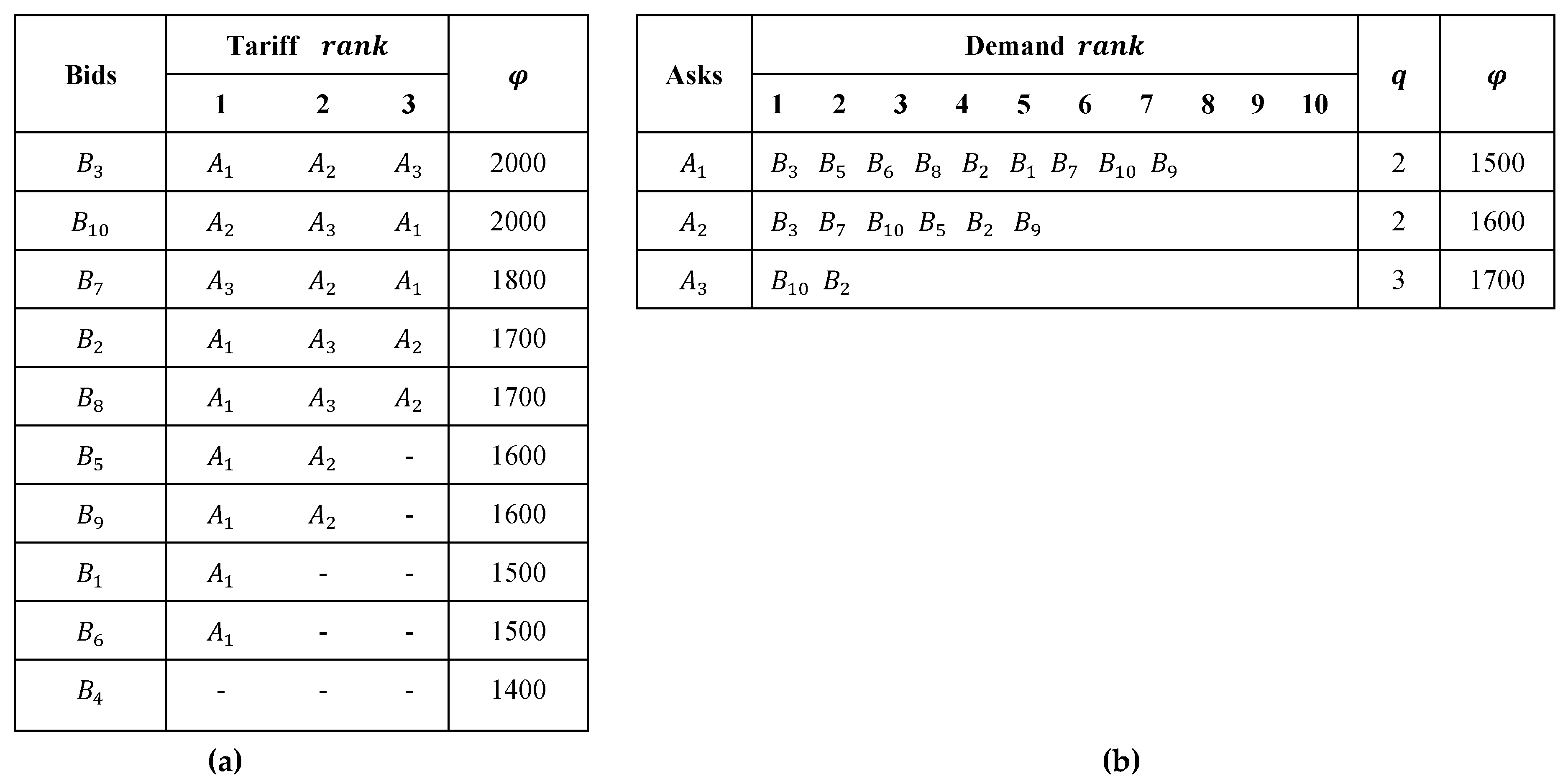
In a hybrid renewable energy market, three lexicographic preference tariffs of energy suppliers and ten lexicographic preference demands of consumers are tabulated in
Table 2 using representations presented in
Section 3.6. Consumer and supplier preferences are listed in
Figure 9 by applying the PLPSim similarity method. The matrix
where the demands
of consumers who have offered a price higher than or equal to the minimum bid price are tabulated in a similar order for each tariff
,
Figure 9a. Matrix lines are in ascending order of tariff prices. The matrix
, where the tariff
of suppliers that have given a price lower than or equal to the maximum price offered by the consumer are tabulated in
Figure 9b, in the order of priority of similarity for each demand
. The rows of this matrix are arranged in descending order of the price of demand; similarity measurements are performed to obtain these two matrices in two directions, and one cannot be obtained from the other.
The tariff selection methods then determine the tariff and contract price for consumers and suppliers from the groups formed on each tariff of these two matrices. Tariff selection is made by combining the three HRECS1, HRECS2, and HRECS3 methods (to form a consumer coalition, Algorithms 1-3) and five methods, CLF (ContractLex + PriceLexFixed), CFB, CFW, CFA, and CFP (to determine the contract and transaction price,
Section 3.4.1 and
Section 3.4.2). The details of the contracts concluded by combining coalition methods and tariff selection methods for consumers similar to each tariff by PLPSim are tabulated in
Table 3.
4.3. Experimental Setup
To evaluate the proposed approach (PLPSim, HRECSs, ContractLex, PriceLex), we designed a controlled experimental environment that integrates both synthetic preference data and real-world tariff scenarios. The setup ensures reproducibility and allows systematic comparison across coalition formation strategies. Two complementary data sources were employed.
We implemented our method in Python and performed the experiments on Google Colab (
https://colab.research.google.com),
Table 4. We generated synthetic preference profiles using PLPGen (Appendix) to capture heterogeneity in consumer lexicographic preferences and supplier tariff structures drawn from the hybrid renewable energy case study introduced in Section 4.2 for different numbers of attributes and values. Together, these datasets ensured that the experiments reflected both theoretical diversity and real-world market conditions. Lexicographic preferences can be either conditional, unconditional, or both along the branches of the trees representing the preferences. Based on the number of parameters (i.e., the decision attributes), the trees are generated in a depth of at most this number. LP-trees including nodes corresponding to any number of attributes and values are generated for making either CLP- or PLP-trees. To be comparable, the decision attributes on both sides of the market are the same. Due to computational limitations and without losing the generality of the proposed methods, tests are run with binary attributes' values.
We run two types of experiments in these markets. In the first, the PLPSim similarity method presented in
Section 3.2 is compared with LPDis, CPSim, and PLPDis methods in terms of time, memory, and processing consumption, and in the second, the performance of PLPSim for consumer grouping and the performance of different coalitions (
Section 3.3), together with the proposed tariff contracts (
Section 3.4), are compared across the synthetic data in terms of different criteria introduced in
Section 3.5.
This setup provides the methodological foundation for analyzing coalition performance under diverse market conditions. The results of these experiments are presented in Section 4.4.
4.3.1. Experiment I: PLPSim Computational Performance
In the first test, all the data of lexicographic preferences with 2 to 5 attributes are applied. These preferences are similarly measured by the PLPSim, CPSim, LPDis, and PLPDis methods. Lexicographic preferences data are complete and incomplete. The count of attributes of preferences on both sides must be the same because the parties' views must be expressed on a set of specific and identical attributes to be comparable.
Table 7 demonstrates specification of the synthetic dataset which address simple to complex markets.
Due to Colab memory limitations (Table 4), all lexicographic preference data are generated by up to 4 binary attributes. It was not possible to load all lexicographic preference (binary) data with 4 attributes and above onto Colab. For 4 attributes, the size of all complete and complete/partial data was 1.4 GB and 3.2 GB, respectively. Since the number of trees gets exponentially large, to be manageable regarding the memory size, we limited the total number of trees per each number of attributes. Hence, for 4 and 5 attributes, 4000 random synthetic lexicographic preferences were generated from each. Moreover, for 2 attributes, the partial lexicographic preference tree (i.e., with 1 attribute) is not defined. For the set containing both complete and partial lexicographic preferences, the same complete set is used for the other side of the test.
Table 5 expresses the proportion of the number of complete and partial preferences that it generates.
4.3.2. Experiment II: PLPSim Performance in Group Tariff Selection
In this experiment, we contrast PLPSim with PLPDis existing method for comparing partial lexicographic preferences in coalition formation of consumers for suppliers’ tariffs. This second test is run on 27 synthesized energy markets, including all 2 to 10 complete lexicographic tariffs and 10 to 1000 partial lexicographic preferences of consumers over 2 to 4 binary attributes,
Table 6 and
Table 7. In each test, the count of consumer groups remains constant and equal to the count of tariffs offered in the market. Here, first, the PLPSim and PLPDis similarity methods applied to complete and partial lexicographic preferences are compared in scenarios based on various attributes of lexicographic preferences, the count of tariffs offered by suppliers, and the count of energy consumer demands. The results are evaluated through the Davies-Bouldin dispersion index (the less, the better; Definition 10) and Normal Discounted Cumulative Gain (nDCG; closer to 1, the better; Definition 11) and are compared with PLPDis performance. We also employ our proposed F@Lex metric (Definitions 12—15) to focus on performance of PLPSim for selecting different contracts in coalition formation systems (presented in
Section 3.4 and
Section 3.3, respectively).
Table 8 lists these combinations, totally resulting in 162 experiment scenarios.
Table 6.
Specification of Experiment II dataset for market setting regarding the number of attributes, tariffs, and consumers.
Table 6.
Specification of Experiment II dataset for market setting regarding the number of attributes, tariffs, and consumers.
| Market |
1 |
2 |
3 |
4 |
5 |
6 |
7 |
8 |
9 |
10 |
11 |
12 |
13 |
14 |
15 |
16 |
17 |
18 |
19 |
20 |
21 |
22 |
23 |
24 |
25 |
26 |
27 |
| #Attributes |
2 |
2 |
2 |
2 |
3 |
3 |
3 |
3 |
3 |
3 |
3 |
3 |
3 |
4 |
4 |
4 |
4 |
4 |
4 |
4 |
4 |
4 |
4 |
4 |
4 |
3 |
4 |
| #Tariffs |
2 |
2 |
5 |
5 |
2 |
2 |
2 |
5 |
5 |
5 |
10 |
10 |
10 |
2 |
2 |
2 |
5 |
5 |
5 |
10 |
10 |
10 |
20 |
20 |
20 |
50 |
50 |
| #Consumers |
10 |
16 |
10 |
16 |
10 |
100 |
1000 |
10 |
100 |
1000 |
10 |
100 |
1000 |
10 |
100 |
1000 |
10 |
100 |
1000 |
10 |
100 |
1000 |
10 |
100 |
1000 |
1000 |
1000 |
Table 7.
Specification of Experiment II dataset for market setting regarding price range.
Table 7.
Specification of Experiment II dataset for market setting regarding price range.
Suppliers tariff price
(currency/kWh) |
Quorum for group discount |
Consumers bid price
(currency/kWh) |
| 1000 4000 |
5 20 |
1500 3000 |
Table 8.
Lexicographic similarity measurement methods and group tariff selection in Experiment II.
Table 8.
Lexicographic similarity measurement methods and group tariff selection in Experiment II.
| Similarity method |
PLPDis |
PLPSim |
| Coalition method |
HRECS1 |
HRECS2 |
HRECS3 |
| Tariff contract |
CFB |
CFA |
CFW |
CFP |
4.5. Experimental Results
Experiments were conducted across distinct market scenarios, encompassing varying scales of consumer populations, ranging from small groups of 10–20 participants to larger markets with more than 200 consumers, tariffs, and prices. The results provide a comprehensive view of how the proposed PLPSim, ContractLex, and PriceLex perform under diverse HRECS coalition formation settings.
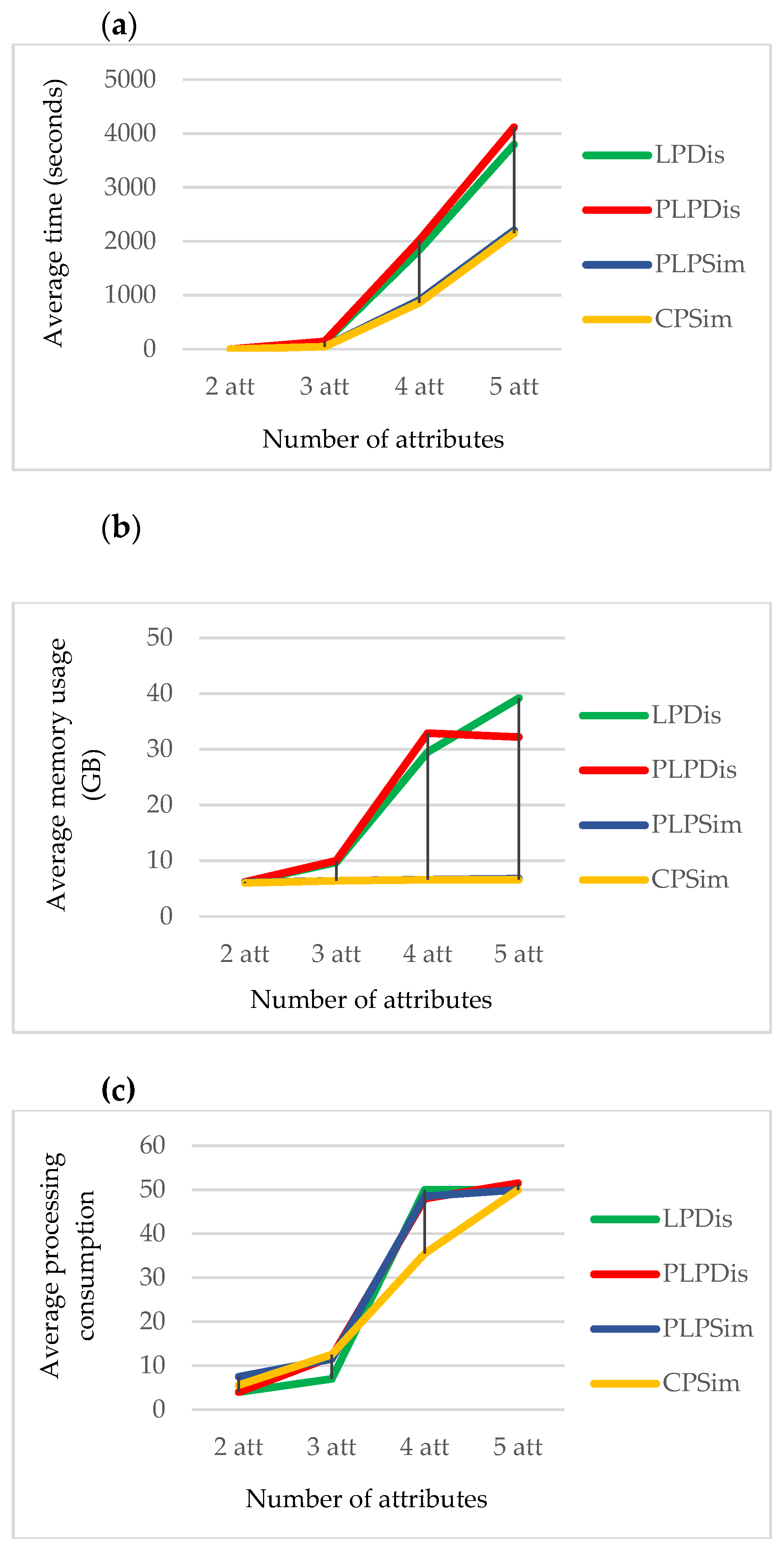
According to
Figure 10, the family simulation methods and Kendall-based distance sensing methods (LPDis and PLPdis) consume more processing time and memory. There exists a direct relation between the count of attributes of lexicographic preferences and the computational complexity of all methods. The PLPSim method outperforms its counterparts in all three criteria, DB, nDCG, and F@Lex.
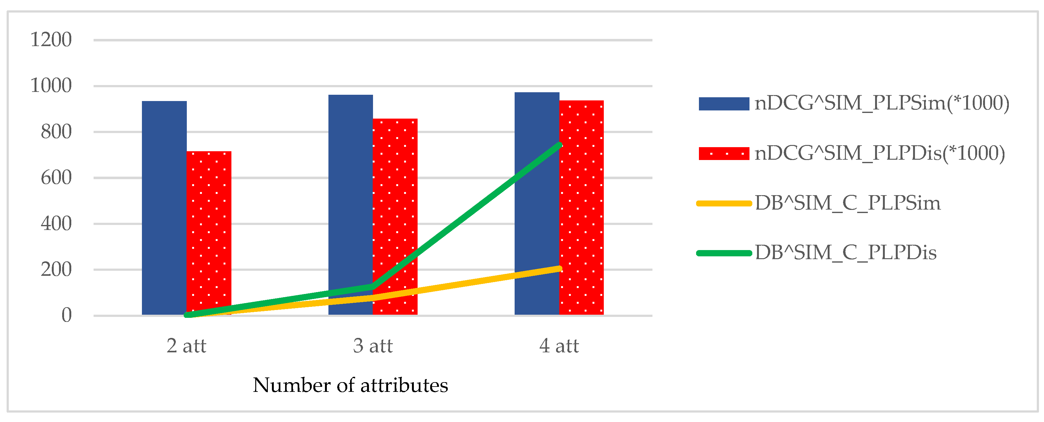
As observed in
Figure 11, an increase in the count of attributes increases the Davis-Bouldin index of PLPSim and PLPDis methods, where PLPDis yields a higher average. The PLPSim method maintains the quality by increasing the count of attributes, on average. PLPSim outperforms PLPDis in two other HRECSs that focus on consumers only or all parties.
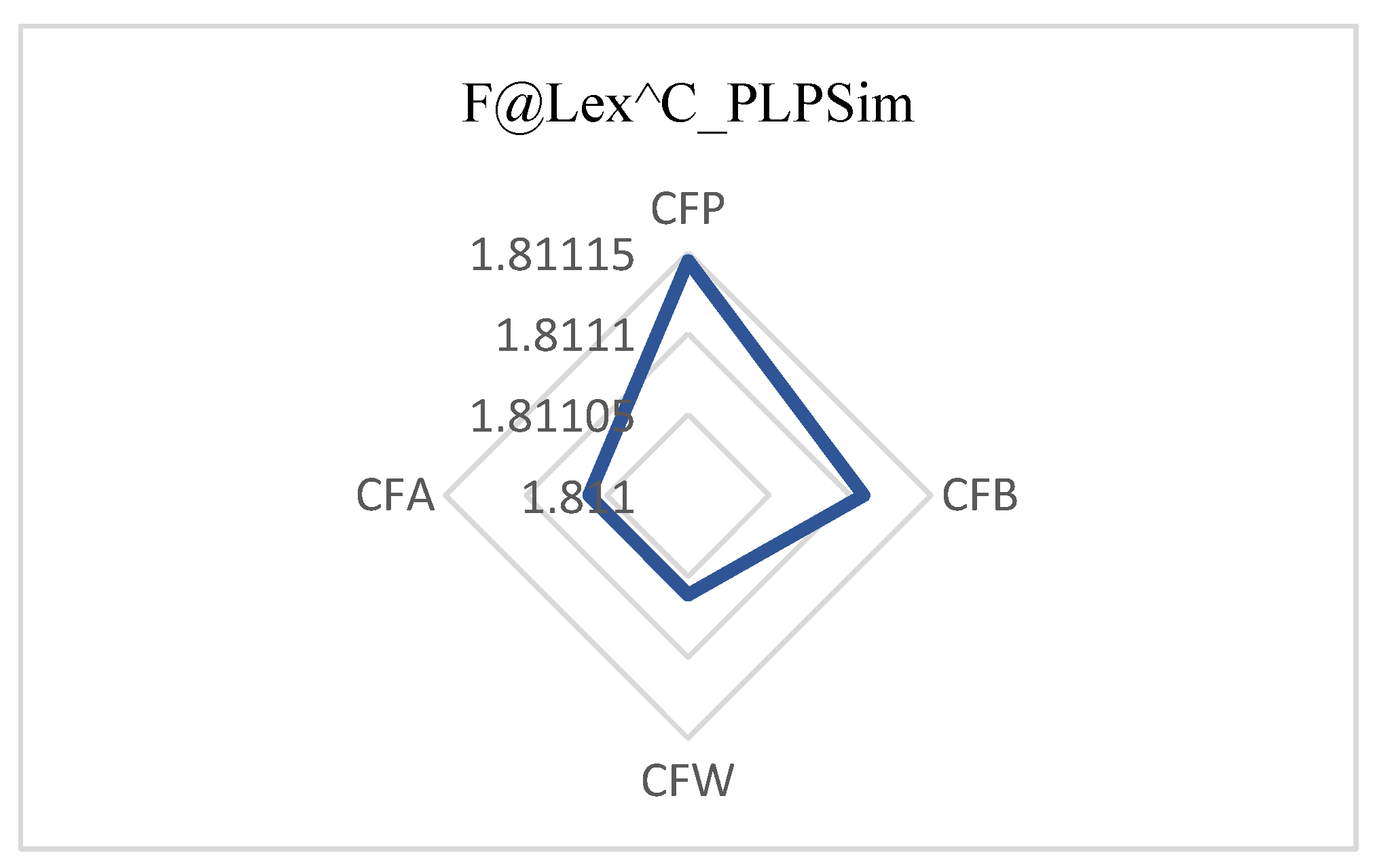
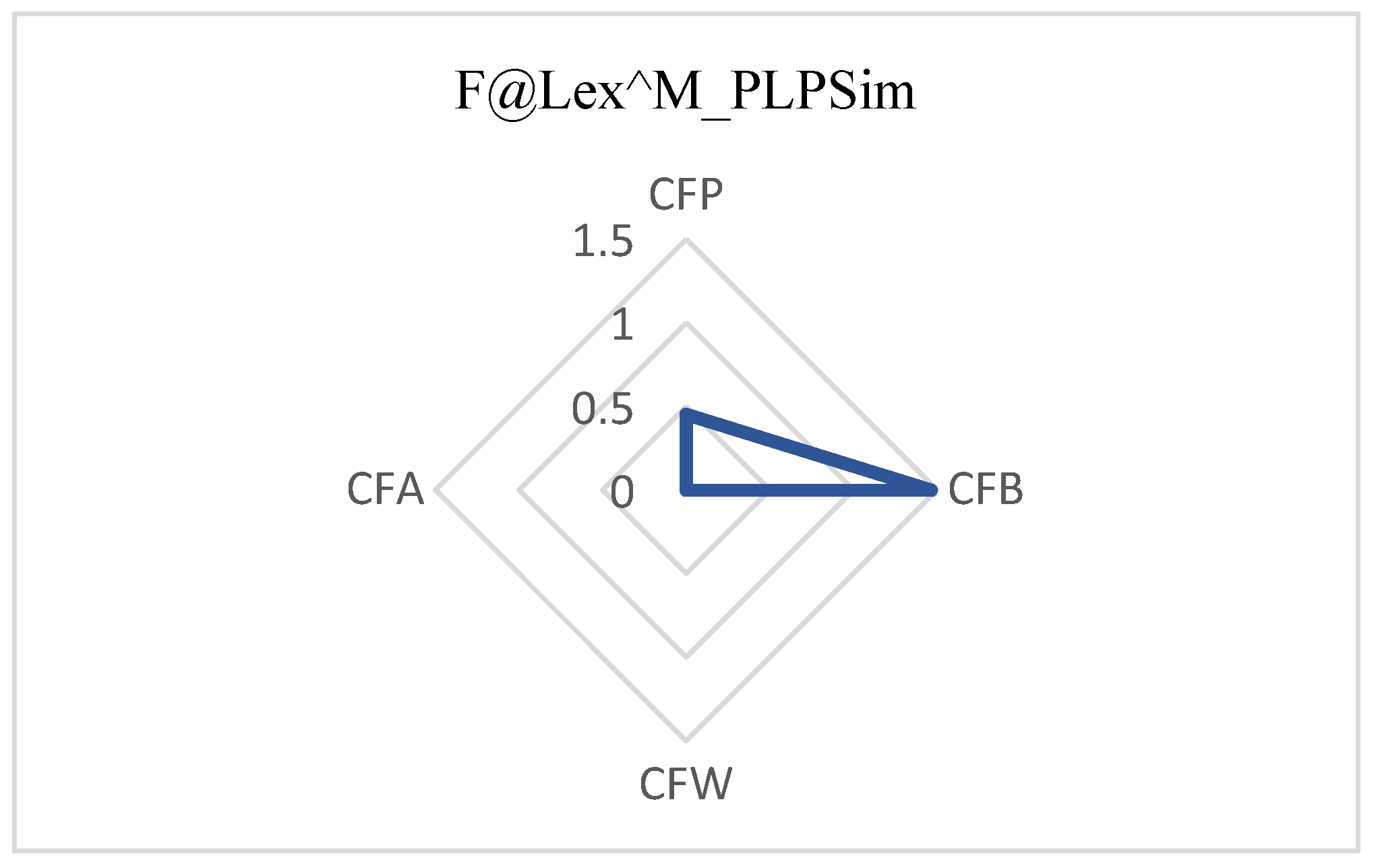
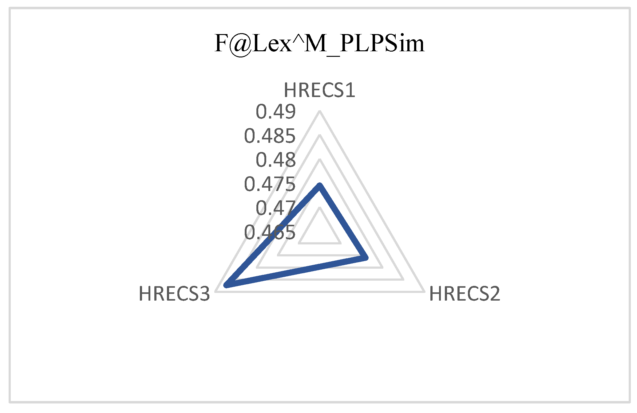
The F@Lex satisfaction criteria (Definitions 12 to 15) indicate the appropriateness of the contract for the defined parties; that is, the contract that results from implementing the combination of the tariff selection protocol, the coalition formation method, and the similarity method, reveals its effect on consumer and supplier satisfaction as an F-measure. For this purpose, any contract and other solutions related to a lexicographic preference, with degrees based on their rank, are placed in more than one category. Different protocols lead to different satisfaction for consumers and suppliers. The F-measure is a number between 0 and 1, and the closer to 1 it is, the better. According to Figures 12—14, it can be deduced that CFP, CFB, CFW, and CFA contracts are appropriate for consumers, respectively, and CFB is appropriate for both consumers and suppliers. The HRECS3 coalition method is better than other coalition methods.
4.4. Findings and Policy Implications,
The evaluation of the proposed methods and protocols reveals several important insights into scalability, similarity performance, coalition efficiency, contract profitability, error minimization, and F-measure outcomes. These findings collectively demonstrate how methodological choices influence consumer welfare, supplier benefits, and overall societal outcomes across different coalition and contract settings:
Runtime scalability: PLPSim exhibits linear growth in runtime and scalability with increasing numbers of features (
Figure 10a).
Memory efficiency: PLPSim is more scalable in terms of memory consumption as the number of features increases (
Figure 10b).
Similarity performance: PLPSim achieves more favorable nDCG similarity than PLPDis for preferences with fewer facets (
Figure 11).
Coalition efficiency: PLPSim is more efficient in symmetric coalition methods (HREC3), while PLPDis efficiency decreases (
Figure 11).
Consumer similarity index: HRECS3 coalition formation yields the smallest Davis–Bouldin index of consumer similarity (
Figure 11).
Consumer F-measure: CFP protocol produces the best F-measure for consumers (
Figure 12).
Supplier F-measure: CFB protocol yields the best F-measure for suppliers and, on average, for society (
Figure 13).
Alternative supplier F-measure: HRECS3 produces the best F-measure for suppliers and, on average, for society (
Figure 14).
PLPDis comparative performance: PLPDis similarity method achieves slightly better F-measure than PLPSim for consumers, suppliers, and society (
Figure 14).
Briefly, the evaluation results indicate that HRECSs combined with any contract protocol employing PLPSim outperform those applying the PLPDis method in terms of Normalized Discounted Cumulative Gain (nDCG) and intra- and inter-group Davies–Bouldin dispersion. With respect to F@LeX, the selection of tariffs adopting HRECS3 + CFP yields the highest satisfaction for consumers, whereas HRECS3 + CFB provides the greatest satisfaction for both parties. The observed improvements in nDCG and F@LeX (F-measure) are not merely statistical; they reflect meaningful advancements in complex markets, including the hybrid renewable energy market case study.
Higher nDCG scores indicate that the most relevant tariffs (i.e., those closely aligned with consumer preferences) are ranked higher in the recommendation list. In practice, this means that:
Consumers are more likely to encounter tariffs that match their needs early in the selection process.
Decision fatigue is reduced and satisfaction increased, as users spend less time evaluating irrelevant options.
Trust in the system’s ability to reflect individual priorities is improved, which can boost adoption rates of HRES.
Improved F-measure, which balances precision and recall, reflects a more accurate and comprehensive matching between consumer bids and supplier offers. This leads to:
More successful coalition formations, as consumers are grouped with others who share similar preferences.
A higher likelihood of meeting supplier quorum thresholds, unlocking group discounts and lowering energy costs.
Enhanced supplier profitability and consumer retention, due to better alignment of expectations and outcomes.
Together, these metrics translate into real-world gains—enhancing market efficiency, boosting consumer satisfaction, and strengthening supplier competitiveness—that are especially vital in decentralized energy systems.
5. Conclusions and Future Works
We introduced PLPSim similarity measurement method, which distinguishes asymmetry in comparing complete or partial lexicographic preferences. To group the consumers concerning renewable energy by applying the most appropriate tariff at a discounted cost, the degree of similarity of lexicographic preferences is applied to calculate the proposed PLPSim and form a group purchase coalition and contract allocation. To operationalize coalition agreements, we defined five types of lexicographic contracts (CLF, CF, CFW, CFA, and CFP), which are applied within three proposed HRECS coalition systems to determine outcomes that maximize fairness and efficiency. In this process, the most appropriate tariff is selected for each consumer. The objective is to provide a planning method for purchasing hybrid renewable energy to manage consumption in smart grids and form a coalition of hybrid renewable energy consumers based on the similarity of preferences and tariff selection. We evaluated our approach vs. existing methods (CPSim, LPDis, and PLPDis) using Davis-Bouldin, nDCG, and proposed F@Lex in coalition formation. Due to the lack of a real-world PLP-tree dataset, we presented PLPGen for generating such synthetic data. According to the evaluation methods over a variety of energy market scenarios, it is possible to adopt the proposed PLPSim method next to different coalition methods and determine the contract protocol in terms of execution time, memory, dispersion, and the essential factor, mutual satisfaction.
In future work, in addition to evaluating these available solutions, the attributes and edges of the LP-tree can be ranked in the PLPSim similarity method, and the percentage of completeness of the solutions and varying pricing conditions can affect the degree of similarity of the lexicographic preferences tree and robustness of coalitions. Similar to CPSim [
16], we balanced the weights of components for shared variables, edges, and rank products in Equation (3). A future study could conduct sensitivity analyzes to determine how variations in these weights affect coalition formation outcomes. Although the string and array implementations of the methods bring the fastest calculations for lexicographic representation, specific algorithmic optimizations for functioning in metropolitan-scale energy markets could be the subject of a future study. The reputation of energy suppliers could be considered as their priority for allocating their tariffs to consumers in meeting their consumers' demands. The interdisciplinary nature of this subject allows for innovative solutions that could significantly impact the future of energy consumption and sustainability. Future research could benefit from combining coalition-based tariff personalization with broader market and policy frameworks. Integrating lexicographic preference coalition models with economic efficiency assessments may ensure both consumer satisfaction and financial sustainability [
8]. At the same time, exploring synergies with adaptive optimization strategies—drawing on evolutionary game theory and reinforcement learning—could enhance responsiveness to dynamic market conditions [
9,
14]. Incorporating risk-sharing support schemes may provide a pathway to balance consumer preference aggregation with macro-level risk management, reducing tariff deficits while maintaining investment incentives [
10]. Extending coalition-based models to interact with hybrid renewable energy system optimization approaches could further improve system-level efficiency and resilience [
11]. Building stronger connections with game-theoretical analyses of electricity markets would reinforce the strategic and policy relevance of coalition models [
13]. Taken together, these directions highlight the potential for a unified framework that bridges consumer-centric coalition models with adaptive, sustainable energy market policies.
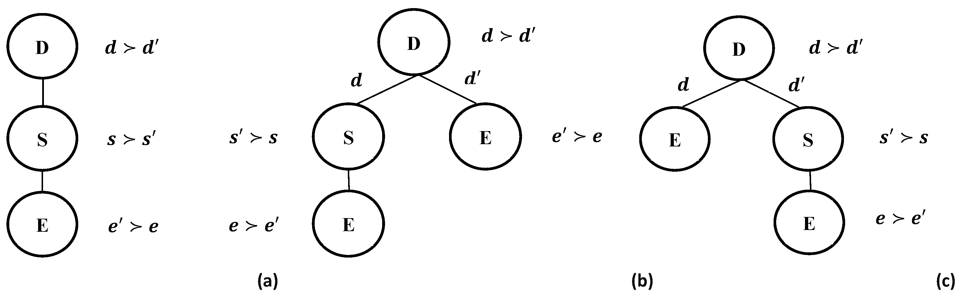
Figure 2.
(a) A Complete LP-tree, (b) A Partial LP-tree, (c) Changing the order of solutions of LP-tree 2b.
Figure 2.
(a) A Complete LP-tree, (b) A Partial LP-tree, (c) Changing the order of solutions of LP-tree 2b.
Figure 4.
Relative interleaved turns between two ordered matrices and contain ordered lists of consumers similar to tariff preferences and ordered lists of tariffs similar to consumers' preferences.
Figure 4.
Relative interleaved turns between two ordered matrices and contain ordered lists of consumers similar to tariff preferences and ordered lists of tariffs similar to consumers' preferences.
Figure 5.
Representation of the general lexicographic preference tree with attributes and $m$ values, (b) Array representation of the lexicographic preference tree , (c) String representation of the lexicographic preference tree .
Figure 5.
Representation of the general lexicographic preference tree with attributes and $m$ values, (b) Array representation of the lexicographic preference tree , (c) String representation of the lexicographic preference tree .
Figure 6.
Binary lexicographic preference tree representation with conditional string and array from the tree in
Figure 2b.
Figure 6.
Binary lexicographic preference tree representation with conditional string and array from the tree in
Figure 2b.
Figure 7.
Score of solutions for multiple lexicographic preferences with 3 attributes, where is the sum of squared values of solutions, and and are respectively the vertices and edges of the LP-trees; (a) Complete: UI-UP, (b) Partial: CI-UP, (c) Partial: CI-CP, and (d) Complete: CI-CP.
Figure 7.
Score of solutions for multiple lexicographic preferences with 3 attributes, where is the sum of squared values of solutions, and and are respectively the vertices and edges of the LP-trees; (a) Complete: UI-UP, (b) Partial: CI-UP, (c) Partial: CI-CP, and (d) Complete: CI-CP.
Figure 8.
Intermediate calculations for PLPSim similarity of the four lexicographic preference trees of , where
Figure 8.
Intermediate calculations for PLPSim similarity of the four lexicographic preference trees of , where
Figure 9.
An ordered matrix based on price , (a) contains ordered lists of Tariffs preferences similar to the demands of consumers, (b) contains ordered lists of preferences of consumers similar to the tariffs .
Figure 9.
An ordered matrix based on price , (a) contains ordered lists of Tariffs preferences similar to the demands of consumers, (b) contains ordered lists of preferences of consumers similar to the tariffs .
Figure 10.
Consumption of computational resources as average to run similarity methods LPDis, PLPDis, CPSim, and PLPSim according to the number of attributes of lexicographic preferences (a) time (s), (b) memory (gigabytes), and (c) processing.
Figure 10.
Consumption of computational resources as average to run similarity methods LPDis, PLPDis, CPSim, and PLPSim according to the number of attributes of lexicographic preferences (a) time (s), (b) memory (gigabytes), and (c) processing.
Figure 11.
PLPSim and PLPDis’s nDCG and Davies-Bouldin index of consumer's lexicographic preferences with 2—4 attributes.
Figure 11.
PLPSim and PLPDis’s nDCG and Davies-Bouldin index of consumer's lexicographic preferences with 2—4 attributes.
Figure 12.
Consumers’ F@Lex (satisfaction) for tariff contracts CFP, CFA, CFW, and CFB with the PLPSim method.
Figure 12.
Consumers’ F@Lex (satisfaction) for tariff contracts CFP, CFA, CFW, and CFB with the PLPSim method.
Figure 13.
The social satisfaction (F@Lex) for tariff contracts CFP, CFA, CFW, and CFB with the PLPSim method.
Figure 13.
The social satisfaction (F@Lex) for tariff contracts CFP, CFA, CFW, and CFB with the PLPSim method.
Figure 14.
The social satisfaction (F@Lex) for coalition formations HRECS1, HRECS2, and HRECS3 with the PLPSim method.
Figure 14.
The social satisfaction (F@Lex) for coalition formations HRECS1, HRECS2, and HRECS3 with the PLPSim method.
Table 1.
Comparison of similarity of lexicographic preference tress of
Figure 2 by
PLPSim,
CPSim,
LPDis, and
PLPDis.
Table 1.
Comparison of similarity of lexicographic preference tress of
Figure 2 by
PLPSim,
CPSim,
LPDis, and
PLPDis.
| PLPDis distance |
LPDis distance |
CPSim similarity |
PLPSim similarity |
Lexicographic preferences |
| 10 |
7 |
0.833 |
0.906 |
Figure 2a andFigure 2b |
| 8 |
5 |
0.833 |
0.698 |
Figure 2a andFigure 2c |
Table 2.
Three complete binary lexicographic preference tariffs from 2 suppliers and complete binary lexicographic preferences demand from 10 consumers.
Table 2.
Three complete binary lexicographic preference tariffs from 2 suppliers and complete binary lexicographic preferences demand from 10 consumers.
| Partial/Complete Binary Lexicographic Preference (PLP) |
Bid |
Consumer |
| dummy*null,a0,a1*a0,c1,c0*a1,b1,b0*null,b0,b1#1500 |
|
|
| dummy*null,c0,c1*null,a1,a0#1700 |
|
|
| dummy*null,a1,a0*a1,c1,c0*a0,b1,b0*null,b1,b0*dummy*b1,c1,c0*b0,c0,c1#2000 |
|
|
| dummy*null,b0,b1*b0,a0,a1*b1,a1,a0*dummy*dummy*null,c1,c0#1400 |
|
|
| dummy*null,a1,a0*null,b0,b1*dummy*null,c1,c0#1600 |
|
|
| dummy*null,a0,a1*null,b1,b0*dummy*null,c0,c1#1500 |
|
|
| dummy*null,c1,c0*null,b1,b0*dummy*null,a1,a0#1800 |
|
|
| dummy*null,a0,a1*null,b1,b0*dummy*b1,c1,c0*b0,c0,c1#1700 |
|
|
| dummy*null,c0,c1*null,b0,b1#1600 |
|
|
| dummy*null,a0,a1*null,c1,c0*dummy*null,b0,b1#2000 |
|
|
| (Complete) Binary Lexicographic Preference (LP) |
Ask |
Supplier |
| dummy*null,b0,b1*null,c1,c0*dummy*c1,a0,a1*c0,a1,a0#1500#2#1 |
|
|
| dummy*null,c1,c0*c1,b1,b0*c0,a1,a0*null,a1,a0*dummy*a1,b0,b1*a0,b1,b0#1700#3#1 |
|
|
| dummy*null,b1,b0*b1,a1,a0*b0,a0,a1*null,c1,c0*dummy*a0,c0,c1*a1,c1,c0#1600#2#2 |
|
|
Table 3.
Tariff selection for consumer preferences by PLPSim similarity and HRECS1, HRECS2, and HRECS3 coalition formation methods and CLF, CFB, CFW, CFA, and CFP tariff contracts.
Table 3.
Tariff selection for consumer preferences by PLPSim similarity and HRECS1, HRECS2, and HRECS3 coalition formation methods and CLF, CFB, CFW, CFA, and CFP tariff contracts.
| CFP |
CFA |
CFW |
CFB |
CLF |
Demand |
Method |
| Price |
Contract |
Price |
Contract |
Price |
Contract |
Price |
Contract |
Price |
Tariff |
| 1350 |
|
1620 |
|
1620 |
|
1620 |
|
1350 |
|
|
HRECS1 |
| 1440 |
|
1620 |
|
1620 |
|
1620 |
|
1350 |
|
|
| 1850 |
|
2000 |
|
2000 |
|
2000 |
|
1800 |
|
|
| - |
- |
- |
- |
- |
- |
- |
- |
- |
-
|
|
| 1395 |
|
1620 |
|
1620 |
|
1620 |
|
1350 |
|
|
| 130 |
|
1620 |
|
1620 |
|
1620 |
|
1350 |
|
|
| 1750 |
|
2000 |
|
2000 |
|
2000 |
|
1800 |
|
|
| 1440 |
|
1620 |
|
1620 |
|
1620 |
|
1350 |
|
|
| 1395 |
|
1620 |
|
1620 |
|
1620 |
|
1350 |
|
|
| 1800 |
|
2000 |
|
2000 |
|
2000 |
|
2000 |
|
|
| 1350 |
|
1800 |
|
1800 |
|
1800 |
|
1350 |
|
|
HRECS2 |
| 1700 |
|
1700 |
|
1700 |
|
1700 |
|
1800 |
|
|
| 1575 |
|
1800 |
|
1800 |
|
1800 |
|
1350 |
|
|
| - |
- |
- |
- |
- |
- |
- |
- |
- |
-
|
|
| 1395 |
|
1800 |
|
1800 |
|
1800 |
|
1350 |
A1 |
|
| 1350 |
|
1800 |
|
1800 |
|
1800 |
|
1350 |
|
|
| 1530 |
|
1800 |
|
1800 |
|
1800 |
|
2000 |
|
|
| 1700 |
|
1700 |
|
1700 |
|
1700 |
|
1800 |
|
|
| 1440 |
|
1800 |
|
1800 |
|
1800 |
|
2000 |
|
|
| 1620 |
|
1800 |
|
1800 |
|
1800 |
|
2000 |
|
|
| 1350 |
|
1530 |
|
1530 |
|
1530 |
|
1350 |
|
|
HRECS3 |
| 1440 |
|
1530 |
|
1530 |
|
1530 |
|
1350 |
|
|
| 1850 |
|
2000 |
|
2000 |
|
2000 |
|
1800 |
|
|
| - |
- |
- |
- |
- |
- |
- |
- |
- |
-
|
|
| 1395 |
|
1530 |
|
1530 |
|
1530 |
|
1350 |
|
|
| 1350 |
|
1530 |
|
1530 |
|
1530 |
|
1350 |
|
|
| 1485 |
|
1530 |
|
1530 |
|
1530 |
|
1350 |
|
|
| 1440 |
|
1530 |
|
1530 |
|
1530 |
|
1350 |
|
|
| 1395 |
|
1530 |
|
1530 |
|
1530 |
|
1350 |
|
|
| 1850 |
|
2000 |
|
2000 |
|
2000 |
|
1800 |
|
|
Table 4.
Configuration of Google Colab used for experiments.
Table 4.
Configuration of Google Colab used for experiments.
| CPU |
Intel(R) Xenon(R) CPU @ 2.20GHz |
| GPU |
Tesla P100-PCIE-16GB 3584 CUDA cores , 16GB vRAM |
| RAM |
12.6 GB |
Table 5.
Specification of Experiment I dataset for comparing Lexicographic Preferences similarity methods.
Table 5.
Specification of Experiment I dataset for comparing Lexicographic Preferences similarity methods.
| Lexicographic Preference Data |
Number of attributes |
| 2 |
3 |
4 |
5 |
| Count of all complete LP-trees |
16 |
1248 |
4000 |
4000 |
| All complete LP-tree data capacity (KB) |
1 |
93 |
492 |
806 |
| Count of complete/partial LP-trees |
- |
1920 |
4000 |
4000 |
| Complete/partial LP-tree data capacity (KB) |
-
|
103 |
367 |
553 |