
Submitted:
29 December 2025
Posted:
30 December 2025
You are already at the latest version
Abstract
This study investigates how a Long Short-Term Memory (LSTM) model inter-nally represents baseflow contributions in snowmelt-driven, semi-arid mountain basins with heterogeneous geologic characteristics. Five basins in the Sangre de Cristo Mountains of northern New Mexico, spanning fractured Precambrian bedrock and sedimen-tary-volcanic terrain, were used to evaluate both model performance and interpretability. Baseflow dynamics were inferred post hoc using the Baseflow Index (BFI) and a two-reservoir HEC-HMS (Hydrologic Engineering Center’s Hydrologic Modeling System) model. Although baseflow was not explicitly included in model training, internal cell state activations showed strong correlations with both shallow and deep baseflow com-ponents derived from the HEC-HMS model. To better understand how these relationships may change under climatic stress, BFI-based baseflow patterns were further analyzed un-der pre-drought and drought conditions. Results indicate that the LSTM learned to inter-nally distinguish between short- and long-residence flowpaths, encoding physically meaningful hydrologic behavior. This work demonstrates the potential for LSTM models to offer valuable insights into baseflow generation and groundwater–surface water inter-actions, particularly critical in water-scarce regions facing increasing drought frequency.
Keywords:
long short-term memory (LSTM)
; baseflow
; groundwater–surface water interactions
; snowmelt-dominated basins
; hydrologic model interpretability
; HEC-HMS
; mountain hydrology
1. Introduction
In the Southwestern United States, drainage from mountain ranges is a core component of the hydrologic cycle and critical for sustaining the region and meeting water demand [1,2,3,4,5]. In these settings, complex subsurface interactions, driven by fractured bedrock, steep terrain, and localized faulting, govern the movement and timing of groundwater discharge to streams. Groundwater circulates in the bedrock of the mountain block through shallow and deep pathways, maintaining perennial streams through the summer and fall, beyond the snowpack release in the spring [6,7]. Recent studies have shown that it plays a more significant role than previously thought and the groundwater is more actively cycled at deeper depths than the traditional shallow active soil layer commonly employed in numerical and conceptual models [6,7]. While surface and shallow soil responses are often observable through discharge and soil moisture measurements, deeper groundwater pathways remain largely hidden from direct observation [8].
Because of their importance in regional water supplies, accurate modeling of these streams is critical, and because groundwater contributions play a major role, understanding these processes is equally essential. Physically based models are frequently used for hydrological modeling of these systems, but due to the unseen and largely unknown nature of the groundwater pathways and residence time, it is difficult to validate and inform hydrogeologic models of groundwater contribution [3]. LSTM’s have been increasingly popular in recent years for streamflow modeling with promising results [9,10,11]. LSTM’s offer several advantages over physically based hydrologic models, such as the ability to learn and understand the mechanisms driving the hydrologic cycle and replicate real world processes. This enables it to understand aspects such as baseflow contribution without it being explicitly given [12,13]. While there are many studies investigating the performance of these LSTM models, there is little literature exploring how well and to what degree these models can internalize and understand baseflow dynamics and groundwater contributions in geologically complex, snowmelt driven, mountainous basins.
This study explores the ability of an LSTM models to represent baseflow dynamics in snowmelt-dominated mountainous catchments. The LSTM models were evaluated based on their capacity to distinguish between fast surface runoff and delayed groundwater contributions, even in the absence of explicitly defined baseflow parameters. Once trained and tuned, the internal states of the models were extracted. These represent the learned translation from the model inputs to the outputs [13]. The extracted cell states were evaluated alongside the collected and derived baseflow, and a correlation analysis was performed. Strong correlations could suggest that LSTM models can implicitly learn real world known hydrological processes [13].
The derived baseflow benchmarks that were used to assess performance, were derived from two independent approaches including an HEC-HMS model and a digital filter algorithm.
The HEC-HMS model is a physically based model that simulates baseflow using two linear groundwater storage reservoirs, Baseflow 1 and Baseflow 2, which represent fast and slow groundwater pathways. The primary advantage of this approach is its transparency and physical interpretability, allowing parameters to be calibrated and traced to hydrologic processes. However, it is inherently limited to predefined storage components and may oversimplify complex groundwater flowpaths, particularly in heterogeneous or fractured terrains.
The Lyne and Hollick digital filter [14] was used for baseflow separation and used to determine the BFI, defined as the ratio of mean baseflow to mean total discharge. This method is computationally efficient and easy to apply over long time series. However, it provides only a single baseflow estimate and does not differentiate between multiple groundwater pathways. It also lacks physical grounding, offering no insight into the mechanisms or storage processes responsible for the observed baseflow signal.
Although not a primary method in this study, results from a previously published end-member mixing analysis (EMMA) conducted in the same study area during the model’s testing period were used as a supplemental point of comparison. The EMMA study employed isotopic and geochemical tracers to categorize groundwater contributions into “immature,” “moderately evolved,” and “evolved” end-members, reflecting differences in flowpath length and residence time. While EMMA provides direct empirical evidence of subsurface processes, its applicability here is limited by the sparse temporal resolution—only 11 discrete sampling dates across a single year—which limits the extent to which it can be used for statistical validation of LSTM model behavior.
2. Materials and Methods
2.1. Study Area
This study examines five river basins located in the Sangre de Cristo Mountains of northern New Mexico, near Taos (Figure 1). These include three basins in the Taos Range (Rio Hondo, Rio Lucero, and Rio Pueblo de Taos) and two in the Cimarron Range (Ponil Creek and Rayado Creek). The Taos and Cimarron Ranges, separated by the Moreno Valley, represent geologically distinct subranges of the Sangre de Cristo Mountains, with implications for groundwater storage and stream–aquifer interactions.
The Taos Range basins lie along the western flank of the Moreno Valley and drain into the Rio Grande. This range is dominated by Precambrian metamorphic rocks, including gneiss, schist, and granite, which are commonly fractured and faulted [19]. These features create opportunities for groundwater storage and delayed subsurface discharge that sustains baseflow during dry periods [6,7]. The Sangre de Cristo Fault, which borders the western margin of the range, contributes to a fault-block mountain structure with steep topography and deep valleys [16].
In contrast, the Cimarron Range basins drain eastward into the Canadian River system and are composed of Paleozoic and Mesozoic sedimentary rocks interspersed with Tertiary volcanic intrusions [17,18]. These formations are more erodible and less fractured than those in the Taos Range [17], resulting in smoother terrain and reduced potential for long-term groundwater storage [19]. Table 1 provides key characteristics of each basin, including area, elevation range, and slope.
2.2. Model Architecture and Training
The LSTM model used in this study was implemented using the NeuralHydrology library [20], with a 256-unit LSTM core processing 365-day input sequences. Static attributes such as basin area, slope, and land cover were passed through a fully connected embedding layer and combined with daily dynamic inputs. The model produced probabilistic discharge predictions using a Gaussian Mixture Model (GMM) regression head [21,22]. Training was conducted over 50 epochs using the AdamW optimizer [23] with scheduled learning rates and the GMMLoss function [24]. Key hyperparameters are listed in Table 2.
The selected hyperparameters were manually tuned to provide a balance between model complexity, regularization, and training stability. Tuned hyperparameters include sequence length, which represents the number of time steps processed by the LSTM at once, dropout rate which prevents the LSTM from over relying one feature by randomly setting a fraction of the input units to zero during the training period, learning rate which limits how much the model changes from the estimated error. The hidden embedding layer architecture, which is the size and configuration of the embedding network used to transform static attributes into a lower-dimensional representation before concatenation with dynamic inputs, and batch size which is the number of sequences processed in one pass before the models weights and parameters are updated.
Input features included meteorological variables from Daymet and hydrologic variables derived from the National Parks Service (NPS) Daily Historical Water Balance Data Product (DHWBDP) [25]. A summary of model variables can be found in Table 3. These inputs reflect both climatic variability and storage-driven processes critical for representing delayed flow contributions. Observed daily streamflow from five USGS gages, including the Rio Hondo, Rio Lucero, Rio Pueblo de Taos, Ponil Creek, and Rayado Creek, served as the target output. Data were split into training (1980–2000), validation (2001–2007), and testing (2008–2015) sets following an approximately 60:20:20 ratio.
While the model was trained solely to predict total streamflow, post hoc analysis focused on evaluating whether the model’s internal memory states, including the hidden state (h_n), representing short-term working memory, and the cell state (c_n), representing long-term memory—encoded baseflow-relevant information. Baseflow dynamics were inferred using two independent methods: the BFI, calculated using the Lyne and Hollick recursive filter [14], and a physically based HEC-HMS model developed for the Rio Hondo basin.
The HEC-HMS model was developed to provide a physically based estimate of shallow and deep baseflow contributions on a daily timestep for comparison with the LSTM model’s internal representations. Calibration followed continuous-simulation procedures outlined in the U.S. Army Corps of Engineers HEC-HMS Hydrologic Modeling System User’s Manual and associated calibration tutorials [26]. Each water year from 2000 to 2004 was modeled and calibrated independently, producing annual parameter sets adjusted to reproduce both high- and low-flow behavior with particular emphasis on baseflow recessions. This year-by-year approach ensured that the calibrated groundwater parameters reflected interannual hydrologic variability and recession dynamics, which were critical for extracting a realistic baseflow signal.
The calibration sequence for each year followed a consistent procedure. Model parameters were first initialized using GIS-derived terrain, land cover data from the National Land Cover Database (NLCD) [27], and soils data from the Soils Survey Geographic Database (SSURGO) [28]. Loss parameters were then adjusted using the Deficit and Constant method to reproduce early wet-season responses. Groundwater parameters within the two-reservoir linear baseflow module were refined to match the observed recession limbs, after which the constant loss rate was tuned to preserve realistic peak responses while maintaining recession fidelity. Model performance was subsequently evaluated through graphical inspection and statistical comparison of observed and simulated hydrographs. Meteorological forcing was provided by Daymet daily gridded precipitation and temperature [29], with hydrologic routing simulated using the ModClark transform method [30] and canopy interception represented using the Simple Canopy method [30].
Following manual parameter adjustment, key parameters controlling baseflow and snowmelt were refined using the HEC-HMS Optimization Trials module. Optimization trials were configured to maximize the Nash–Sutcliffe Efficiency (NSE) using the Simplex search method, with a maximum of 100 iterations per trial. Parameters were constrained within physically reasonable ranges derived from literature and preliminary calibration results to maintain hydrologic plausibility. Final optimized values for Snowmelt and baseflow parameters are summarized in Table 4.
Model performance for each water year was evaluated from the statistical measures (Table 5). The reported metrics include mean, maximum, and total observed flow together with performance indicators including Nash–Sutcliffe Efficiency (NSE), normalized root-mean-square error (RMSE/Stdev), percent bias (PBIAS), and the coefficient of determination (R²). Except for 2002, all years achieved NSE values between 0.81 and 0.92, meeting “very good” performance criteria for continuous daily simulation based on standards set by Moriasi et al. [31], and RMSE/Stdev values below 0.45, indicating close correspondence between simulated and observed hydrographs.
Although the 2002 water year exhibited markedly lower performance metrics (NSE = 0.39; R² = 0.51) than other calibration years, this result reflects the hydrologic conditions rather than model inadequacy. Streamflow during 2002 was exceptionally low (mean ≈ 9 cfs) with minimal snowmelt and little daily variability, causing variance-based statistics such as NSE to appear artificially poor even though the model reproduced overall volumes accurately (PBIAS = -3.29%). The year was therefore retained to preserve continuity across the full range of observed hydroclimatic states and to ensure that the HEC-HMS calibration captured both baseflow-dominant and drought-extreme conditions relevant to the LSTM comparison.
It should be noted that the reported NSE values represent in-sample calibration performance and are not intended as independent validation metrics, as the model was applied solely to provide a physically consistent baseflow decomposition for comparison with the LSTM model.
2.3. Performance Metrics
To evaluate the accuracy of the LSTM model developed in this study, a range of metrics were used. These metrics provide insights into different aspects of model performance, including how well the model captures variability, matches observed values, and handles extreme events. The Neuralhydrology API was used to calculate the following metrics:
NSE: NSE is a widely used statistic to assess the predictive power of hydrological models. It compares the observed and predicted values, where an NSE value of 1 indicates a perfect match between model predictions and observations, while an NSE of 0 means the model predictions are as accurate as simply using the mean of the observed data. Negative values indicate that the model performs worse than using the mean as a predictor. NSE is defined as:
where n is the number of daily streamflow observations, Obsi is the observed streamflow on day i, Simi is the simulated streamflow on day i, and is the mean of observed streamflows.
KGE: The Kling-Gupta Efficiency (KGE) evaluates the performance of hydrological models by integrating three key components: correlation (r), bias ratio (β), and variability ratio (α). A KGE value of 1 represents perfect agreement between observed and simulated streamflow, while a value closer to 0 reflects poor performance. Negative values indicate the model performs worse than a baseline reference. The KGE is defined as:
where r is the Pearson correlation coefficient between observed and simulated streamflow, βKGE is the fraction of the means of the streamflow, α is the α-NSE decomposition, and sr, sα, and sβ are corresponding weights. The KGE’s incorporation of correlation, bias, and variability makes it a robust metric for assessing hydrological model performance.
RMSE: The RMSE, which measures the average magnitude of the errors between observed and predicted values, is given by:
where n is the number of observations, Qobs is the observed flow, and Qsim is the simulated flow. It provides insight into the absolute error in model predictions, with lower values indicating better model performance. RMSE penalizes large errors more heavily due to the squaring of differences, making it sensitive to outliers.
α-NSE: α-NSE is a modified version of the NSE that adjusts for flow variability, given by:
where σsim and σobs are the standard deviations of simulated and observed flows, respectively. It focuses on how well the model captures the standard deviation of observed flows. A perfect α-NSE score is 1, indicating that the variability of the simulated flows matches the observed flows exactly. An α-NSE closer to 1 indicates better model performance in replicating variability.
β-NSE: β-NSE is another variant of the NSE metric that evaluates the bias in predicted flows. This metric measures whether the model consistently over- or under-predicts flow values by comparing the mean values of the observed and simulated data. This metric is defined as:
where μsim is the mean of simulated flows and μobs is the mean of observed flows. A β-NSE of 1 indicates that the mean of the simulated flows perfectly matches the mean of the observed flows.
β-KGE: The β-KGE component isolates the bias ratio, which evaluates the extent to which the simulated mean matches the observed mean streamflow. It is calculated as:
where μSim is the mean simulated streamflow, and μObs is the mean observed streamflow. A β-KGE value of 1 indicates no bias, meaning the model correctly reproduces the mean flow. Values greater than 1 indicate the model overestimates the mean flow, while values less than 1 indicate underestimation. This component is particularly useful for understanding whether the model accurately predicts the overall magnitude of streamflow.
Pearson-r: The Pearson correlation coefficient, r, measures the linear relationship between observed and simulated streamflows. It is defined as:
where n is the number of observations, Obsi and Simi are the observed and simulated streamflows on day i, and and are the mean observed and simulated streamflows, respectively. The Pearson-r ranges from -1 to 1, with 1 indicating a perfect positive linear relationship, 0 indicating no linear relationship, and -1 indicating a perfect negative linear relationship. While it evaluates the timing and pattern of streamflow, Pearson-r does not account for bias or variability, making it necessary to use it in conjunction with other metrics.
Flow Error Metrics: Medium flow bias (FMS), and Low flow bias (FLV) are metrics designed to evaluate the model’s performance across different flow regimes.
FMS quantifies the error in medium-flow periods as:
where FMS represents the medium-flow periods as the middle section of the flow duration curve. FLV assesses low-flow conditions and is calculated as:
where FLV represents the low-flow periods or lower section of the flow duration curve. Negative values indicate underestimation, while positive values indicate overestimation. For all these metrics, Qs are the simulated flows and Qo is the observed streamflows during the corresponding flow regimes. FMS uses the 20–70% middle section of the FDC (by default) to check if the model matches mid-range flow behavior. FLV uses the lowest 30% of flows (by default) to check if the model represents low-flow volumes correctly.
2.4. Finetuning
The LSTM was trained using all basins for 50 epochs for general model training. Once this was complete, each basin was further finetuned for an additional 30 epochs. This is common practice in these types of machine learning models, to train on a larger dataset to gain an understanding of general hydrological principles, then finetune the model to a specific basin [11,32].
3. Results
3.1. Model Performance
The model exhibited strong performance across most basins in the study area, with particularly high accuracy in the Taos Range basins. NSE ranged from 0.49 in Ponil Creek to 0.90 in the Rio Lucero, with NSE values exceeding 0.84 in four of the five basins. KGE scores followed a similar trend, with the Rio Lucero and Rayado Creek achieving the highest values at 0.79, and Ponil Creek again ranking lowest at 0.37. Pearson-r values exceeded 0.93 in all basins except Ponil Creek, which had a lower but still moderate correlation of 0.74. RMSE values were lowest in Rayado Creek (6.14) and The Rio Lucero (6.75), and highest in Ponil Creek (21.40). It is worth noting that Ponil Creek was impacted by the Ponil Complex Fires during the validation period. Because of this, validation metrics for Ponil Creek exhibited consistently weak performance across all metrics. Because the model lacked disturbance-sensitive inputs, it was unable to adjust to post-fire flow dynamics, limiting both predictive skill and interpretability. This disturbance will be discussed further in later sections.
The model’s ability to represent baseflow behavior was assessed using validation metrics, and comparison with independent baseflow estimates. FLV, which quantifies bias over the lowest 30% of the flow duration curve, revealed basin-dependent performance. Lucero exhibited the lowest FLV bias (26.67%), followed by Rayado (33.75%) and Taos (50.87%), while Hondo (67.24%) and Ponil (58.05%) showed substantial overprediction of low-flow magnitudes.
Additional low-flow metrics reinforced these findings. The α-NSE ranged from 0.57 in Ponil to 0.84 in Rayado, while β-NSE values ranged from –0.02 to –0.16, indicating modest underprediction of average flows. While the model was not trained to simulate baseflow explicitly, these results suggest it captured key aspects of groundwater–surface water interactions, particularly in less disturbed basins. This inference is further explored in subsequent sections.
3.2. Uncertainty Analysis
Uncertainty in the model’s streamflow predictions was evaluated using a predictive uncertainty bands derived from the GMM regression head. In panel (c), the x-axis represents the theoretical quantile frequency, while the y-axis shows the relative empirical counts. In panels (a,b), the hydrograph shows observed streamflow (dashed line) alongside simulation percentiles for high flow(>50 CFS) conditions (a) and low flow(<50 CFS) conditions (b), with shaded bands denoting predictive intervals 25-75 PI. The overall correspondence between observed and predicted flow, supported by the QQ-plot behavior and validation metrics, indicates that the model performs credibly under typical conditions, while still exhibiting biases during extreme conditions. The next section examines this issue in detail by isolating the drought year, exploring why FLV values are elevated, and evaluating the magnitude mismatch visible in the hydrograph during this extreme period.
3.3. Baseflow Index Trends Under Drought and Pre-Drought Conditions
The validation period for this study spanned a period of extended drought from 2002-2004. During this period, Taos and Colfax counties, where the study area is located, experienced prolonged Extreme (D3) to Exceptional (D4) drought as classified by the U.S. Drought Monitor [33]. The U.S. Drought Monitor is jointly produced by the National Drought Mitigation Center at the University of Nebraska-Lincoln, the United States Department of Agriculture, and the National Oceanic and Atmospheric Administration. Map courtesy of NDMC (National Drought Mitigation Center).
To evaluate baseflow representation under drought conditions, the BFI, defined as the ratio of mean baseflow to mean total discharge, was computed using the Lyne and Hollick digital filter. BFI was calculated for both pre-drought (2001) and drought (2002–2004) periods using observed and simulated streamflow. Results show strong agreement between observed and simulated BFI values across most basins and time periods. In pre-drought years, differences were within 0.04 across all basins, with the model slightly overestimating baseflow.
During the drought, both observed and simulated BFI values increased across all basins with the exception of observed Ponil Creek, reflecting the higher proportional contribution of groundwater during dry periods. For Ponil Creek, the simulated BFI (0.29) exceeded the observed (0.21), aligning with earlier observations that the model struggled to adjust to post-fire hydrologic changes.
Taken together, the FLV and BFI results highlight a critical insight: although the model exhibited elevated low-flow bias under drought conditions, it still produced BFI values consistant with the observed values. This suggests that the model successfully learned the underlying hydrologic processes and preserved a realistic fraction of baseflow, but struggled with scaling and absolute magnitude during extreme low-flow periods. This interpretation is further supported by the Pearson-r values and visual inspection of the hydrograph during this period. High Pearson- values (>0.9), along with well-aligned peaks and recession limbs, indicate good dynamic performance, with the large FLV values reflecting a magnitude bias rather than a structural or temporal error in model behavior. This distinction is important for the next section, which compares the extracted cell states to the decomposed Baseflow-1 and Baseflow-2 signals from HEC-HMS. Table 9
How the model responds to drought stress may provide further insight into how the LSTM is internally encoding baseflow dynamics. During periods of extended drought, baseflow contributions comprise a larger fraction of total streamflow, leading to elevated BFI values. This suggests that the model is able to learn and reproduce shifts in hydrologic partitioning, even when total discharge declines. Rather than simply tracking precipitation inputs, the LSTM appears to encode latent representations of storage and delayed release, allowing it to preserve the relative contribution of baseflow even when absolute magnitudes are biased. These behaviors reflect an emergent understanding of hydrologic memory and groundwater buffering, despite the absence of explicit baseflow targets during training. Collectively, the results reinforce the use of LSTM models for investigating groundwater–surface water interactions under both typical and drought conditions, particularly in snowmelt-dominated mountainous catchments where prolonged recession and interannual variability are key system drivers.
3.4. Evaluating LSTM Memory States Against Simulated Baseflow Components
To further investigate whether the LSTM model internally represented baseflow dynamics, the activations of the LSTMs cell state units and hidden state units were extracted and a regression analysis was performed. The BFI digital filter is useful for separating out baseflow contributions but does not provide any infromation regarding implications on flowpath or residence time. Although the model was not explicitly trained using baseflow data, correlations between each unit and baseflow estimates derived from a physically based HEC-HMS model configured for the Rio Hondo basin were tested.
These observations align with prior research, which shows that LSTM cell states can learn to represent physical processes even in the absence of explicit labels [13]. These groupings reinforce classical models of mountainous groundwater flow [34,35,36], where short-term, surface-connected responses occur alongside slow, deep flowpaths in fractured bedrock, conceptually depicted in Figure 5.
Figure 6 illustrates examples of patterns and relationships between extracted memory states and baseflow components. The traces labeled c_n_unit_XXX correspond to the internal LSTM cell states of individual units within the 256-unit core, plotted here to highlight their alignment with hydrologic baseflow dynamics. Together, these results suggest that the LSTM model was able to infer and encode subsurface dynamics. Specifically, it developed internal representations consistent with both groundwater discharge and storage behavior, potentially offering a novel pathway for using LSTM models not only for simulation, but for interpreting groundwater–surface water interactions in geologically complex, snowmelt-driven basins.
It is important to note that while baseflow is measured in CFS, the LSTM cell state activations are unitless. For ease of visualization in Figure 6, these values have been normalized using Z-score transformation to rescale each dataset to have a mean of 0 and standard deviation of 1. Additionally, the peaks in the activation patterns do not align perfectly with the baseflow estimates. This misalignment may arise from several factors. First, the internal representations of machine learning models like LSTMs are inherently opaque, and how the model stores or interprets hydrological information cannot be directly observed. Second, discrepancies may stem from limitations in the HEC-HMS model, such as imperfect calibration or structural assumptions. Third, the HEC-HMS model computes baseflow at a fixed outlet, whereas the LSTM may have learned to associate groundwater signals with different spatial or temporal reference points.
4. Discussion
4.1. Correlation with Evolved Groundwater Study
To further validate the physical relevance of these internal representations, the LSTM memory state activations were compared to groundwater source contributions estimated from a prior EMMA study in the Rio Hondo basin [5]. That study used isotopic and geochemical tracers (e.g., δ¹⁸O, δ²H, Ca²⁺, Mg²⁺, Na⁺, SiO₂) to classify streamflow into three source categories: evolved groundwater, moderately evolved water, and very immature water. Contributions from each source were estimated for 11 discrete sampling dates between March 2012 and March 2013 using Principal Component Analysis (PCA) defined mixing subspaces [37]. Only tracers with well-behaved residuals (p > 0.05, R² < 0.4) were used, ensuring physical interpretability.
For each EMMA sampling date, we extracted the internal state information from the LSTM model, at the same date, and tested for Pearson correlation between each LSTM unit and the fractional contribution of each groundwater class. The top ten correlations for each groundwater source were plotted and can be seen in Figure 7. To determine whether these correlations were significant a t-test was performed for the Pearson correlation coefficient. Using a sample size of 11 and a significance level of 0.05 it was determined that a Pearson r > 0.60 was taken to be significant. Using this metric and the information from Figure 7, it can be seen that the highest correlation was for the immature groundwater, followed by evolved, then moderately evolved, with only evolved and immature groundwater demonstrating significant correlation.
This would suggest the LSTM model was able to more reliably encode immature and evolved groundwater contributions while struggling more with moderately evolved groundwater sources. To determine whether these high-correlation units shared common response patterns across all groundwater classes, and whether such patterns reflected underlying hydrologic processes, the full correlation profiles of each unit were then examined using clustering and PCA.
To examine whether units with similar groundwater-source correlation patterns tended to behave systematically, units were grouped based on their three-element correlation vectors (immature, evolved, moderately evolved groundwater fractions). Clustering of these vectors revealed three distinct groups (Figure 8) that correspond closely to the groundwater source categories identified in the EMMA study. When visualized using PCA, these clusters also showed partial segregation by memory type (h_n vs. c_n), suggesting that the LSTM differentiated runoff processes not only by source water chemistry but also by temporal dynamics consistent with flowpath residence times. This convergence between internal model structure and physically meaningful hydrologic distinctions is encouraging, though the small sample size of 11 discrete EMMA sampling days limits statistical power. With such limited temporal resolution, the analysis may overlook subtler or short-lived relationships between groundwater contributions and internal states. Increasing the frequency of isotope and geochemical sampling in future studies would enable a more rigorous assessment of these patterns and allow finer discrimination of how distinct source-water signatures are encoded in the model’s memory.
4.2. Wildfire Disturbances
Upon inspecting the validation metrics, Ponil Creek showed the lowest performance across all metrics. One explanation for this would be the Ponil Complex Fires. These were a series of lightning-caused wildfires in New Mexico that burned a total of 92,470 acres and the majority of the Ponil Creek watershed [38]. The observed data followed the expected post wildfire trends with large spikes corresponding with precipitation events [39,40], however the predicted values continued to follow the normal seasonal patterns it was trained on and failed to capture these spikes. As the machine learning model had no frame of reference in the training data or any inputs reflecting the impacts of fire and recovery, this is to be expected. One area of future research could focus on improving the accuracy of post wildfire predictions. Possibly including an evolving attribute such as burn area index to capture the fire and another value such as the Normalized Difference Vegetation Index (NDVI) and surface temperature to monitor canopy recovery.
4.3. Context and Limitations
Several limitations should be noted when interpreting these results. First, the internal-state analysis relied on decomposed GW-1 and GW-2 signals from HEC-HMS, which serve as physically informed proxies for shallow and deep baseflow rather than direct measurements of groundwater discharge. While this approach provides a useful comparative framework, it inherits the structural assumptions and parameter sensitivities of the HEC-HMS model itself. Second, the LSTM exhibited systematic low-flow magnitude biases, particularly during drought years, as reflected by elevated FLV values. Although the model reproduced recession timing and baseflow partitioning reasonably well, these magnitude errors indicate that its representation of hydrologic memory is not without limitations. Third, the isotopic end-member comparison offered only preliminary insight due to sparse temporal coverage, limiting the ability to directly validate residence-time interpretations. Taken together, these factors highlight that the inferred correspondence between LSTM memory states and hydrologic processes, while compelling, should be viewed as provisional pending further validation with higher-resolution discharge, groundwater, and tracer datasets.
5. Conclusions
This study evaluated the ability of a LSTM model to simulate and interpret baseflow dynamics in five snowmelt-driven, semi-arid mountain basins in northern New Mexico. The model was trained using a combined dataset of meteorological variables from Daymet and hydrologically derived features from the DHWBDP, providing inputs that captured both climatic variability and physically constrained water balance conditions.
To assess whether the model’s internal memory states encoded meaningful hydrologic behavior, an interpretability analysis was performed using simulated baseflow components from a two-reservoir HEC-HMS model and benchmarked the results using the BFI. Several LSTM cell state units showed strong positive or negative correlations with both shallow and deep baseflow components, in alignment with conceptual models of groundwater storage and delayed release. BFI analysis further supported these findings, showing strong agreement between observed and simulated values under both pre-drought and drought conditions. This suggests the model was able to distinguish between short- and long-residence flowpaths, even in hydrologic extremes, and reliably encoded groundwater contributions without being explicitly trained on baseflow data.
As a supplemental line of evidence, we also compared model outputs to groundwater source classifications from a previously published end-member mixing analysis using isotopic and geochemical tracers. While this comparison was limited by the sparse temporal resolution, it revealed preliminary correspondence between LSTM memory units and source water classes based on inferred residence time. However, further work is needed to confirm these patterns and extend the analysis across more basins and time periods.
Taken together, the findings suggest that LSTM models informed with physically meaningful inputs can capture key aspects of streamflow variability in snowmelt-driven, semi-arid basins and may internally represent behavior consistent with shallow and deep baseflow components. Although further validation across additional basins, years, and data sources is needed, this work illustrates how machine learning approaches can be integrated with process-based reasoning to advance hydrologic interpretation and model transparency.
Future research should explore using direct measurementsof groundwater discharge rather than proxies, expanding this approach to larger or more diverse hydrologic regions, integrating disturbance-sensitive predictors such as wildfire history, vegetation recovery, and post-fire soil hydrophobicity, and evaluating model behavior under climate nonstationarity and land-use change. Further investigation into the relationships between specific LSTM gates and physically derived parameters, such as infiltration, percolation, aquifer recharge, and evapotranspiration, could help determine whether the observed correlations reflect true process representation or merely statistical co-variation. This could involve controlled experiments using synthetic forcing data, multi-basin transfer testing, or coupling with energy-balance and snowmelt models to isolate hydrologic controls. Coupling LSTM models with physically based frameworks, or using them as diagnostic tools for groundwater–surface water interactions, represents another promising avenue for advancing hydrologic understanding and improving model interpretability in data-limited, disturbance-prone mountain systems.
Author Contributions
MR: writing—original draft, editing, visualization, methodology, formal analysis, data curation, conceptualization, software; YHL.: conceptualization, methodology, project administration, supervision; KZ.: conceptualization, methodology, project administration, supervision; KS review, editing. All authors have read and agreed to the published version of the manuscript.
Funding
This research received no external funding.
Data Availability Statement
All data sets used were obtained through publicly available sources through agency specific data portals from various agencies including USGS National Water Information System, USGS StreamStats, and NASA AppEEARS.
Conflicts of Interest
The authors declare no conflicts of interest.
Abbreviations
The following abbreviations are used in this manuscript:
| BFI | Baseflow Index |
| CFS | Cubic Feet per Second |
| CN | Curve Number |
| DEM | Digital Elevation Model |
| DHWBDP | Daily Historical Water Balance Data Product |
| EMMA | End-Member Mixing Analysis |
| FLV | Low flow bias |
| FMS | Medium flow bias |
| GMM | Gaussian Mixture Model |
| HEC-HMS | Hydrologic Engineering Center’s Hydrologic Modeling System |
| KGE | Kling-Gupta Efficiency |
| LSTM | Long Short-Term Memory |
| NDMC | National Drought Mitigation Center |
| NDVI | Normalized Difference Vegetation Index |
| NLCD | National Land Cover Database |
| NPS | National Parks Service |
| NSE | Nash-Sutcliffe Efficiency |
| PCA | Principle Component Analysis |
| Quantile-Quantile | |
| RMSE | Root Mean Square Error |
| SSURGO | Soil Survey Geographic Database |
| USGS | United States Geological Survey |
References
- Bales, R.C.; Molotch, N.P.; Painter, T.H.; Dettinger, M.D.; Rice, R.; Dozier, J. Mountain hydrology of the western United States. Water Resour. Res. 2006, 42, W08432. [Google Scholar] [CrossRef]
- Manning, A.H.; Solomon, D.K.; Sheldon, A.L. Applications of a total dissolved gas pressure probe in ground water studies. Groundwater 2003, 41, 440–448. [Google Scholar] [CrossRef] [PubMed]
- Manning, A.H.; Solomon, D.K. An integrated environmental tracer approach to characterizing groundwater circulation in a mountain block. Water Resour. Res. 2005, 41, W12403. [Google Scholar] [CrossRef]
- Smerdon, B.D.; Gardner, W.P.; Harrington, G.A.; Tickell, S.J. Identifying the contribution of regional groundwater to the baseflow of a tropical river (Daly River, Australia). J. Hydrol. 2012, 464–465, 107–115. [Google Scholar] [CrossRef]
- Tolley, D.G. High-Elevation Mountain Streamflow Generation: The Role of Deep Groundwater in the Rio Hondo Watershed, Northern New Mexico. Ph.D. Dissertation, New Mexico Institute of Mining and Technology, Socorro, NM, USA, 2014. [Google Scholar]
- Frisbee, M.D.; Tolley, D.G.; Wilson, J.L. Field estimates of groundwater circulation depths in two mountainous watersheds in the western US and the effect of deep circulation on solute concentrations in streamflow. Water Resour. Res. 2017, 53, 2693–2715. [Google Scholar] [CrossRef]
- Brooks, P.D.; Solomon, D.K.; Kampf, S.; Warix, S.; Bern, C.; Barnard, D.; Barnard, H.R.; Carling, G.T.; Carroll, R.W.H.; Chorover, J.; Harpold, A.; Lohse, K.; Meza, F.; McIntosh, J.; Neilson, B.; Sears, M.; Wolf, M. Groundwater dominates snowmelt runoff and controls streamflow efficiency in the western United States. Commun. Earth Environ. 2025, 6(1), 341. [Google Scholar] [CrossRef]
- Frisbee, M.D.; Phillips, F.M.; White, A.F.; Campbell, A.R.; Liu, F. Effect of source integration on the geochemical fluxes from springs. Appl. Geochem. 2013, 28, 32–54. [Google Scholar] [CrossRef]
- Yu, Q.; Chen, X.; Du, Y.; Liu, Y.; Li, Q.; Ma, Y. Enhancing long short-term memory (LSTM)-based streamflow prediction with a spatially distributed approach. Hydrol. Earth Syst. Sci. 2024, 28, 2107–2122. [Google Scholar] [CrossRef]
- Hunt, K.M.R.; Brown, J.D.; Jones, S.A.; Liu, Z. Using a long short-term memory (LSTM) neural network to boost river streamflow forecasts over the western United States. Hydrol. Earth Syst. Sci. 2022, 26, 5449–5472. [Google Scholar] [CrossRef]
- Kratzert, F.; Klotz, D.; Herrnegger, M.; Sampson, A.K.; Hochreiter, S.; Nearing, G.S. Rainfall–runoff modelling using long short-term memory (LSTM) networks. Hydrol. Earth Syst. Sci. 2018, 22, 6005–6022. [Google Scholar] [CrossRef]
- Yifru, B.A.; Lim, K.J.; Lee, S. Enhancing streamflow prediction physically consistently using process-based modeling and domain knowledge: A review. Sustainability 2024, 16, 1376. [Google Scholar] [CrossRef]
- Lees, T.; Chaney, N.; Nearing, G.S.; Xu, Y.; Klotz, D.; Kratzert, F. Hydrological concept formation inside long short-term memory (LSTM) networks. Hydrol. Earth Syst. Sci. Discuss. 2021, 2021, 1–37. [Google Scholar] [CrossRef]
- Ladson, T. R.; Brown, R.; Neal, B.; Nathan, R. : A Standard Approach to Baseflow Separation Using The Lyne and Hollick Filter. In Australasian Journal of Water Resources; Taylor & Francis, 2013; Volume 17, pp. 25–34. [Google Scholar] [CrossRef]
- Bauer, P.W.; Johnson, P.S.; Kelson, K.I. Geology and Hydrogeology of the Southern Taos Valley, Taos County, New Mexico. Final Technical Report; New Mexico Office of the State Engineer: Santa Fe, NM, USA, 1999; p. 56. [Google Scholar]
- Spiegel, Z.; Baldwin, B. Geology and Water Resources of the Santa Fe Area, New Mexico; U.S. Government Printing Office: Washington, DC, USA; U.S. Geological Survey Water-Supply Paper 1525, 1963. [Google Scholar]
- Smith, J.F., Jr.; Ray, L.L. Geology of the Cimarron Range, New Mexico. Geol. Soc. Am. Bull. 1943, 54, 891–924. [Google Scholar] [CrossRef]
- Goodknight, C.S. Cenozoic structural geology of the central Cimarron Range, New Mexico. In Guidebook of the 27th Field Conference, New Mexico Geological Society; New Mexico Geological Society: Socorro, NM, USA, 1976; Volume 27, pp. 137–140. [Google Scholar]
- U.S. Geological Survey (USGS). Groundwater in the Cimarron River Basin, New Mexico, Colorado, Kansas, and Oklahoma; U.S. Geological Survey: Washington, DC, USA, 1966; Open-File Report 66–159, p. 51. Available online. (accessed on 16 June 2020). [CrossRef]
- Kratzert, F.; Hochreiter, S.; Klotz, D.; Brandstetter, J.; Mayr, A.; Klambauer, G. NeuralHydrology—A Python library for deep learning research in hydrology. J. Open Source Softw. 2022, 7, 4050. [Google Scholar] [CrossRef]
- NeuralHydrology. GMM — NeuralHydrology Documentation. Available online: https://neuralhydrology.readthedocs.io/en/latest/usage/models.html#gmm (accessed on 15 September 2025).
- Ha, D. Mixture density networks with TensorFlow. Available online: http://blog.otoro.net/2015/11/24/mixture-density-networks-with-tensorflow (accessed on 15 September 2025).
- PyTorch. AdamW — PyTorch 2.8 documentation. Available online: https://pytorch.org/docs/stable/generated/torch.optim.AdamW.html (accessed on 15 September 2025).
- NeuralHydrology. GMM loss — NeuralHydrology Documentation. Available online: https://neuralhydrology.readthedocs.io/en/latest/api/neuralhydrology.training.loss.html#module-neuralhydrology.training.loss (accessed on 15 September 2025).
- Tercek, M.T.; Gross, J.E.; Thoma, D.P. Robust projections and consequences of an expanding bimodal growing season in the western United States. Ecosphere 2023, 14, e4530. [Google Scholar] [CrossRef]
- U.S. Army Corps of Engineers; Hydrologic Engineering Center. HEC-HMS Hydrologic Modeling System, User’s Manual, Version 4.0, CPD-74A; U.S. Army Corps of Engineers: Davis, CA, USA, 2012. [Google Scholar]
- Dewitz, J. National Land Cover Database (NLCD) 2021 Products; U.S. Geological Survey Data Release: Reston, VA, USA, 2023. [Google Scholar] [CrossRef]
- U.S. Department of Agriculture; Natural Resources Conservation Service. Soil Survey Geographic (SSURGO) Database, Kenosha and Racine Counties, Wisconsin; National Cooperative Soil Survey: Fort Worth, TX, USA, 2004. [Google Scholar]
- Thornton, M.M.; Shrestha, R.; Wei, Y.; Thornton, P.E.; Kao, S.-C. Daymet: Daily Surface Weather Data on a 1-km Grid for North America, Version 4 R1; ORNL DAAC: Oak Ridge, TN, USA, 2022. [Google Scholar] [CrossRef]
- U.S. Army Corps of Engineers; Hydrologic Engineering Center. HEC-HMS Hydrologic Modeling System, User’s Manual, Version 4.13.0, CPD-74A; U.S. Army Corps of Engineers: Davis, CA, USA, 2024. [Google Scholar]
- Moriasi, D.N.; Arnold, J.G.; Van Liew, M.W.; Bingner, R.L.; Harmel, R.D.; Veith, T.L. Model evaluation guidelines for systematic quantification of accuracy in watershed simulations. Trans. ASABE 2007, 50, 885–900. [Google Scholar] [CrossRef]
- Wilbrand, K.; Kratzert, F.; Klotz, D.; Hochreiter, S.; Nearing, G.S. Predicting streamflow with LSTM networks using global datasets. Front. Water 2023, 5, 1166124. [Google Scholar] [CrossRef]
- National Drought Mitigation Center; U.S. Department of Agriculture; National Oceanic and Atmospheric Administration. U.S. Drought Monitor. Available online: https://droughtmonitor.unl.edu (accessed on 17 June 2025).
- U.S. Army Corps of Engineers; Hydrologic Engineering Center. HEC-HMS Hydrologic Modeling System, Technical Reference Manual, CPD-74B; U.S. Army Corps of Engineers: Davis, CA, USA, 2000. [Google Scholar]
- Tóth, J. A theoretical analysis of groundwater flow in small drainage basins. J. Geophys. Res. 1963, 68, 4795–4812. [Google Scholar] [CrossRef]
- Frisbee, M.D.; Phillips, F.M.; Campbell, A.R.; Liu, F.; Sanchez, S.A. Are we missing the tail (and the tale) of residence time distributions in watersheds? Geophys. Res. Lett. 2013, 40, 4633–4637. [Google Scholar] [CrossRef]
- Christophersen, N.; Hooper, R.P. Multivariate analysis of stream flow chemistry data: The use of principal components for the end-member mixing problem. Water Resour. Res. 1992, 28, 99–107. [Google Scholar] [CrossRef]
- National Interagency Fire Center. U.S. National Interagency Fire Center; United States, 1998. Available online: https://www.loc.gov/item/lcwaN0031193/ (accessed on 17 June 2025).
- Moody, J.A.; Martin, D.A. Post-fire, rainfall intensity–peak discharge relations for three mountainous watersheds in the western USA. Hydrol. Process. 2001, 15, 2981–2993. [Google Scholar] [CrossRef]
- Ebel, B.A.; Martin, D.A.; Moody, J.A.; McGuire, L.A.; Singer, M.B.; Brogan, D.J. Modeling post-wildfire hydrologic response: Review and future directions for applications of physically based distributed simulation. Earth’s Future 2023, 11, e2022EF003038. [Google Scholar] [CrossRef]
Figure 1.
Study Area Location Near the Town of Taos, New Mexico.
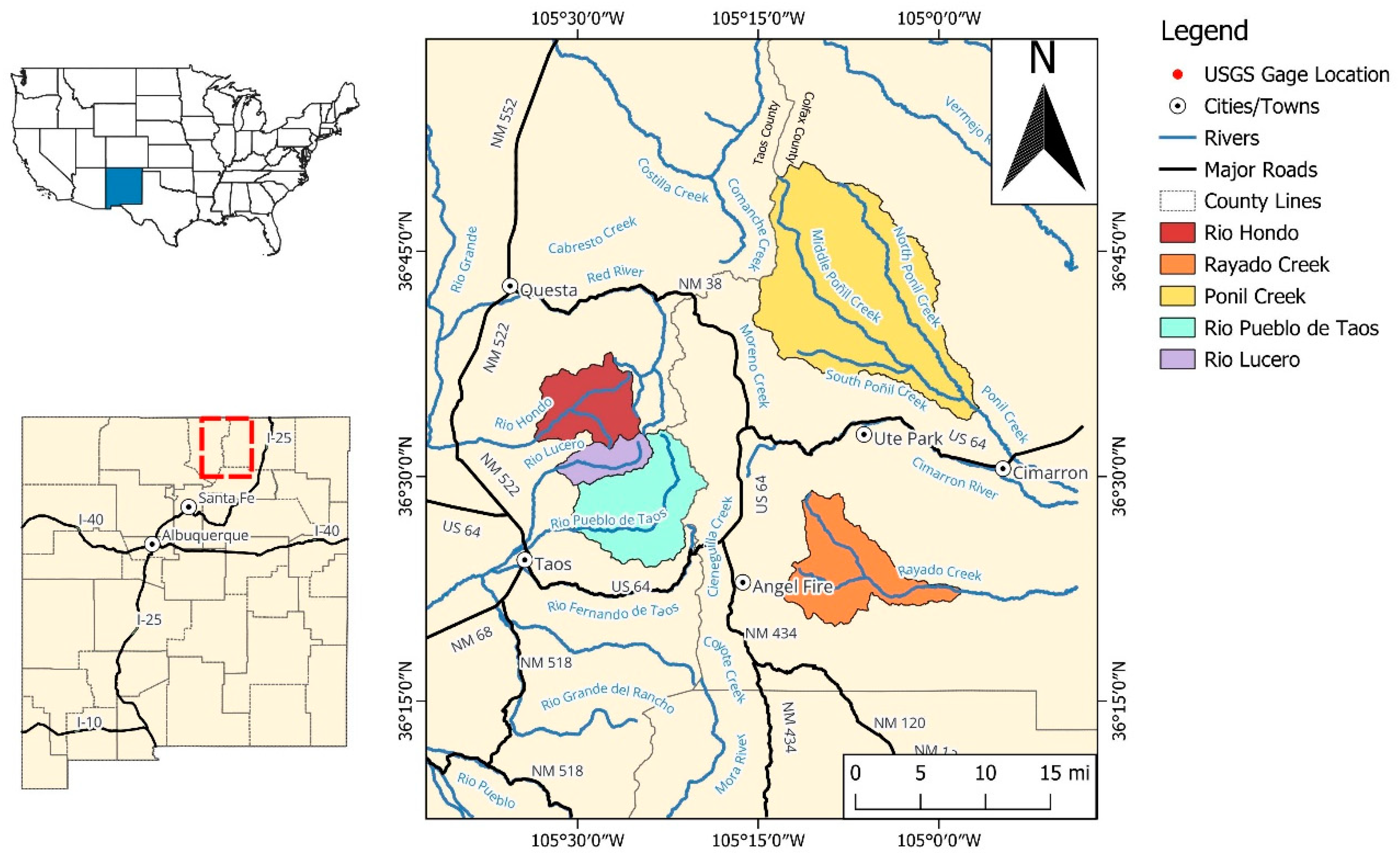
Figure 2.
Predictive Uncertainty Analysis Results for the Rio Hondo for high flow conditions of 50 to 450 CFS (a) and low flow conditions of 0 to50 CFS (b), and a quantile–quantile (QQ) probability plot (c).
Figure 2.
Predictive Uncertainty Analysis Results for the Rio Hondo for high flow conditions of 50 to 450 CFS (a) and low flow conditions of 0 to50 CFS (b), and a quantile–quantile (QQ) probability plot (c).
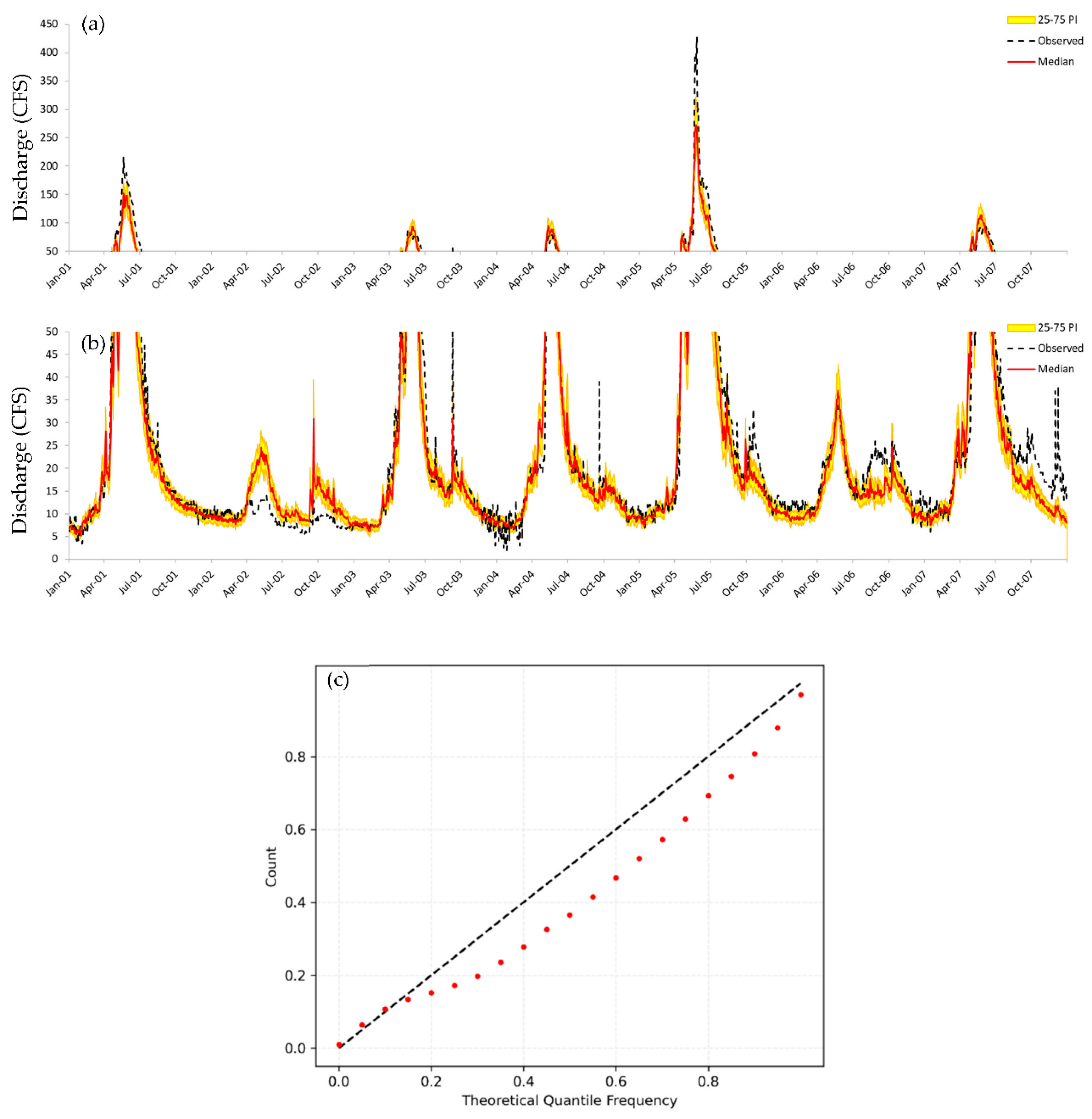
Figure 3.
Taos County (NM) Percent Area in U.S. Drought Monitor Categories.
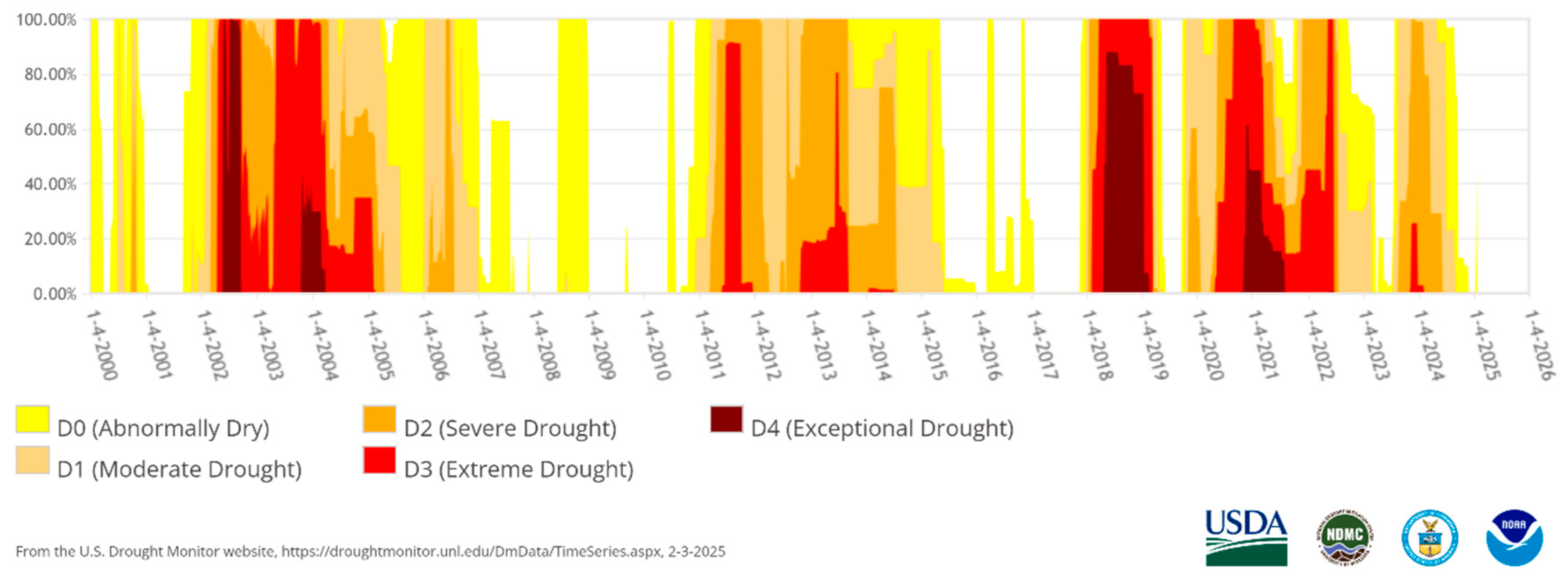
Figure 4.
Colfax County (NM) Percent Area in U.S. Drought Monitor Categories.
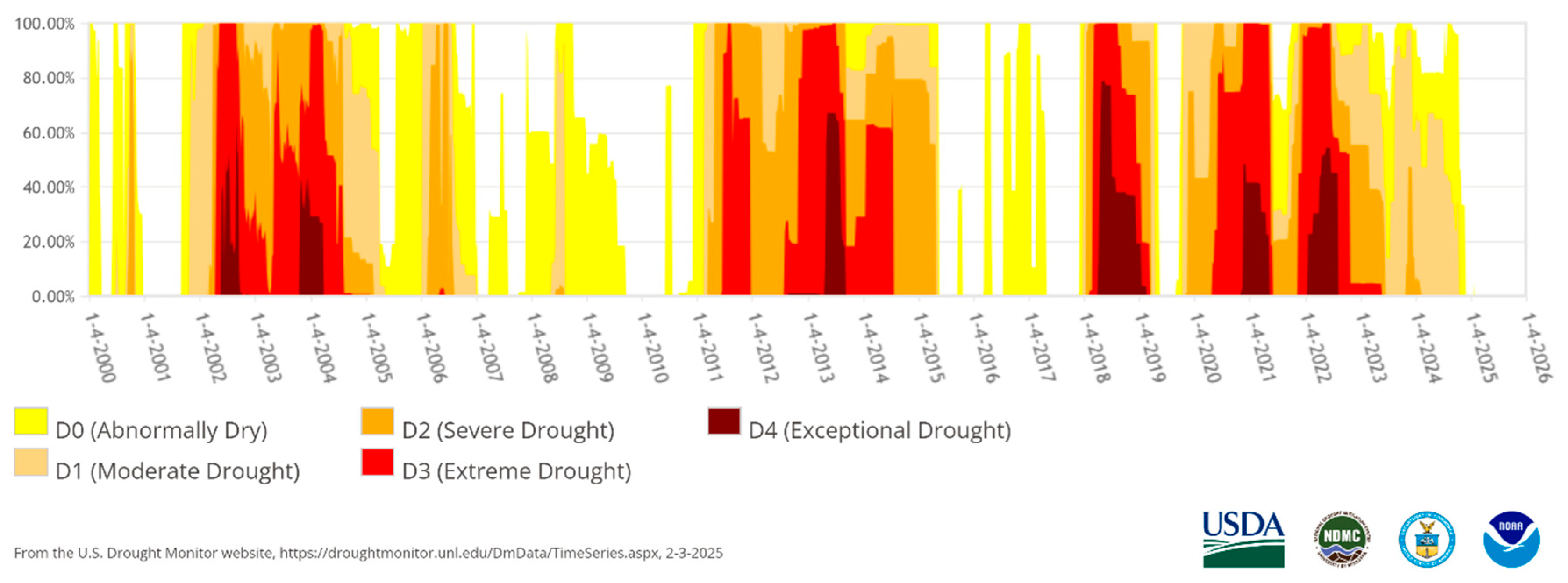
Figure 5.
High mountain streamflow generation from (a) hillslope response and runoff and (b) groundwater from recharge at higher elevations as described by Frisbee et al. (2011) adapted for the Rio Hondo basin. 3D orientation is depicted in the bottom left.
Figure 5.
High mountain streamflow generation from (a) hillslope response and runoff and (b) groundwater from recharge at higher elevations as described by Frisbee et al. (2011) adapted for the Rio Hondo basin. 3D orientation is depicted in the bottom left.
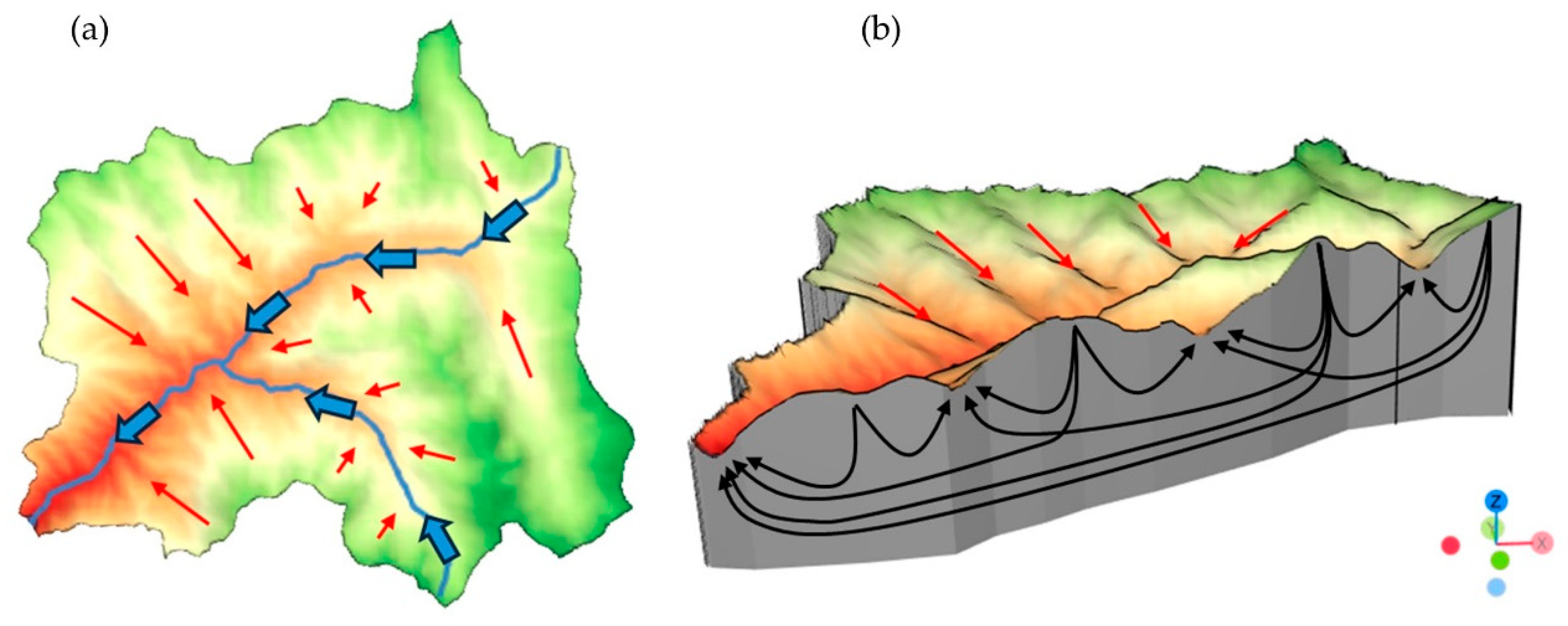
Figure 6.
Normalized cell state activations with strong correlation plotted against Normalized HEC-HMS derived depicting (a) strong positive correlation with Baseflow 1, and (b) strong positive corellation with baseflow 2.
Figure 6.
Normalized cell state activations with strong correlation plotted against Normalized HEC-HMS derived depicting (a) strong positive correlation with Baseflow 1, and (b) strong positive corellation with baseflow 2.
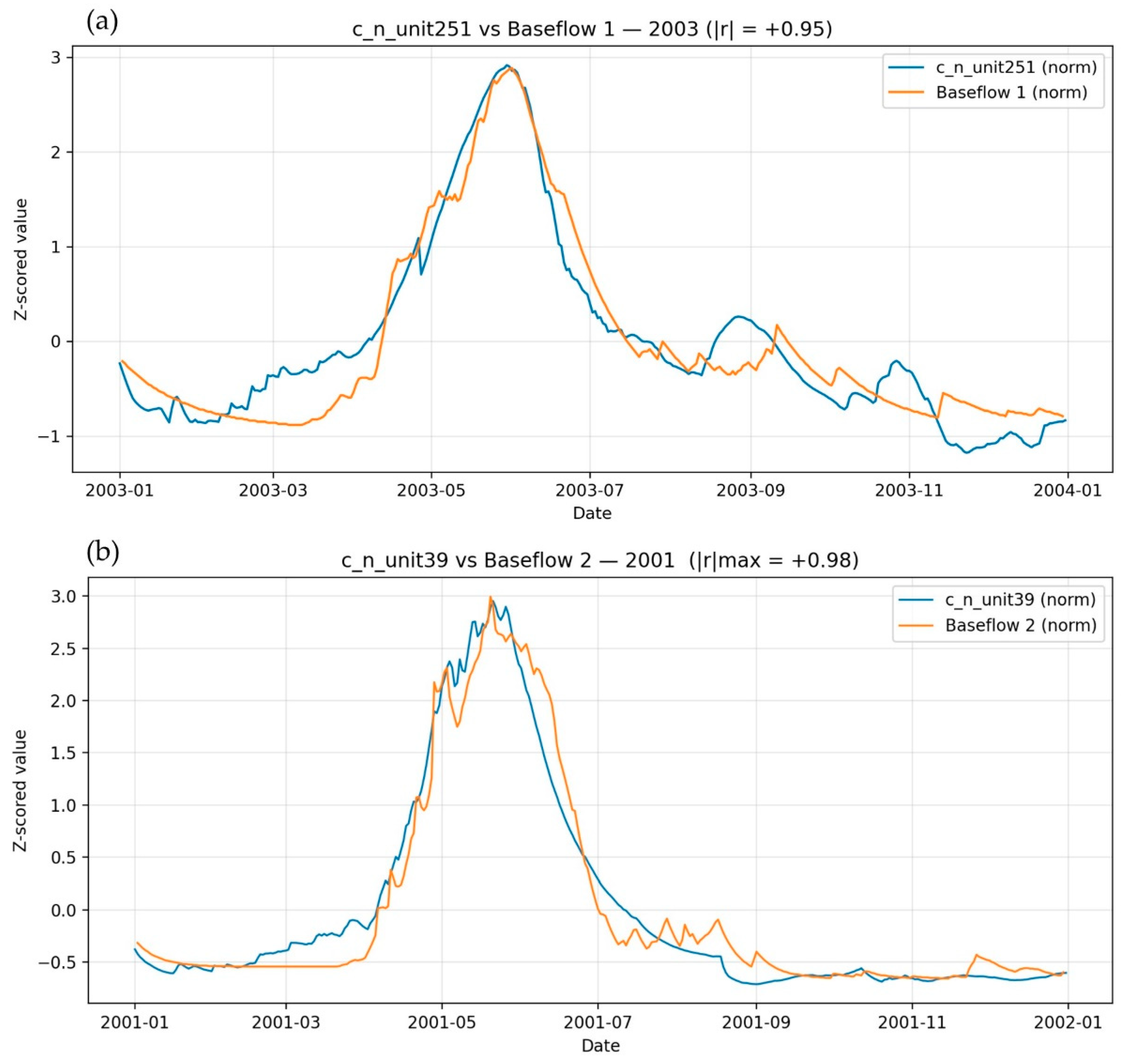
Figure 7.
LSTM Unit Correlation by Groundwater Source and Memory Type.
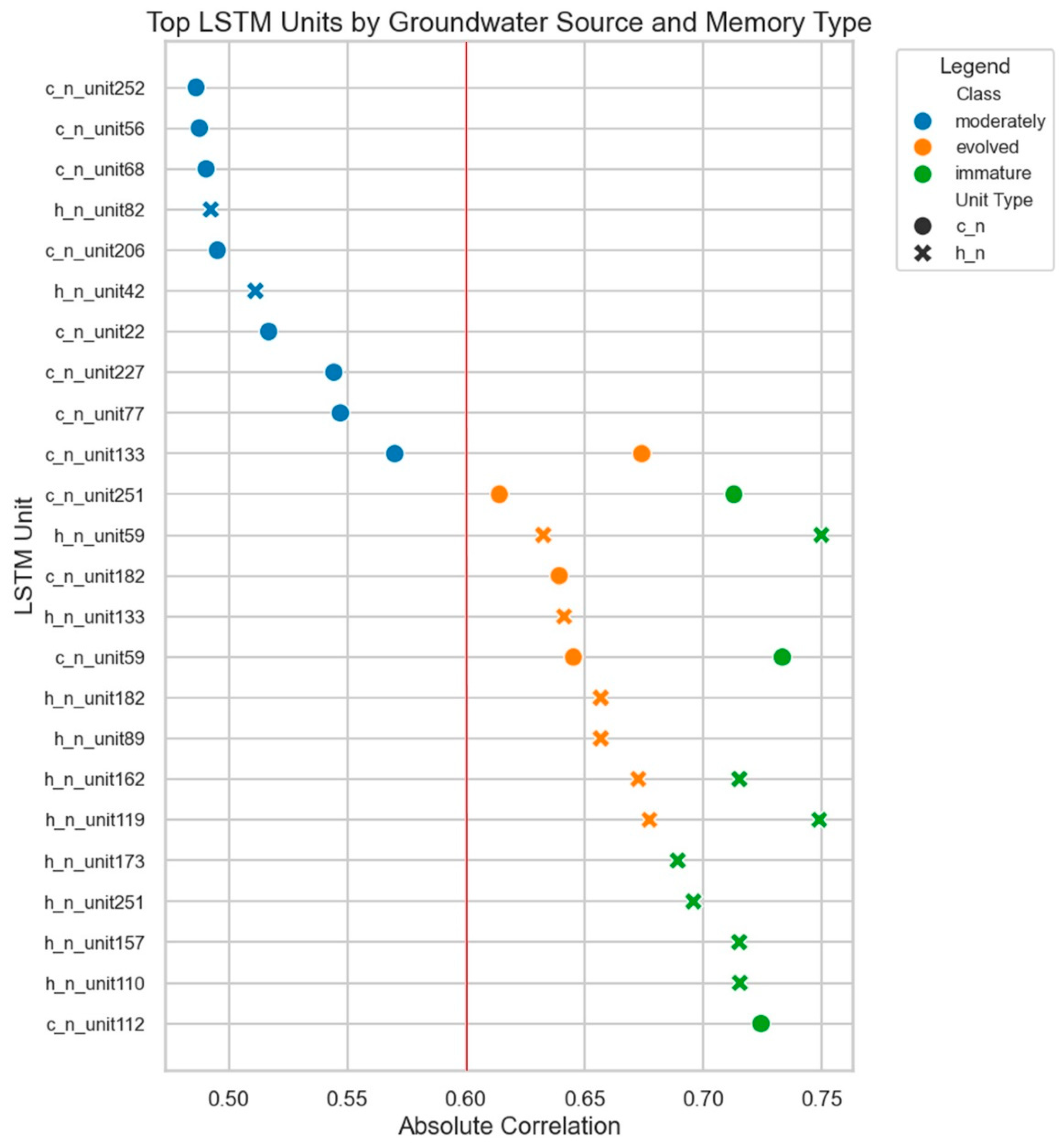
Figure 8.
Cluster Analysis Based on Correlation Patterns.
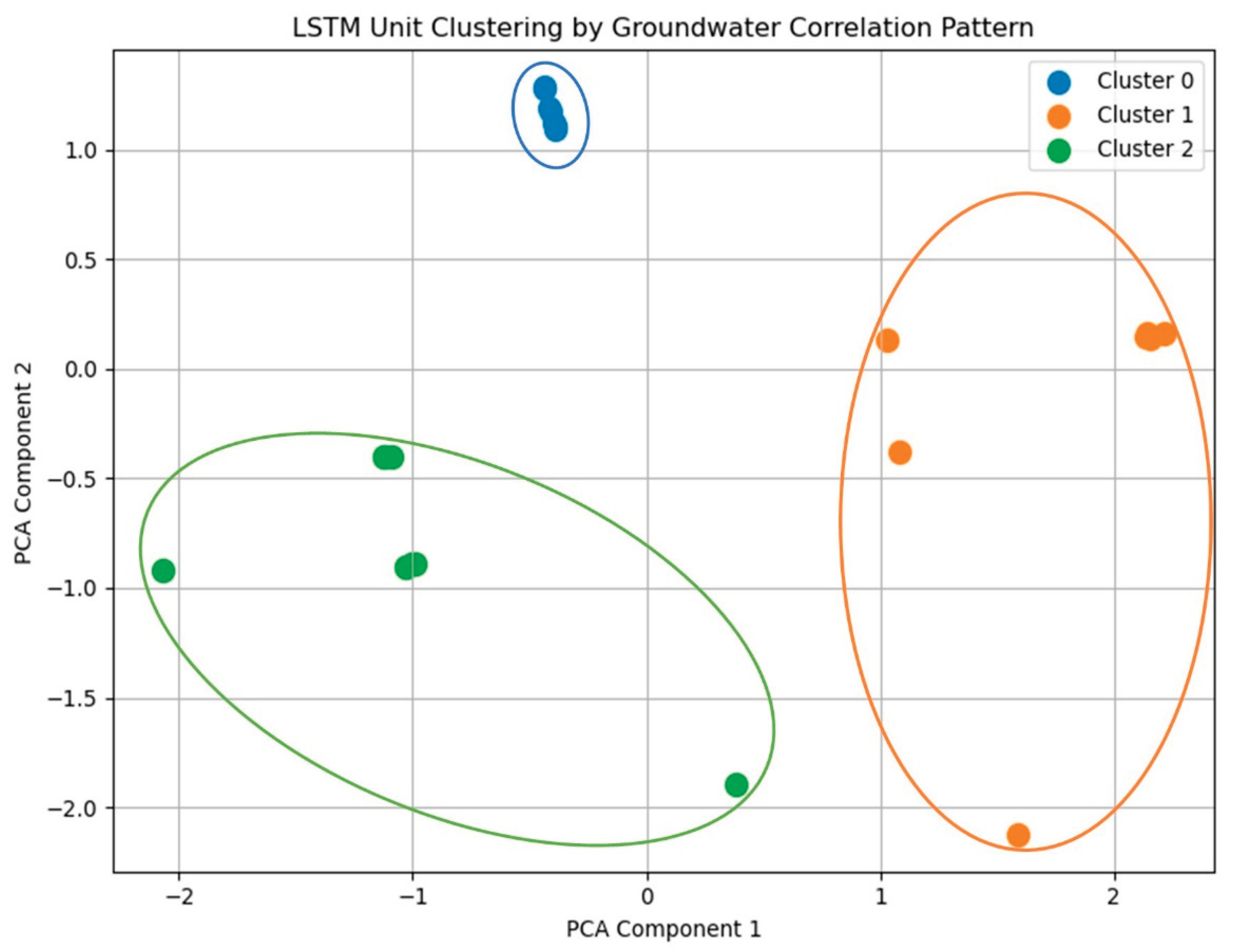

Table 1.
Basin Characteristics.
| Basin | Latitude (Degrees) |
Longitude (Degrees) |
Mean Basin Slope | Drainage Area (mi2) | Mean Elevation (ft, amsl*) | Outlet Elevation (ft, amsl*) |
|---|---|---|---|---|---|---|
| Hondo | 36.54 | -105.56 | 0.52 | 37.20 | 10390 | 7659 |
| Lucero | 36.51 | -105.53 | 0.51 | 16.90 | 10726 | 8071 |
| Taos | 36.44 | -105.50 | 0.38 | 63.10 | 9607 | 7400 |
| Rayado | 36.37 | -104.97 | 0.23 | 61.20 | 9502 | 6746 |
| Ponil | 36.57 | -104.95 | 0.25 | 186.00 | 8589 | 6640 |
* above mean sea level.
Table 2.
Model Hyperparameters.
| Sequence Length | Dropout | Learning Rate | Hidden Layer Embedding | Batch Size | Initial Learning Rate | Learning Rate at Epoch 10 | Learning Rate at Epoch 20 | Learning Rate at Epoch 40 |
|---|---|---|---|---|---|---|---|---|
| 365 | 0.2 | 0.003 | 128-64-128 | 64 | 5.00E-04 | 3.00E-04 | 1.00E-04 | 5.00E-05 |
Table 3.
Summary of Model Variables.
| Variable | Unit | Data Source |
|---|---|---|
| Precipitation | mm/day | Daymet |
| Daylight Seconds | Sec | Daymet |
| Shortwave Radiation | W/m 2 | Daymet |
| Max Temperature | oC | Daymet |
| Min Temperature | oC | Daymet |
| Vapor Pressure | Pa | Daymet |
| Snow Water Equivalent | Inches | Daymet |
| Observed flow | CFS | USGS |
| Latitude | Degrees | USGS |
| Longitude | Degrees | USGS |
| Elevation | Feet above Sea Level | USGS |
| Drainage Area | Acres | USGS |
| Surface Characteristics | NA | USGS |
| Accumulated Snow Water Equivalent | mm | DHWBDP |
| Actual Evapotranspiration | mm | DHWBDP |
| Potential Evapotranspiration | mm | DHWBDP |
| Deficit | mm | DHWBDP |
| Rain | mm | DHWBDP |
| Runoff | mm | DHWBDP |
| Soilwater | mm | DHWBDP |
Table 4.
Optimized HEC-HMS Parameters for Snowmelt and GW contributions.
| Model year | 2000 | 2001 | 2002 | 2003 | 2004 |
|---|---|---|---|---|---|
| Base Temperature | 45 | 40 | 33 | 39 | 44 |
| Snow vs Rain Temperature | 32 | 32 | 34 | 32 | 33 |
| Rain Rate Limit | 0.1 | 0.1 | 0.1 | 0.5 | 0.1 |
| Cold Limit | 0.02 | 0.01 | 0.08 | 0.02 | 0.02 |
| ATI Coefficient | 0.7 | 0.9 | 0.7 | 0.5 | 0.6 |
| GW-1 Baseflow Fraction | 0.04 | 0.06 | 0.01 | 0.06 | 0.05 |
| GW-2 Baseflow Fraction | 0.09 | 0.1 | 0.07 | 0.09 | 0.07 |
| GW-1 Routing Coefficient | 1050 | 200 | 2200 | 600 | 300 |
| GW-2 Routing Coefficient | 1500 | 1000 | 2400 | 1000 | 1600 |
Table 5.
Annual HEC-HMS calibration performance metrics.
| Water Year | Mean Flow (cfs) | Max Flow (cfs) | Volume (ac-ft) | NSE | RMSE/Stdev | PBIAS (%) | R² |
|---|---|---|---|---|---|---|---|
| 2000 | 13.1 | 40 | 9,471 | 0.81 | 0.44 | -1.25 | 0.81 |
| 2001 | 36.04 | 216 | 25,933 | 0.92 | 0.27 | 0.72 | 0.93 |
| 2002 | 9.15 | 16 | 6,222 | 0.39 | 0.80 | -3.29 | 0.51 |
| 2003 | 23.23 | 89 | 16,757 | 0.92 | 0.28 | -1.09 | 0.93 |
| 2004 | 20.05 | 79 | 14,491 | 0.9 | 0.32 | -0.21 | 0.9 |
Table 6.
Validation Metrics.
| Basin | NSE | KGE | RMSE (CFS) |
α-NSE | ß-NSE | ß-KGE | Pearson-r | FMS (%) |
FLV (%) |
|---|---|---|---|---|---|---|---|---|---|
| Hondo | 0.88 | 0.75 | 12.69 | 0.78 | -0.07 | 0.90 | 0.96 | -3.36 | 67.24 |
| Lucero | 0.90 | 0.79 | 6.75 | 0.81 | -0.06 | 0.93 | 0.96 | -15.52 | 26.67 |
| Taos | 0.85 | 0.77 | 12.67 | 0.78 | -0.02 | 0.97 | 0.94 | -13.40 | 50.87 |
| Rayado | 0.85 | 0.79 | 6.14 | 0.84 | -0.07 | 0.89 | 0.93 | -35.88 | 33.75 |
| Ponil | 0.49 | 0.37 | 21.40 | 0.57 | -0.16 | 0.63 | 0.74 | -30.72 | 58.05 |
Table 7.
Pre Drought Conditions (2000-2001).
| Basin | NSE | KGE | RMSE (CFS) |
α-NSE | ß-NSE | ß-KGE | Pearson-r | FMS (%) |
FLV (%) |
|---|---|---|---|---|---|---|---|---|---|
| Hondo | 0.87 | 0.64 | 16.42 | 0.71 | -0.16 | 0.79 | 0.99 | -10.27 | 52.29 |
| Lucero | 0.89 | 0.68 | 8.83 | 0.73 | -0.13 | 0.83 | 0.99 | -6.82 | 41.24 |
| Taos | 0.94 | 0.78 | 9.01 | 0.79 | -0.06 | 0.91 | 0.99 | -10.11 | 22.97 |
| Rayado | 0.95 | 0.92 | 2.29 | 0.93 | 0.01 | 1.01 | 0.98 | -20.00 | 78.48 |
| Ponil | 0.83 | 0.75 | 4.11 | 1.20 | 0.09 | 1.14 | 0.95 | -35.18 | -105.77 |
Table 8.
Drought Conditions (2002-2004).
| Basin | NSE | KGE | RMSE (CFS) |
α-NSE | ß-NSE | ß-KGE | Pearson-r | FMS (%) |
FLV (%) |
|---|---|---|---|---|---|---|---|---|---|
| Hondo | 0.90 | 0.92 | 5.24 | 1.01 | 0.06 | 1.06 | 0.95 | 5.14 | 77.84 |
| Lucero | 0.90 | 0.81 | 4.13 | 0.81 | 0.04 | 1.04 | 0.96 | -20.96 | 18.82 |
| Taos | 0.66 | 0.65 | 8.55 | 1.24 | 0.18 | 1.23 | 0.90 | -14.31 | 58.65 |
| Rayado | 0.83 | 0.80 | 3.54 | 1.15 | 0.09 | 1.13 | 0.94 | -16.20 | 37.20 |
| Ponil | 0.35 | 0.20 | 25.22 | 0.41 | -0.13 | 0.58 | 0.65 | -55.17 | 60.64 |
Table 9.
Base Flow Indices for Drought Conditions and Pre Drought Conditions.
| Basin | Pre Drought BFI | Drought BFI | ||
|---|---|---|---|---|
| Observed | Simulated | Observed | Simulated | |
| Hondo | 0.32 | 0.36 | 0.56 | 0.56 |
| Lucero | 0.32 | 0.36 | 0.51 | 0.56 |
| Taos | 0.28 | 0.32 | 0.44 | 0.47 |
| Rayado | 0.36 | 0.39 | 0.45 | 0.47 |
| Ponil | 0.22 | 0.23 | 0.21 | 0.29 |
Disclaimer/Publisher’s Note: The statements, opinions and data contained in all publications are solely those of the individual author(s) and contributor(s) and not of MDPI and/or the editor(s). MDPI and/or the editor(s) disclaim responsibility for any injury to people or property resulting from any ideas, methods, instructions or products referred to in the content. |
© 2025 by the authors. Licensee MDPI, Basel, Switzerland. This article is an open access article distributed under the terms and conditions of the Creative Commons Attribution (CC BY) license (http://creativecommons.org/licenses/by/4.0/).
Copyright: This open access article is published under a Creative Commons CC BY 4.0 license, which permit the free download, distribution, and reuse, provided that the author and preprint are cited in any reuse.


