
Submitted:
14 July 2025
Posted:
15 July 2025
You are already at the latest version
Abstract
Mid–long term streamflow prediction (MLSP) plays a critical role in water resource planning amid growing hydroclimatic and anthropogenic uncertainties. Although AI-based models have demonstrated strong performance in MLSP, their capacity to quantify predictive uncertainty remains limited. To address this challenge, a DeepAR-based probabilistic modeling framework is developed, enabling direct estimation of streamflow distribution parameters and flexible selection of output distributions. The framework is applied to two case studies with distinct hydrological characteristics, where combinations of recurrent model structures (GRU and LSTM) and output distributions (Normal, Student’s t, and Gamma) are systematically evaluated. Results indicate that models employing the Gamma distribution consistently outperform those using Normal and Student’s t distributions. In the Upper Wudongde Reservoir area, the model using LSTM structure and Gamma distribution reduces RMSE from 1407.77 m³/s to 1016.54 m³/s. As the forecast horizon extends, the Gamma-based models demonstrate more reliable probabilistic predictions, reflected by sharper and better-calibrated prediction intervals. This is evidenced by substantially reduced CRPS values at the 18th forecast horizon (521.4 and 1746.6 m³/s), compared to Normal-based models (747.6 and 1877.5 m³/s). Although the improvements in predictive performance achieved by the proposed modeling framework vary depending on the RNN model architecture used and the specific application region, it generally delivers consistent enhancement in forecasting accuracy, thereby providing stronger support for practical applications.
Keywords:
mid-long term streamflow prediction
; probabilistic prediction
; DeepAR
; modeling framework
; Gamma distribution
1. Introduction
The combined impacts of climate change and human activities are profoundly altering the processes of runoff generation and confluence, resulting in increasing uncertainty in the evolution of water resources [1,2,3,4]. At the same time, socio-economic drivers such as population growth and urbanization are intensifying the demand for water supply [5,6,7,8]. Against this backdrop, mid-long term streamflow prediction (MLSP) has become increasingly vital for effective water resources management and integrated utilization, as it provides valuable insights into future runoff patterns [9,10,11,12,13,14]. Consequently, MLSP is attracting growing attention in both research and practical applications [11,12,13,14].
Many models have been developed and applied in MLSP to improve the predictive performance, and provide information for the comprehensive utilization of water resources [11,12,13,14,15,16,17]. These models can be broadly divided into physical-based models, which simulate the streamflow based on the runoff generation and confluence equations, and data-driven models, which directly simulate the relationship between streamflow and predictors including precipitation, temperature and other factors [13,14,18,19,20,21]. Along with the development of artificial intelligence (AI) methods, the AI-based data-driven models, including support vector regression (SVR), artificial neural network (ANN), gated recurrent unit neural network (GRU), long short-term memory network (LSTM) and so on, can obtain better predictive performance than traditional models and have become predominant in the MLSP [10,19,22,23,24,25,26]. For instance, many studies applied SVR models in MLSP and the results demonstrate that the SVR models can generate more accurate forecasts than linear models and ANN models [27,28,29,30,31]. Xie et al. (2024) compared five AI-based models and the results demonstrate that the LSTM model outperformed other models in forecasting monthly streamflow in 37 basins [14].
The proposed AI-based models in MLSP demonstrate significant improvements in predictive performance, but their limited capacity to characterize future water resource uncertainties constrains practical applications [32,33,34,35]. To overcome this issue, many post-processing methods are adopted to produce ensemble forecasting results capable of characterizing predictive uncertainties [34,35,36]. For example, Liang et al. (2018) proposes the hydrological uncertainty processor to post-process the deterministic outputs from the SVR model to quantify prediction uncertainties [33]. Mo et al. (2023) applies the generalized autoregressive conditional heteroskedasticity model to identify time-varying forecasting errors to improve the predictive performance [37].
Although the post-processing approach in MLSP demonstrates predictive capability, it exhibits two fundamental limitations: (1) inability to directly generate probability distributions, and (2) failure to preserve the inherent statistical characteristics of streamflow. To overcome these constraints in MLSP, this study adopts a DeepAR-based modeling framework. The DeepAR architecture exhibits two key capabilities: (1) direct prediction of the predictand's distribution parameters, and (2) flexible selection of probability distributions for the target variable [38,39]. Empirical validation across five time series datasets demonstrates its superior performance over other existing state-of-the-art methods. However, the DeepAR's robustness under heavy-tailed streamflow distributions requires further verification, and the selection criteria for appropriate probability distributions lack systematic guidance. Therefore, the objectives of this study are (1) to develop a DeepAR-based probabilistic forecasting framework for MLSP, (2) to validate modeling framework's applicability through implementation in two case studies, and (3) to systematically evaluate impacts of base model architecture and distribution type selection on predictive skill.
The remaining sections of this paper are organized as follows. The data, case studies and methods are introduced in section 2. The results will be demonstrated in section 3 and discussed in section 4. Finally, the main conclusions will be summarized in section 5.
2. Materials and Methods
2.1. DeepAR Model
DeepAR is a probabilistic forecasting framework developed by Amazon Research, which combines recurrent neural networks (RNNs) with parametric probability distributions to generate time-series predictions [38]. Unlike traditional point-forecasting models, DeepAR directly outputs the parameters of user-specified distributions (e.g., Gaussian for real-valued data, Negative Binomial for positive count data, Beta for data in the unit interval), enabling native uncertainty quantification.
Let denotes the streamflow value at time t, and represents the vector of predictor variables at time t. The DeepAR model estimates the conditional distribution of future streamflow values:
where is the forecast initialization time, is the context length and is the prediction length.
For a trained DeepAR model, the distribution parameters at time t are computed as a function of the hidden state and model parameters :
where is a function used to map the hidden state to distribution parameters, and the hidden state evolves recursively via:
where is a nonlinear transition function implemented as a multi-layer RNN (LSTM or GRU) parametrized by , and is the hidden state from the previous time step.
Then the simulated or forecasted streamflow value at time t can be sampled by:
2.1.1. Training
Given a streamflow time series and associated predictor variables , the DeepAR model parameters , including the parameters of both the and , can be learned by maximizing the log-likelihood as below:
2.1.2. Prediction
Given an observed streamflow sequence and corresponding predictor variables , the trained DeepAR model generates probabilistic forecasts for future streamflow values through the following procedure:
1) The hidden state is obtained by recursively processing the historical streamflow and predictors through the RNN transition function in Equation (3);
2) Initial conditions are set as and ;
3) For each subsequent time step to , the hidden state is updated using , the forecast is sampled from , and
4) Step 3) is repeated N times to produce an ensemble forecasts , providing a Monte Carlo approximation of the predictive distribution.
2.1.3. Likelihood Model
The likelihood , which defines the target distribution, must be carefully selected to match the statistical characteristics of predictand. While Salinas et al. (2020) recommended Gaussian distributions for real-valued data and Negative Binomial distributions for positive count data, these choices prove suboptimal for streamflow forecasting due to: 1) heavy-tailed characteristics of streamflow, and 2) the strictly positive nature of streamflow values. Therefore, to better characterize the statistical properties of streamflow, this study employs Student's t-distribution which is suitable for extreme events, Gamma distribution which is suitable for skewed streamflow, and conventional Gaussian distribution.
For Student's t-distribution, the likelihood and function are as below:
where the softplus activation function is applied to enforce positivity constraints on the distribution parameters.
For Gamma distribution, the likelihood and function are as below:
2.2. DeepAR-Based Modeling Framework
This study develops a DeepAR-based probabilistic forecasting framework for MLSP (Figure 1), which consists of four main steps: (1) data preparing, involving data collection and optimal distribution selection, (2) data splitting, which spites data into training, validation and test datasets, (3) model calibration, involving model training and selection, and (4) model evaluation, involving model performance assessment [40,41].
2.2.1. Data Preparing
Data preparing and analysis are proposed to collect streamflow and corresponding predictors (precipitation), and select optimal distribution for the streamflow. To select the most appropriate distribution from these candidates, both the Akaike Information Criterion (AIC) and Bayesian Information Criterion (BIC) are employed to evaluate the goodness-of-fit between the observed data and theoretical distributions. Then the optimal distribution is selected by minimizing both AIC and BIC values, which are computed as:
where Li is the maximized likelihood value, k denoted parameters number, and n is length of streamflow time series.
2.2.2. Data Splitting
Data splitting is an important step in data-driven modeling process, through which the available data is divided into training, validation and test datasets [40,41,42]. In this study, the data after a specific time point is first separated as the test set to ensure no overlap between the test set data and other data. Subsequently, the remaining data is randomly shuffled and split into training and validation datasets in an specific ratio.
2.2.3. Model Calibration
Model calibration is used to optimize model architecture and parameters in order that the model can represent the underlying relationships between predictors and predictand. First, the optimal streamflow distribution obtained by minimizing the AIC/BIC metrics is adopted to define the model architecture (i.e. model’s output distribution type). Then, multiple model variants are generated by varying input conditions and parameters are optimized using training dataset by the ADAM optimizer [43]. Finally, the model variants are used in validation dataset and compared to select the best model in terms of their predictive performance.
2.2.4. Model Evaluation
Model evaluation is used to assess the predictive performance of the selected model over an independent dataset (i.e. test dataset) [44]. The deterministic and probabilistic predictions are generated and two metrics are proposed to evaluate the predictive performance: 1) root mean square error (RMSE), quantifying the accuracy of ensemble mean predictions against observations; and 2) continuous ranked probability score (CRPS), which measures the overall probabilistic predictive performance [45,46]. These two metrics can be calculated according to the following equations:
where n is the sample size in test dataset, i is the sample index, is the observed streamflow, is the ensemble mean prediction, is the cumulative distribution function (CDF) of the probabilistic forecast.
2.3. Case Study and Data
The performance of the DeepAR-based modeling framework is examined in two basins upstream of the Wudongde (WDDR) and Sanxia (SXR) reservoirs, as illustrated in Figure 2. The available data and statistical characteristics for the two basins is presented in Table 1, including ten-day naturalized streamflow and areal mean precipitation records spanning January 1980 to September 2022. To ensure data compatibility with neural network requirements, all variables are first normalized before model processing, and then inversely transformed to their original scales.
2.4. Experiment Setup
Following the DeepAR-based modeling framework, three candidate distribution types—Gaussian, Gamma, Student’s t-distribution—are provided to account for streamflow characteristics during the data preparing stage. Then, the data after January 2017 is separated as the test dataset, while the other data is randomly split into training and validation datasets at an 8:2 ratio.
During the model calibration phase, different models for predicting streamflow in the next 18 ten-day periods, are trained based on varying input conditions that incorporate combinations of three precipitation input scenarios (temporal lags: [0], [0,1] or [0,1,2]) and two streamflow input scenarios (temporal lags: [1], [1,2]). The optimal input combination is then selected based on comparative evaluation of all model variants' predictive performance (i.e. RMSE) on the validation dataset.
After data preparing and model calibration, the final model combining the optimal input configuration and the probability distribution output is established and applied to produce deterministic predictions and probabilistic predictions with 100 members in this study. In order to evaluate the impact of output distribution and RNN structure, alternative models with different probability distribution outputs and different RNN structures (LSTM and GRU), named GRU-N, GRU-S, GRU-G, LSTM-N, LSTM-S, LSTM-G, are established and compared in terms of their predictive performance on the testing dataset. In the “GRU-N” naming structure, the former denotes the RNN structure (including GRU and LSTM), while the latter denotes the model output distribution (including normal distribution N, Student's t-distribution S, and Gamma distribution G).
3. Results
Following the modeling framework, the results are presented in three sections: optimal probability distribution selection (Section 3.1), input configuration optimization (Section 3.2), and testing performance evaluation (Section 3.3).
3.1. Optimal Probability Distribution Selection
The distribution fitting results for both study areas are presented in Figure 3, while the corresponding AIC and BIC values are listed in Table 2. The results reveals that the Gamma distribution provides superior statistical performance compared to Normal and Student's t-distributions. For the Upper WDDR area, the Gamma distribution achieves the lowest AIC (27321.09) and BIC (27337.03) values, substantially outperforming the Normal distribution (AIC: 28574.36, BIC: 28584.99) and Student's t-distribution (AIC: 28455.62, BIC: 28471.57). Similarly, in the Upper SXR area, the Gamma distribution exhibits superior performance with AIC (30848.71) and BIC (30864.66) values considerably lower than the alternative distributions. The probability density plots also illustrate that the Gamma distribution more accurately captures the right-skewed characteristics and tail behavior of the streamflow data in both study areas.
3.2. Input Configuration Optimization
The comparative analysis of different input configurations reveals consistent performance patterns across both study areas. For the Upper WDDR area, the precipitation input scenario with temporal lags [0,1,2] achieves the lowest RMSE (1199.21 m3/s), indicating superior predictive accuracy when incorporating precipitation data from the current time step and two previous time steps. In contrast, the precipitation-only scenario with no temporal lag [0] shows the poorest performance with the highest RMSE (1277.07 m3/s). Similarly, in the Upper SXR area, the [0,1,2] precipitation configuration demonstrates optimal performance with an RMSE value of 3481.18 m3/s, while the [0] configuration shows the highest RMSE (3634.35 m3/s). The performance gradient follows a consistent pattern across both areas, where increased temporal lag information progressively improves model accuracy.
Regarding streamflow input configurations, the comparison between temporal lags [1] and [1,2] shows that incorporating additional historical streamflow information ([1,2]) yields only marginal improvements, with RMSE decreasing modestly from 1245.33 to 1230.19 m3/s in the Upper WDDR area and from 3577.72 to 3577.31 m3/s in the Upper SXR area. This suggests that the contribution of additional streamflow lag information is relatively limited compared to the substantial performance gains observed with precipitation temporal lags.
3.3. Testing Performance Evaluation
The predictive performance metrics of the six models (i.e. GRU-N, GRU-S, GRU-G, LSTM-N, LSTM-S, LSTM-G) are presented in Table 4. Models with Gamma distribution output achieve the best performance in both study areas and evaluation metrics. In the Upper WDDR area, LSTM-G demonstrates the lowest RMSE (1016.54 m3/s) and CRPS (473.26 m3/s), followed by GRU-G with RMSE of 1098.98 m3/s and CRPS of 517.54 m3/s. For the Upper SXR area, LSTM-G also shows superior performance with RMSE of 4047.15 m3/s and CRPS of 1717.93 m3/s. The differences between GRU and LSTM architectures are relatively small and show no consistent patterns. In Upper WDDR, LSTM-G slightly outperforms GRU-G, while in Upper SXR, the differences are marginal. This suggests that RNN architecture choice has minimal impact compared to output distribution selection.
4. Discussion
The predictive performance of the six models (i.e. GRU-N, GRU-S, GRU-G, LSTM-N, LSTM-S, LSTM-G) is discussed in this section. First, Section 4.1 discusses the deterministic prediction performance (i.e., RMSE) of models with different distribution outputs and different RNN structures across various forecast horizons. Then, Section 4.2 provides a comparative analysis of their probabilistic prediction performance (i.e., CRPS). Finally, Section 4.3 demonstrates the overall predictive performance of the models across different forecast horizons.
4.1. Deterministic Prediction Performance of Different Models
The deterministic predictive performance (i.e., RMSE) of six models (i.e., GRU-N, GRU-S, GRU-G, LSTM-N, LSTM-S, LSTM-G) across 18 forecast horizons (10-day periods) for two study areas is presented in Table 5 and Figure 4. It is evident that the forecasting accuracy is generally observed to decline as the forecast horizon increases, regardless of model architecture or output distribution. Among the three distributions, the Gamma distribution consistently results in lower RMSE values, particularly at longer lead times. This suggests a better capacity of the Gamma-based models to capture the positively skewed or heteroscedastic characteristics often found in hydrological data. In the Upper WDDR area, the LSTM-G model achieves the lowest RMSE across most forecast horizons, with values ranging from 859.8 m3/s at the 1st forecast period to 1096.7 m3/s at the 18th. A similar pattern is observed in the Upper SXR area, where LSTM-G yields the minimum RMSE of 3687.7 m3/s at the 1st period and 3998.1 m3/s at the 18th.
Differences between LSTM and GRU structures are also observed but are found to be less consistent and less influential than those resulting from output distribution selection. In the Upper WDDR area, GRU-N and GRU-S outperform their LSTM counterparts, while the advantage shifts to LSTM only when the Gamma distribution is employed. In the Upper SXR area, the superiority of LSTM-G is observed only at shorter forecast horizons, with GRU-G performing better as the forecast horizon increases. Across all configurations, no consistent advantage is associated with either architecture, suggesting that model structure plays a secondary role relative to the output distribution in determining predictive performance.
Notably, the magnitude of performance gains brought by the Gamma distribution varies across regions. In the Upper WDDR area, the use of Gamma distribution yields substantial improvements compared to Normal and Student’s t assumptions, particularly when paired with LSTM. In contrast, in the Upper SXR area, although Gamma-based models still outperform others, the improvement is relatively marginal. For instance, the reduction in RMSE from LSTM-N to LSTM-G at the 18th horizon is only modest (from 4203.0 m3/s to 4070.5 m3/s), whereas the gain is more pronounced in the Upper WDDR region (from 1559.5 m3/s to 1096.7 m3/s). These findings demonstrate that the benefit of applying flexible, non-Gaussian output distributions such as Gamma is region-dependent and may vary with underlying hydrological complexity or data characteristics.
In summary, the results highlight the critical role of output distribution in deterministic streamflow forecasting, with the Gamma distribution consistently offering performance benefits, though to varying extents across regions. While model structure has some impact, it exerts less influence than distributional assumptions.
4.2. Probabilistic Prediction Performance of Different Models
The probabilistic predictive performance (i.e., CRPS) of six models (i.e., GRU-N, GRU-S, GRU-G, LSTM-N, LSTM-S, LSTM-G) across 18 forecast horizons (10-day periods) for two study areas is presented in Table 6 and Figure 5. Similar to the deterministic results, probabilistic forecast accuracy generally declines with increasing lead time, as reflected by rising CRPS values across all model configurations. Among the output distributions, the Gamma distribution again provides the most substantial improvements in forecast skill. This consistency between deterministic and probabilistic evaluations reinforces the robustness of the Gamma assumption in capturing the inherent characteristics of streamflow data. In the Upper WDDR area, LSTM-G yields the lowest CRPS across nearly all horizons, ranging from 340.4 m3/s at the 1st period to 521.4 m3/s at the 18th. In the Upper SXR area, LSTM-G performs best during the first three horizons, while GRU-G shows superior accuracy at longer horizons. This pattern echoes deterministic results, where GRU-G also performed better in long-term forecasting under complex conditions.
Compared to output distribution selection, differences due to model structure are less consistent and generally less influential. While LSTM tends to perform better in the Upper WDDR area, GRU offers competitive or better results in the Upper SXR region when combined with the Gamma distribution.
Regional differences are again observed, with CRPS values in the Upper SXR region consistently higher than those in the Upper WDDR area, reflecting greater predictive uncertainty. However, the relative benefit of using the Gamma distribution persists in both regions, though with different magnitudes. For instance, at the 18th horizon, the CRPS reduction from GRU-N to GRU-G is more substantial in the Upper WDDR area (from 705.2 m3/s to 572.2 m3/s) than in the Upper SXR area (from 1843.3 m3/s to 1699.6 m3/s), consistent with patterns seen in deterministic forecasts.
In summary, probabilistic forecasting results confirm key findings from deterministic evaluations—particularly the consistent advantage of using the Gamma distribution across regions and horizons. However, nuanced differences are observed in the relative contributions of model structure, especially under probabilistic metrics. These findings suggest that while distributional assumptions remain the most critical component for improving streamflow forecast quality, model structure and regional hydrological characteristics jointly shape both deterministic and probabilistic forecasting performance.
4.3. Overall Predictive Performance
The predicted and observed streamflow at the 1st forecast horizon are shown in Figure 6. It is evident that all models produce narrow prediction intervals that closely follow the observations during non-flood seasons, when streamflow is low and uncertainty is limited. In contrast, flood seasons are characterized by increased variability, leading to wider forecast intervals and larger deviations, particularly around peak flows. The choice of output distribution also significantly affects forecast reliability: models using the Normal distribution often generate overly wide intervals due to their poor fit to the skewed nature of streamflow, whereas Gamma-based models produce tighter and more stable intervals. While Gamma-based models generally provide better predictions in most cases, their advantage may not hold in every situation—for example, the GRU-G model perform worst in the Upper WDDR region. Nonetheless, their ability to constrain uncertainty remains evident, and such model-specific variability also underscores the importance of model fusion strategies for improving forecast robustness under diverse application scenarios [20,47,48,49,50].
The predicted and observed streamflow across 18 forecast periods for models using Gamma distribution in both the Upper WDDR and Upper SXR regions are presented in Figure 7. As the forecast horizon increases, streamflow uncertainty becomes more pronounced, and the width of the predictive intervals correspondingly expands. This widening of intervals effectively reflects the growing uncertainty associated with longer lead times, particularly during high-flow periods. The use of the Gamma distribution enables the models to better capture the skewed nature of streamflow, resulting in predictive intervals that not only reflect the asymmetry of the data but also reliably encompass the observed hydrographs across seasons and forecast periods. This demonstrates the capability of using suitable output distribution to improve both the reliability and calibration in probabilistic streamflow prediction.
5. Conclusions
In this study, a DeepAR-based modeling framework is developed to generate probabilistic streamflow forecasts by integrating distribution selection with the DeepAR model. The framework is applied to two case studies to evaluate both deterministic and probabilistic forecasting performance. The influence of model structure and output distribution choice on prediction accuracy is also examined. The main conclusions are as follows.
The proposed DeepAR-based modeling framework effectively identifies the most appropriate output distribution and input configuration, leading to superior deterministic and probabilistic forecasting performance in both case studies. By integrating distribution selection and input optimization, the framework ensures that the final models are well-calibrated to the characteristics of local streamflow dynamics.
Multiple factors influence predictive performance, among which the selection of output distribution has the most significant impact. Meanwhile, differences between RNN model structures (i.e., GRU vs. LSTM) are relatively minor and less consistent. Additionally, regional differences in forecasting performance suggest that the effectiveness of a given model configuration is influenced by underlying hydrological conditions.
As forecast lead time increases and during flood seasons, streamflow uncertainty grows substantially. The developed probabilistic forecasting framework is capable of capturing this variation in uncertainty, and models using the Gamma distribution demonstrate superior performance by better representing the skewed nature of streamflow. This contributes to more reliable and better-calibrated forecasts across both typical and high-variability conditions.
Given that different models exhibit varying performance under different scenarios, future work could explore model fusion approaches to leverage complementary model strengths and enhance forecast robustness. Moreover, the framework’s generalizability could be further validated by testing a wider range of output distributions—tailored to characteristics of daily or annual streamflow and other hydro-meteorological variables—thereby expanding its applicability across diverse forecasting contexts.
Author Contributions
Conceptualization, S.X. and J.W.; methodology, S.X.; software, S.X. and K.S.; validation, S.X., D.W. and B.J.; formal analysis, S.X. and C.Y; investigation, D.W. and C.Y; resources, S.X. and K.S; data curation, J.W. and B.J.; writing—original draft preparation, S.X., J.W. and B.J.; writing—review and editing, D.W.; visualization, S.X. and C.Y; supervision, D.W.; project administration, S.X.; funding acquisition, D.W. All authors have read and agreed to the published version of the manuscript.
Funding
This research was funded by The National Key Research and Development Programof China (grant number: 2023YFC3206002), the Natural Science Foundation of Hubei Province (grant number: 2023AFB039, 2022CFD027), the National Natural Science Foundation of China (grant number: U2340211), the Key Project of Chinese Water Resources Ministry (grant number: SKS-2022120), and China Yangtze Power Co.,Ltd (contract no.Z242302057 and project no.2423020055). Shuai Xie is supported by a program of China Scholarship Council (No.202303340001) during his visit to the University of Regina, where the research is conducted.
Data Availability Statement
The raw data supporting the conclusions of this article will be made available by the authors on request.
Acknowledgments
Various Python open-source frameworks were used in this study. We would like to express our gratitude to all contributors. We would also like to give special thanks to the anonymous reviewers and editors for their constructive comments.
Conflicts of Interest
The authors declare no conflicts of interest.
Abbreviations
The following abbreviations are used in this manuscript:
| MLSP | mid–long term streamflow prediction |
| AI | artificial intelligence |
| SVR | support vector regression |
| ANN | artificial neural network |
| LSTM | long short-term memory network |
| GRU | gated recurrent unit neural network |
| RNN | recurrent neural network |
| WDDR | Wudongde Reservoir |
| SXR | Sanxia Reservoir |
| RMSE | root mean square error |
| CRPS | continuous ranked probability score |
References
- Nguyen, Q.H. and V. N. Tran, Temporal Changes in Water and Sediment Discharges: Impacts of Climate Change and Human Activities in the Red River Basin (1958–2021) with Projections up to 2100. Water 2024, 16, 1155. [Google Scholar]
- Jia, L. , et al. , Sensitivity of Runoff to Climatic Factors and the Attribution of Runoff Variation in the Upper Shule River, North-West China. Water 2024, 16, 1272. [Google Scholar]
- Xu, H. , et al., Assessment of climate change impact and difference on the river runoff in four basins in China under 1.5 and 2.0∘ C global warming. Hydrology & Earth System Sciences, 2019. 23(10).
- Zou, L. and T. Zhou, Near future (2016-40) summer precipitation changes over China as projected by a regional climate model (RCM) under the RCP8. 5 emissions scenario: Comparison between RCM downscaling and the driving GCM. Advances in Atmospheric Sciences 2013, 30, 806–818. [Google Scholar]
- Shukla, P. , et al., Climate Change and Land: an IPCC special report on climate change, desertification, land degradation, sustainable land management, food security, and greenhouse gas fluxes in terrestrial ecosystems. 2019.
- Haj-Amor, Z. , et al. , Impacts of climate change on irrigation water requirement of date palms under future salinity trend in coastal aquifer of Tunisian oasis. Agricultural Water Management 2020, 228, 105843. [Google Scholar]
- Piao, S. , et al. , The impacts of climate change on water resources and agriculture in China. Nature 2010, 467, 43–51. [Google Scholar]
- Larraz, B. , et al. , Socio-Economic Indicators for Water Management in the South-West Europe Territory: Sectorial Water Productivity and Intensity in Employment. Water 2024, 16, 959. [Google Scholar]
- Gong, G. , et al. , A simple framework for incorporating seasonal streamflow forecasts into existing water resource management practices 1. JAWRA Journal of the American Water Resources Association 2010, 46, 574–585. [Google Scholar]
- Sunday, R. , et al. , Streamflow forecasting for operational water management in the Incomati River Basin, Southern Africa. Physics and Chemistry of the Earth, Parts A/B/C 2014, 72, 1–12. [Google Scholar]
- Bărbulescu, A. and L. Zhen, Forecasting the River Water Discharge by Artificial Intelligence Methods. Water 2024, 16, 1248. [Google Scholar] [CrossRef]
- Chu, H., J. Wei, and W. Wu, Streamflow prediction using LASSO-FCM-DBN approach based on hydro-meteorological condition classification. Journal of Hydrology 2020, 580, 124253. [Google Scholar]
- Feng, Z.-k. , et al. , Monthly runoff time series prediction by variational mode decomposition and support vector machine based on quantum-behaved particle swarm optimization. Journal of Hydrology 2020, 583, 124627. [Google Scholar]
- Xie, S. , et al. , An Index Used to Evaluate the Applicability of Mid-to-Long-Term Runoff Prediction in a Basin Based on Mutual Information. Water 2024, 16, 1619. [Google Scholar]
- Xie, S. , et al. , Mid-long term runoff prediction based on a Lasso and SVR hybrid method. Journal of Basic Science and Engineering 2018, 26, 709–722. [Google Scholar]
- Shamir, E. , The value and skill of seasonal forecasts for water resources management in the Upper Santa Cruz River basin, southern Arizona. Journal of Arid Environments 2017, 137, 35–45. [Google Scholar] [CrossRef]
- Zhao, H. , et al. , Investigating the critical influencing factors of snowmelt runoff and development of a mid-long term snowmelt runoff forecasting. Journal of Geographical Sciences 2023, 33, 1313–1333. [Google Scholar]
- He, C. , et al. , Improving the precision of monthly runoff prediction using the combined non-stationary methods in an oasis irrigation area. Agricultural Water Management 2023, 279, 108161. [Google Scholar]
- Samsudin, R., P. Saad, and A. Shabri, River flow time series using least squares support vector machines. Hydrology and Earth System Sciences 2011, 15, 1835–1852. [Google Scholar]
- Bennett, J.C. , et al. , Reliable long-range ensemble streamflow forecasts: Combining calibrated climate forecasts with a conceptual runoff model and a staged error model. Water Resources Research 2016, 52, 8238–8259. [Google Scholar]
- Crochemore, L., M. -H. Ramos, and F. Pappenberger, Bias correcting precipitation forecasts to improve the skill of seasonal streamflow forecasts. Hydrology and Earth System Sciences 2016, 20, 3601–3618. [Google Scholar]
- Le, X.-H. , et al. , Application of long short-term memory (LSTM) neural network for flood forecasting. Water 2019, 11, 1387. [Google Scholar]
- Choi, J. , et al. , Learning Enhancement Method of Long Short-Term Memory Network and Its Applicability in Hydrological Time Series Prediction. Water 2022, 14, 2910. [Google Scholar]
- Reichstein, M. , et al. , Deep learning and process understanding for data-driven Earth system science. Nature 2019, 566, 195–204. [Google Scholar] [PubMed]
- Yaseen, Z.M. , et al. , Artificial intelligence based models for stream-flow forecasting: 2000–2015. Journal of Hydrology 2015, 530, 829–844. [Google Scholar]
- Liu, Y. , et al. , Mid and long-term hydrological classification forecasting model based on KDE-BDA and its application research. IOP Conference Series: Earth and Environmental Science 2019, 330, 032010. [Google Scholar]
- Asefa, T. , et al. , Multi-time scale stream flow predictions: The support vector machines approach. Journal of Hydrology 2006, 318, 7–16. [Google Scholar]
- Kalteh, A.M. , Monthly river flow forecasting using artificial neural network and support vector regression models coupled with wavelet transform. Computers & Geosciences 2013, 54, 1–8. [Google Scholar]
- Maity, R., P. P. Bhagwat, and A. Bhatnagar, Potential of support vector regression for prediction of monthly streamflow using endogenous property. Hydrological Processes 2010, 24, 917–923. [Google Scholar]
- Noori, R. , et al. , Assessment of input variables determination on the SVM model performance using PCA, Gamma test, and forward selection techniques for monthly stream flow prediction. Journal of Hydrology 2011, 401, 177–189. [Google Scholar]
- Lin, J., C. Cheng, and K. Chau, Using support vector machines for long-term discharge prediction. Hydrological Sciences Journal 2006, 51, 599–612. [Google Scholar]
- Sujay, R.N. and P. C. Deka, Support vector machine applications in the field of hydrology: A review. Applied Soft Computing Journal 2014, 19, 372–386. [Google Scholar]
- Liang, Z. , et al., A data-driven SVR model for long-term runoff prediction and uncertainty analysis based on the Bayesian framework. Theoretical and applied climatology, 2018. 133(1-2): p. 137-149.
- Wang, Q. , et al. , A Seasonally Coherent Calibration (SCC) Model for Postprocessing Numerical Weather Predictions. Monthly Weather Review 2019, 147, 3633–3647. [Google Scholar]
- May, R., G. Dandy, and H. Maier, Review of Input Variable Selection Methods for Artificial Neural Networks. InTech, 2011.
- Mo, R. , et al. , Dynamic long-term streamflow probabilistic forecasting model for a multisite system considering real-time forecast updating through spatio-temporal dependent error correction. Journal of Hydrology 2021, 601, 126666. [Google Scholar]
- Mo, R. , et al. , Long-term probabilistic streamflow forecast model with “inputs–structure–parameters” hierarchical optimization framework. Journal of Hydrology 2023, 622, 129736. [Google Scholar]
- Salinas, D. , et al. , DeepAR: Probabilistic forecasting with autoregressive recurrent networks. International Journal of Forecasting 2020, 36, 1181–1191. [Google Scholar]
- Salinas, D. , et al., High-Dimensional Multivariate Forecasting with Low-Rank Gaussian Copula Processes. ArXiv, 2019. abs/1910.03002.
- Wu, W., G. C. Dandy, and H.R. Maier, Protocol for developing ANN models and its application to the assessment of the quality of the ANN model development process in drinking water quality modelling. Environmental Modelling & Software 2014, 54, 108–127. [Google Scholar]
- Xie, S. , et al. , Artificial neural network based hybrid modeling approach for flood inundation modeling. Journal of Hydrology 2021, 592, 125605. [Google Scholar]
- Maier, H.R. , et al. , Methods used for the development of neural networks for the prediction of water resource variables in river systems: Current status and future directions. Environmental modelling & software 2010, 25, 891–909. [Google Scholar]
- Kingma, D. and J. Ba, Adam: A Method for Stochastic Optimization. Computer Science, 2014.
- Humphrey, G.B. , et al. , Improved validation framework and R-package for artificial neural network models. Environmental modelling & software 2017, 92, 82–106. [Google Scholar]
- Gneiting, T. , et al. , Calibrated probabilistic forecasting using ensemble model output statistics and minimum CRPS estimation. Monthly Weather Review 2005, 133, 1098–1118. [Google Scholar]
- Renard, B. , et al. , Understanding predictive uncertainty in hydrologic modeling: The challenge of identifying input and structural errors. Water Resources Research 2010, 46, W05521. [Google Scholar]
- See, L. and R. J. Abrahart, Multi-model data fusion for hydrological forecasting. Computers & Geosciences 2001, 27, 987–994. [Google Scholar]
- Azmi, M., S. Araghinejad, and M. Kholghi, Multi model data fusion for hydrological forecasting using k-nearest neighbour method. Iranian Journal of Science and Technology, 2010, 34, 81. [Google Scholar]
- Wang, Q., A. Schepen, and D. E. Robertson, Merging seasonal rainfall forecasts from multiple statistical models through Bayesian model averaging. Journal of Climate 2012, 25, 5524–5537. [Google Scholar]
- Schepen, A., Q. Wang, and Y. Everingham, Calibration, bridging, and merging to improve GCM seasonal temperature forecasts in Australia. Monthly Weather Review 2016, 144, 2421–2441. [Google Scholar]
Figure 1.
DeepAR-based modeling framework.
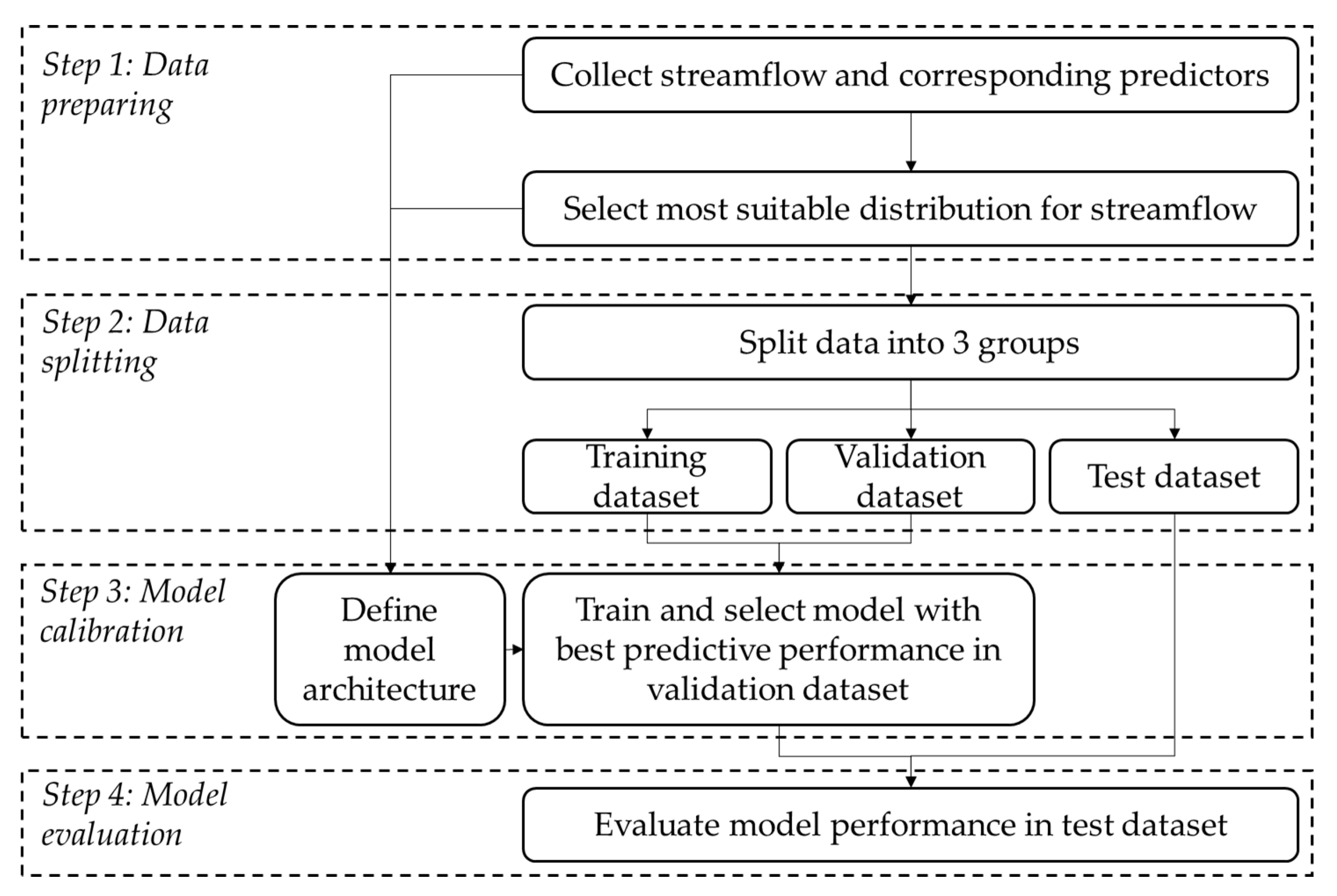
Figure 2.
Study area.
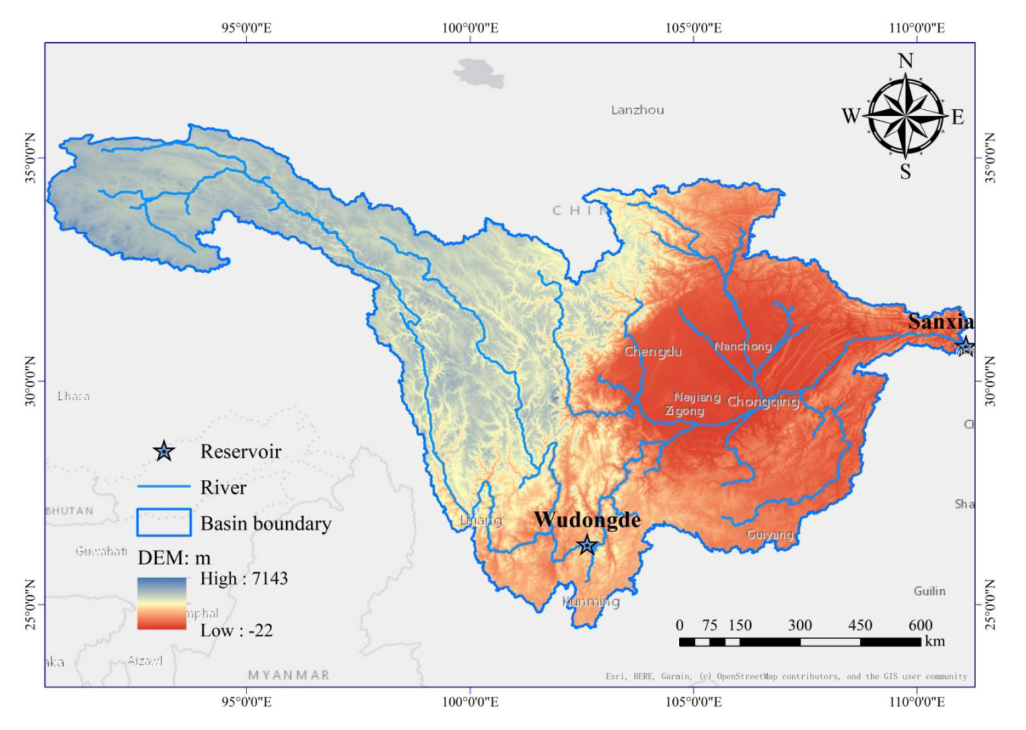
Figure 3.
Distribution fitting figure: (a) Upper WDDR; (b) Upper SXR.
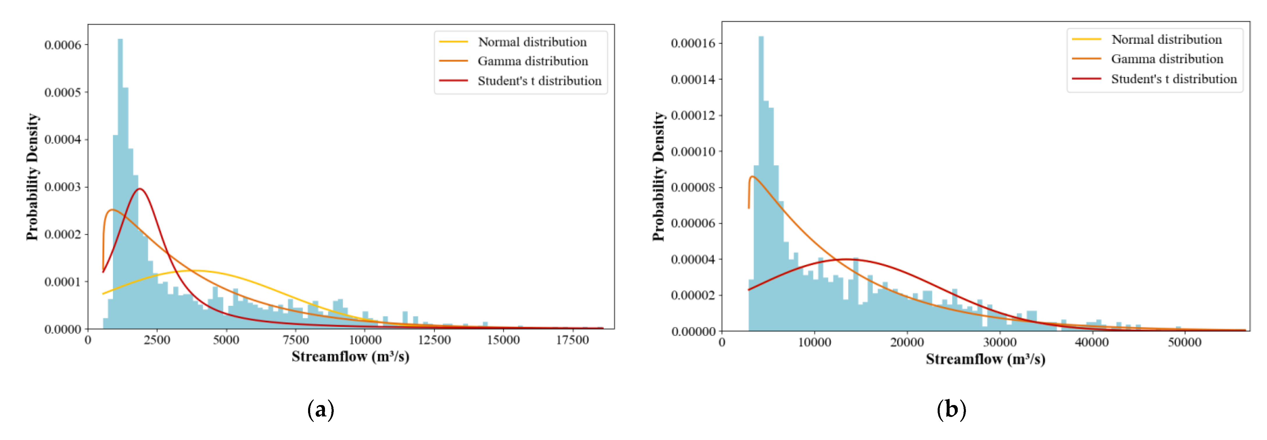
Figure 4.
RMSE of six models across various forecast horizons: (a) Upper WDDR; (b) Upper SXR.
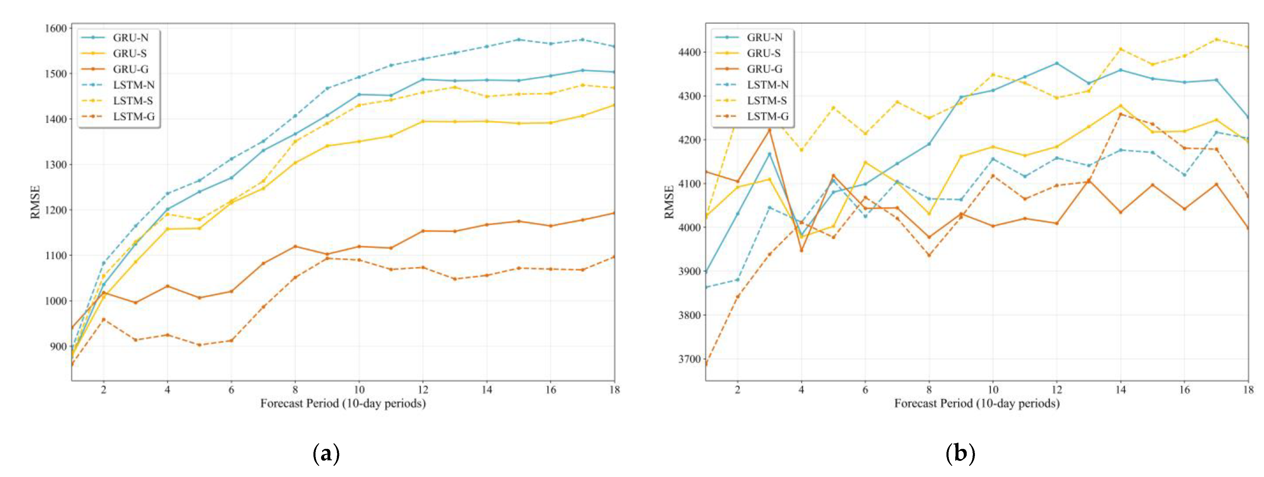
Figure 5.
CRPS of six models across various forecast horizons: (a) Upper WDDR; (b) Upper SXR.

Figure 6.
Predicted streamflow by different models at the 1st forecast period: (a) Upper WDDR; (b) Upper SXR.
Figure 6.
Predicted streamflow by different models at the 1st forecast period: (a) Upper WDDR; (b) Upper SXR.
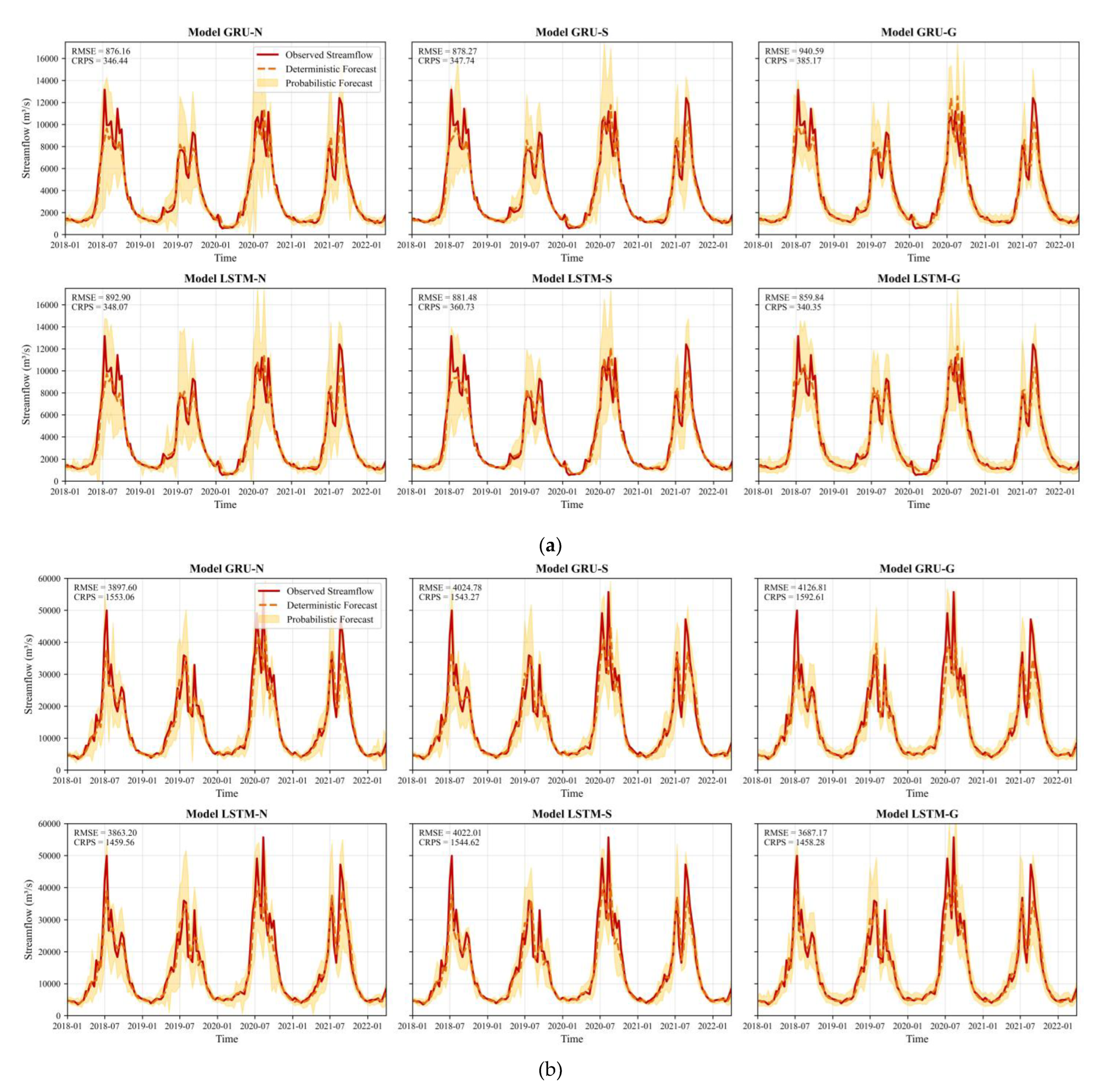
Figure 7.
Predicted streamflow at different forecast periods: (a) Upper WDDR; (b) Upper SXR.
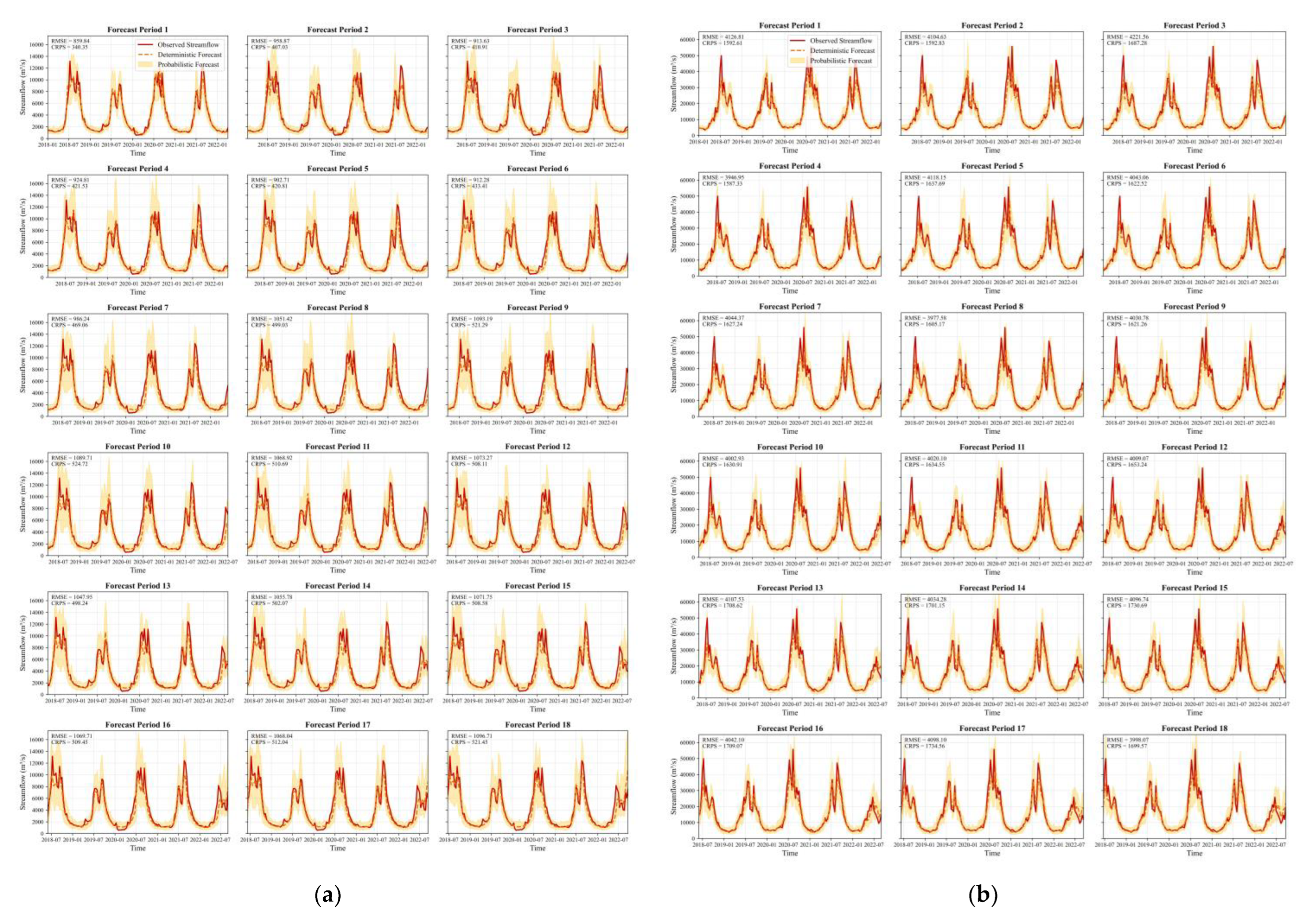

Table 1.
Available data.
| Study area | Variable | Temporal coverage | Temporal scale | Average | Standard deviation |
|---|---|---|---|---|---|
| Upper WDDR | Naturalized streamflow | January 1980 to September 2022 | Ten-day | 3819.97m3/s | 3247.06m3/s |
| Areal mean precipitation | 17.59mm | 18.98mm | |||
| Upper SXR | Naturalized streamflow | January 1980 to September 2022 | Ten-day | 13432.22m3/s | 10016.31m3/s |
| Areal mean precipitation | 22.69mm | 20.36mm |
Table 2.
AIC and BIC values of three distributions for two study areas.
| Study area | Distribution | AIC | BIC |
|---|---|---|---|
| Upper WDDR | Normal | 28574.36 | 28584.99 |
| Student’s t | 28455.62 | 28471.57 | |
| Gamma | 27321.09 | 27337.03 | |
| Upper SXR | Normal | 31960.51 | 31971.14 |
| Student’s t | 31962.46 | 31978.40 | |
| Gamma | 30848.71 | 30864.66 |
Table 3.
Average RMSE on the validation dataset of different models.
| Input configuration | Average RMSE on validation dataset of different models for Upper WDDR area (m3/s) | Average RMSE on validation dataset of different models for Upper SXR area (m3/s) | |
|---|---|---|---|
| Lags of precipitation | 0 | 1277.07 | 3634.55 |
| 0,1 | 1237.00 | 3616.81 | |
| 0,1,2 | 1199.21 | 3481.18 | |
| Lags of streamflow | 1 | 1245.33 | 3577.72 |
| 1,2 | 1230.19 | 3577.31 | |
Table 4.
Predictive performance on the testing dataset of six models with different RNN structures and different probability distribution outputs.
Table 4.
Predictive performance on the testing dataset of six models with different RNN structures and different probability distribution outputs.
| Study area | Evaluation metrics | Model | |||||
|---|---|---|---|---|---|---|---|
| GRU-N | GRU-S | GRU-G | LSTM-N | LSTM-S | LSTM-G | ||
| Upper WDDR | RMSE (m3/s) | 1356.74 | 1282.09 | 1098.98 | 1407.77 | 1331.08 | 1016.54 |
| CRPS (m3/s) | 608.89 | 578.95 | 517.54 | 637.95 | 620.08 | 473.26 | |
| Upper SXR | RMSE (m3/s) | 4217.12 | 4143.33 | 4057.33 | 4091.22 | 4296.16 | 4047.15 |
| CRPS (m3/s) | 1776.92 | 1716.52 | 1654.24 | 1771.43 | 1870.94 | 1717.93 | |
Table 5.
RMSE of six models across various forecast horizons.
| Forecast horizon (10-day periods) | Upper WDDR area | Upper SXR area | ||||||||||
|---|---|---|---|---|---|---|---|---|---|---|---|---|
| GRU-N | GRU-S | GRU-G | LSTM-N | LSTM-S | LSTM-G | GRU-N | GRU-S | GRU-G | LSTM-N | LSTM-S | LSTM-G | |
| 1 | 876.2 | 878.3 | 940.6 | 892.9 | 881.5 | 859.8 | 3897.6 | 4024.8 | 4126.8 | 3863.2 | 4022.0 | 3687.2 |
| 2 | 1035.7 | 1007.6 | 1017.9 | 1083.1 | 1054.9 | 958.9 | 4031.0 | 4091.6 | 4104.6 | 3880.4 | 4254.2 | 3841.5 |
| 3 | 1124.9 | 1085.5 | 995.7 | 1164.5 | 1129.9 | 913.6 | 4167.4 | 4109.5 | 4221.6 | 4045.0 | 4260.8 | 3938.4 |
| 4 | 1201.3 | 1157.9 | 1032.1 | 1235.9 | 1190.4 | 924.8 | 3982.7 | 3978.0 | 3947.0 | 4011.7 | 4176.2 | 4011.2 |
| 5 | 1239.9 | 1159.2 | 1006.4 | 1264.5 | 1178.6 | 902.7 | 4080.1 | 4002.4 | 4118.1 | 4106.4 | 4272.7 | 3977.0 |
| 6 | 1270.4 | 1215.3 | 1020.5 | 1312.1 | 1219.7 | 912.3 | 4098.8 | 4148.2 | 4043.1 | 4024.7 | 4213.8 | 4068.3 |
| 7 | 1330.8 | 1247.1 | 1082.2 | 1351.1 | 1263.2 | 986.2 | 4145.4 | 4102.0 | 4044.4 | 4104.7 | 4285.8 | 4020.6 |
| 8 | 1367.0 | 1303.7 | 1119.5 | 1406.9 | 1350.6 | 1051.4 | 4190.1 | 4031.1 | 3977.6 | 4065.0 | 4249.4 | 3936.1 |
| 9 | 1408.0 | 1340.6 | 1102.5 | 1467.4 | 1390.4 | 1093.2 | 4297.1 | 4161.7 | 4030.8 | 4063.2 | 4283.7 | 4023.0 |
| 10 | 1453.8 | 1350.4 | 1119.3 | 1492.2 | 1430.3 | 1089.7 | 4312.4 | 4183.7 | 4002.9 | 4155.7 | 4348.2 | 4117.6 |
| 11 | 1451.8 | 1362.3 | 1116.0 | 1518.1 | 1441.8 | 1068.9 | 4343.3 | 4163.7 | 4020.1 | 4116.1 | 4329.2 | 4064.6 |
| 12 | 1487.0 | 1394.6 | 1153.5 | 1532.0 | 1458.4 | 1073.3 | 4374.3 | 4184.0 | 4009.1 | 4158.2 | 4295.4 | 4095.5 |
| 13 | 1483.9 | 1394.1 | 1152.8 | 1545.5 | 1469.7 | 1048.0 | 4328.6 | 4229.5 | 4107.5 | 4140.8 | 4311.1 | 4103.9 |
| 14 | 1485.5 | 1394.9 | 1167.4 | 1559.4 | 1449.5 | 1055.8 | 4358.9 | 4277.4 | 4034.3 | 4176.3 | 4406.5 | 4258.0 |
| 15 | 1484.5 | 1390.3 | 1174.9 | 1574.5 | 1454.6 | 1071.8 | 4339.0 | 4217.5 | 4096.7 | 4170.8 | 4371.7 | 4235.7 |
| 16 | 1494.8 | 1391.5 | 1164.6 | 1565.6 | 1456.0 | 1069.7 | 4331.0 | 4219.1 | 4042.1 | 4119.7 | 4391.1 | 4180.6 |
| 17 | 1507.1 | 1407.0 | 1177.8 | 1574.5 | 1474.5 | 1068.0 | 4336.2 | 4245.0 | 4098.1 | 4216.8 | 4428.7 | 4178.2 |
| 18 | 1503.5 | 1430.7 | 1192.9 | 1559.5 | 1468.4 | 1096.7 | 4251.0 | 4194.8 | 3998.1 | 4203.0 | 4411.2 | 4070.5 |
Table 6.
CRPS of six models across various forecast horizons.
| Forecast horizon (10-day periods) | Upper WDDR area | Upper SXR area | ||||||||||
|---|---|---|---|---|---|---|---|---|---|---|---|---|
| GRU-N | GRU-S | GRU-G | LSTM-N | LSTM-S | LSTM-G | GRU-N | GRU-S | GRU-G | LSTM-N | LSTM-S | LSTM-G | |
| 1 | 346.4 | 347.7 | 385.2 | 348.1 | 360.7 | 340.4 | 1553.1 | 1543.3 | 1592.6 | 1459.6 | 1544.6 | 1458.3 |
| 2 | 434.9 | 430.4 | 448.0 | 454.0 | 457.3 | 407.0 | 1660.5 | 1604.5 | 1592.8 | 1558.3 | 1726.7 | 1557.0 |
| 3 | 484.8 | 480.0 | 456.7 | 505.0 | 507.9 | 410.9 | 1730.7 | 1640.8 | 1687.3 | 1659.3 | 1754.6 | 1615.9 |
| 4 | 524.8 | 509.7 | 476.0 | 537.9 | 542.5 | 421.5 | 1665.1 | 1597.8 | 1587.3 | 1683.5 | 1762.0 | 1630.8 |
| 5 | 546.3 | 516.5 | 479.7 | 567.1 | 546.6 | 420.8 | 1698.8 | 1619.6 | 1637.7 | 1744.7 | 1812.4 | 1646.5 |
| 6 | 574.3 | 543.7 | 489.3 | 589.5 | 572.0 | 433.4 | 1697.0 | 1701.7 | 1622.5 | 1724.7 | 1821.5 | 1705.1 |
| 7 | 597.5 | 559.8 | 514.6 | 613.2 | 599.8 | 469.1 | 1730.8 | 1696.1 | 1627.2 | 1772.7 | 1868.5 | 1692.7 |
| 8 | 619.7 | 595.2 | 540.6 | 650.4 | 645.7 | 499.0 | 1762.0 | 1661.0 | 1605.2 | 1743.0 | 1862.3 | 1680.1 |
| 9 | 643.9 | 616.3 | 530.5 | 672.4 | 666.0 | 521.3 | 1822.9 | 1745.4 | 1621.3 | 1774.7 | 1908.1 | 1730.4 |
| 10 | 670.8 | 625.8 | 534.6 | 688.3 | 683.1 | 524.7 | 1834.3 | 1770.1 | 1630.9 | 1825.0 | 1940.2 | 1805.9 |
| 11 | 673.9 | 630.6 | 535.3 | 704.1 | 690.0 | 510.7 | 1840.2 | 1761.5 | 1634.5 | 1831.9 | 1920.9 | 1762.7 |
| 12 | 685.9 | 640.2 | 550.9 | 715.0 | 696.3 | 508.1 | 1855.1 | 1785.1 | 1653.2 | 1865.8 | 1930.1 | 1792.6 |
| 13 | 686.4 | 637.9 | 549.2 | 721.2 | 696.6 | 498.2 | 1848.9 | 1819.6 | 1708.6 | 1860.7 | 1937.2 | 1784.2 |
| 14 | 686.0 | 643.3 | 560.9 | 733.7 | 689.4 | 502.1 | 1850.6 | 1823.0 | 1701.1 | 1896.4 | 1964.7 | 1861.3 |
| 15 | 684.8 | 645.0 | 560.8 | 740.2 | 696.5 | 508.6 | 1871.2 | 1792.8 | 1730.7 | 1860.8 | 1982.0 | 1849.3 |
| 16 | 693.1 | 658.1 | 564.8 | 743.9 | 694.2 | 509.5 | 1841.8 | 1773.2 | 1709.1 | 1853.0 | 1956.9 | 1807.5 |
| 17 | 701.6 | 670.3 | 566.4 | 751.6 | 711.4 | 512.0 | 1878.3 | 1793.6 | 1734.6 | 1894.1 | 1998.1 | 1795.9 |
| 18 | 705.2 | 670.6 | 572.2 | 747.6 | 705.4 | 521.4 | 1843.3 | 1768.5 | 1699.6 | 1877.5 | 1986.0 | 1746.6 |
Disclaimer/Publisher’s Note: The statements, opinions and data contained in all publications are solely those of the individual author(s) and contributor(s) and not of MDPI and/or the editor(s). MDPI and/or the editor(s) disclaim responsibility for any injury to people or property resulting from any ideas, methods, instructions or products referred to in the content. |
© 2025 by the authors. Licensee MDPI, Basel, Switzerland. This article is an open access article distributed under the terms and conditions of the Creative Commons Attribution (CC BY) license (http://creativecommons.org/licenses/by/4.0/).
Copyright: This open access article is published under a Creative Commons CC BY 4.0 license, which permit the free download, distribution, and reuse, provided that the author and preprint are cited in any reuse.


