Analytical Solution of System of FitzHugh-Nagumo Model: A Case Study

System of FitzHugh-Nagumo Model (Xia et al. 2025):

The FitzHugh-Nagumo (FHN) model is proposed by Richard FitzHugh in 1961 which is further refined by Jin-ichi Nagumo. It is a mathematical model that describes the interaction between a membrane potential and a recovery variable.

$${\displaystyle \frac{du}{dt}}=u-{\displaystyle \frac{u^3}{3}}-v+I$$

(1a)

$${\displaystyle \frac{dv}{dt}}=ϵ\left(u+a-bv\right)$$

(1b)

where

$u:$The membrane potential

$v:$ The recovery variable

$I$: External stimulus current applied to the neuron.

$ϵ$: A small constant that separates the timescale where$0<ϵ\ll 1$.

$a,b:$ System parameters governing the dynamical behavior.

Let the initial conditions be

$$u\left(0\right)=c_1,v\left(0\right)=c_2.$$

Let us introduce Adomian Decomposition Method (ADM) to solve the system (1a, b). Let’s define the linear operator and inverse linear operator such that

$$L={\displaystyle \frac{d}{dt}},L^{-1}\left(\cdots \right)={\int }_0^t\left(\cdots \right)d\tau$$

Now, applying linear operator in Eqs. (1a, b), we have

$$Lu=u-{\displaystyle \frac{u^3}{3}}-v+I$$

(2a)

$$Lv=ϵu+ϵa-bϵv$$

(2b)

Then applying inverse linear operator of both sides of (2a, b), we get

$$u\left(t\right)-u\left(0\right)=L^{-1}\left(u\right)-{{\displaystyle \frac{1}{3}}L}^{-1}\left(u^3\right)-L^{-1}\left(v\right)+I{L}^{-1}\left(1\right)$$

$$v\left(t\right)-v\left(0\right)=ϵL^{-1}\left(u\right)+ϵa{L}^{-1}\left(1\right)-bϵL^{-1}\left(v\right)$$

This implies

$$u\left(t\right)=c_1+It+L^{-1}\left(u\right)-L^{-1}\left(v\right)-{{\displaystyle \frac{1}{3}}L}^{-1}\left(u^3\right)$$

(3a)

$$v\left(t\right)=c_2+ϵat+ϵL^{-1}\left(u\right)-bϵL^{-1}\left(v\right)$$

(3b)

Let the solution of $u\left(t\right)$ and $v\left(t\right)$ are

$$u\left(t\right)=\sum _{n=0}^{\infty }{u}_n,v\left(t\right)=\sum _{n=0}^{\infty }{v}_n$$

(4a)

Also, assume that

$$u^3=\sum _{n=0}^{\infty }{A}_n=\sum _{n=0}^{\infty }{\left({\displaystyle \frac{1}{n!}}{\displaystyle \frac{d^n}{d{\lambda }^n}}\left[f\left(\sum _{i=0}^{\infty }{\lambda }^i{u}_i\right)\right]\right)}_{\lambda =0}wheref\left(u\right)=u^3$$

(4b)

Substitute all these values in Eqs. (3a, b), we get

$$\sum _{n=0}^{\infty }{u}_n=c_1+It+L^{-1}\left(\sum _{n=0}^{\infty }{u}_n\right)-L^{-1}\left(\sum _{n=0}^{\infty }{v}_n\right)-{{\displaystyle \frac{1}{3}}L}^{-1}\left(\sum _{n=0}^{\infty }{A}_n\right)$$

(5a)

$$\sum _{n=0}^{\infty }{v}_n=c_2+ϵat+ϵL^{-1}\left(\sum _{n=0}^{\infty }{u}_n\right)-bϵL^{-1}\left(\sum _{n=0}^{\infty }{v}_n\right)$$

(5b)

Let us match terms from both sides, we get

Zeroth Term (n = 0):

$$u_0=c_1+It$$

(6a)

$$v_0=c_2+ϵat$$

(6b)

For $n\ge 0:$

$$u_{n+1}=L^{-1}\left(u_n\right)-L^{-1}\left(v_n\right)-{{\displaystyle \frac{1}{3}}L}^{-1}\left(A_n\right)$$

(7a)

$$v_{n+1}=ϵL^{-1}\left(u_n\right)-bϵL^{-1}\left(v_n\right)$$

(7b)

Also, from Eq. (4b), we have (Dehghan et al. 2010):

$$A_n=\sum _{n=0}^{\infty }{\left({\displaystyle \frac{1}{n!}}{\displaystyle \frac{d^n}{d{\lambda }^n}}\left[f\left(\sum _{i=0}^{\infty }{\lambda }^i{u}_i\right)\right]\right)}_{\lambda =0}wheref\left(u\right)=u^3,n=1,2,3,\cdots$$

It gives

$$\begin{gathered} A_0=u_0^3 \\ {A}_1=3u_0^2{u}_1 \\ {A}_2=3u_0^2{u}_2+3u_0{u}_1^2 \\ {A}_3=3u_0^2{u}_3+6u_0{u}_1{u}_2+u_1^3 \\ {A}_4=3u_0^2{u}_4+6u_0{u}_1{u}_3+3u_0{u}_2^2+3u_1^2{u}_2 \\ \mathrm{and\; so\; on.} \end{gathered}$$

(8)

Now, we will calculate the components: $u_i,v_i,i=1,2,\dots$

Set n = 0 in (7a, b), we get

$$u_1=L^{-1}\left(u_0\right)-L^{-1}\left(v_0\right)-{{\displaystyle \frac{1}{3}}L}^{-1}\left(A_0\right)$$

(9a)

$$v_1=ϵL^{-1}\left(u_0\right)-bϵL^{-1}\left(v_0\right)$$

(9b)

Applying the definition of inverse operator, we get

$$u_1={\int }_0^t\left[u_0\left(\tau \right)-v_0\left(\tau \right)-{\displaystyle \frac{1}{3}}{A}_0\left(\tau \right)\right]d\tau$$

(9a)

$$v_1={\int }_0^t\left[ϵu_0\left(\tau \right)-bϵv_0\left(\tau \right)\right]d\tau$$

(9b)

Substituting the values of$u_0,v_0,A_0$, we get

$$u_1=\left(c_1-c_2-{\displaystyle \frac{1}{3}}{c}_1^3\right)t+{\displaystyle \frac{1}{2}}\left(I-ϵa{-c}_1^{2}I\right)t^2-c_1{I}^2{t}^3-{\displaystyle \frac{1}{12}}{I}^3{t}^4$$

(10a)

$$v_1=\left(ϵc_1-ϵb{c}_2\right)t+{\displaystyle \frac{1}{2}}\left(ϵI-{ϵ}^{2}ab\right)t^2$$

(10b)

Again, set n = 1 in (7a, b), we get

$$u_2=L^{-1}\left(u_1\right)-L^{-1}\left(v_1\right)-{{\displaystyle \frac{1}{3}}L}^{-1}\left(A_1\right)$$

(11a)

$$v_2=ϵL^{-1}\left(u_1\right)-bϵL^{-1}\left(v_1\right)$$

(11b)

Applying the definition of inverse operator, we get

$$u_2={\int }_0^t\left[u_1\left(\tau \right)-v_1\left(\tau \right)-{\displaystyle \frac{1}{3}}{A}_1\left(\tau \right)\right]d\tau$$

(12a)

$$v_2={\int }_0^t\left[ϵu_1\left(\tau \right)-bϵv_1\left(\tau \right)\right]d\tau$$

(12b)

Now, from Eqs. (10a, b), we get

$$u_1=U_{1}t+U_1{t}^2+U_3{t}^3+U_4{t}^4$$

$$v_1=V_{1}t+V_2{t}^2$$

where

$$\begin{gathered} U_1=\left(c_1-c_2-{\displaystyle \frac{1}{3}}{c}_1^3\right),U_2={\displaystyle \frac{1}{2}}\left(I-ϵa{-c}_1^{2}I\right),U_3=-c_1{I}^2,U_4=-{\displaystyle \frac{1}{12}}{I}^3 \\ {V}_1=\left(ϵc_1-ϵb{c}_2\right),V_2={\displaystyle \frac{1}{2}}\left(ϵI-{ϵ}^{2}ab\right) \end{gathered}$$

Substituting the values of$u_1,v_1,A_1$, we get

$$\begin{array}{l}{u}_2={\displaystyle \frac{1}{2}}\left(U_1-V_1-c_1^2{U}_1\right)t^2+{\displaystyle \frac{1}{3}}\left(U_2-V_2-c_1^2{U}_2-2c_{1}I{U}_1\right)t^3\\ \hspace{1em}\hspace{1em}\hspace{1em}\hspace{1em}\hspace{1em}+{\displaystyle \frac{1}{4}}\left(U_3-c_1^2{U}_3-2c_{1}I{U}_2-I^2{U}_1\right)t^4\\ \hspace{1em}\hspace{1em}\hspace{1em}\hspace{1em}\hspace{1em}+{\displaystyle \frac{1}{5}}\left(U_4-c_1^2{U}_4-2c_{1}I{U}_3-I^2{U}_2\right)t^5-{\displaystyle \frac{1}{6}}\left(2c_{1}I{U}_4+I^2{U}_3\right)t^6\\ \hspace{1em}\hspace{1em}\hspace{1em}\hspace{1em}\hspace{1em}-{\displaystyle \frac{1}{7}}{I}^2{U}_4{t}^7\end{array}$$

(13a)

$$v_2={\displaystyle \frac{1}{2}}\left(ϵU_1-ϵb{V}_1\right)t^2+{\displaystyle \frac{1}{3}}\left(ϵU_2-ϵb{V}_2\right)t^3+{\displaystyle \frac{ϵ}{4}}{U}_3{t}^4+{\displaystyle \frac{ϵ}{5}}{U}_4{t}^5$$

(13b)

Hence the approximate analytical solutions are

$$\begin{array}{l}u\left(t\right)\approx \left(c_1+It\right)+\left(U_{1}t+U_1{t}^2+U_3{t}^3+U_4{t}^4\right)\\ \hspace{1em}\hspace{1em}\hspace{1em}\hspace{1em}\hspace{1em}+({\displaystyle \frac{1}{2}}\left(U_1-V_1-c_1^2{U}_1\right)t^2+{\displaystyle \frac{1}{3}}\left(U_2-V_2-c_1^2{U}_2-2c_{1}I{U}_1\right)t^3\\ \hspace{1em}\hspace{1em}\hspace{1em}\hspace{1em}\hspace{1em}+{\displaystyle \frac{1}{4}}\left(U_3-c_1^2{U}_3-2c_{1}I{U}_2-I^2{U}_1\right)t^4\\ \hspace{1em}\hspace{1em}\hspace{1em}\hspace{1em}\hspace{1em}+{\displaystyle \frac{1}{5}}\left(U_4-c_1^2{U}_4-2c_{1}I{U}_3-I^2{U}_2\right)t^5-{\displaystyle \frac{1}{6}}\left(2c_{1}I{U}_4+I^2{U}_3\right)t^6\\ \hspace{1em}\hspace{1em}\hspace{1em}\hspace{1em}\hspace{1em}-{\displaystyle \frac{1}{7}}{I}^2{U}_4{t}^7)+\cdots \end{array}$$

(14a)

$$\begin{array}{l}v\left(t\right)\approx \left(c_2+ϵat\right)+\left(V_{1}t+V_2{t}^2\right)\\ \hspace{1em}\hspace{1em}\hspace{1em}\hspace{1em}\hspace{1em}+\left({\displaystyle \frac{1}{2}}\left(ϵU_1-ϵb{V}_1\right)t^2+{\displaystyle \frac{1}{3}}\left(ϵU_2-ϵb{V}_2\right)t^3+{\displaystyle \frac{ϵ}{4}}{U}_3{t}^4+{\displaystyle \frac{ϵ}{5}}{U}_4{t}^5\right)\\ \hspace{1em}\hspace{1em}\hspace{1em}\hspace{1em}\hspace{1em}+\cdots \end{array}$$

(14b)

Although the Adomian Decomposition Method (ADM) yields explicit approximate analytical expressions for the FitzHugh-Nagumo system, its utility is fundamentally constrained by the mathematical nature of polynomial approximations. While ADM exhibits high accuracy in the short-term regime—effectively capturing the initial transient dynamics and local curvature similar to a Taylor expansion—it suffers from inevitable divergence over longer time horizons. This limitation arises because the FitzHugh-Nagumo model is a dissipative system characterized by a stable limit cycle (sustained oscillations), a behavior that cannot be faithfully represented by a finite polynomial which tends toward infinity.

Let us consider the system (1a, b),$I=0.5,a=-0.7,b=0.8$. Also, $u\left(0\right)=0,v\left(0\right)=0.$ Also, consider the method “odeint” from the scipy.integrate library. Note, “odeint” is a Python wrapper for the LSODA solver. LSODA stands for Livermore Solver for Ordinary Differential equations with Automatic method switching. Using this, we get the following solutions:

Figure 1. Variation of u, v for $ϵ=0.08.$

Figure 1. Variation of u, v for $ϵ=0.08.$

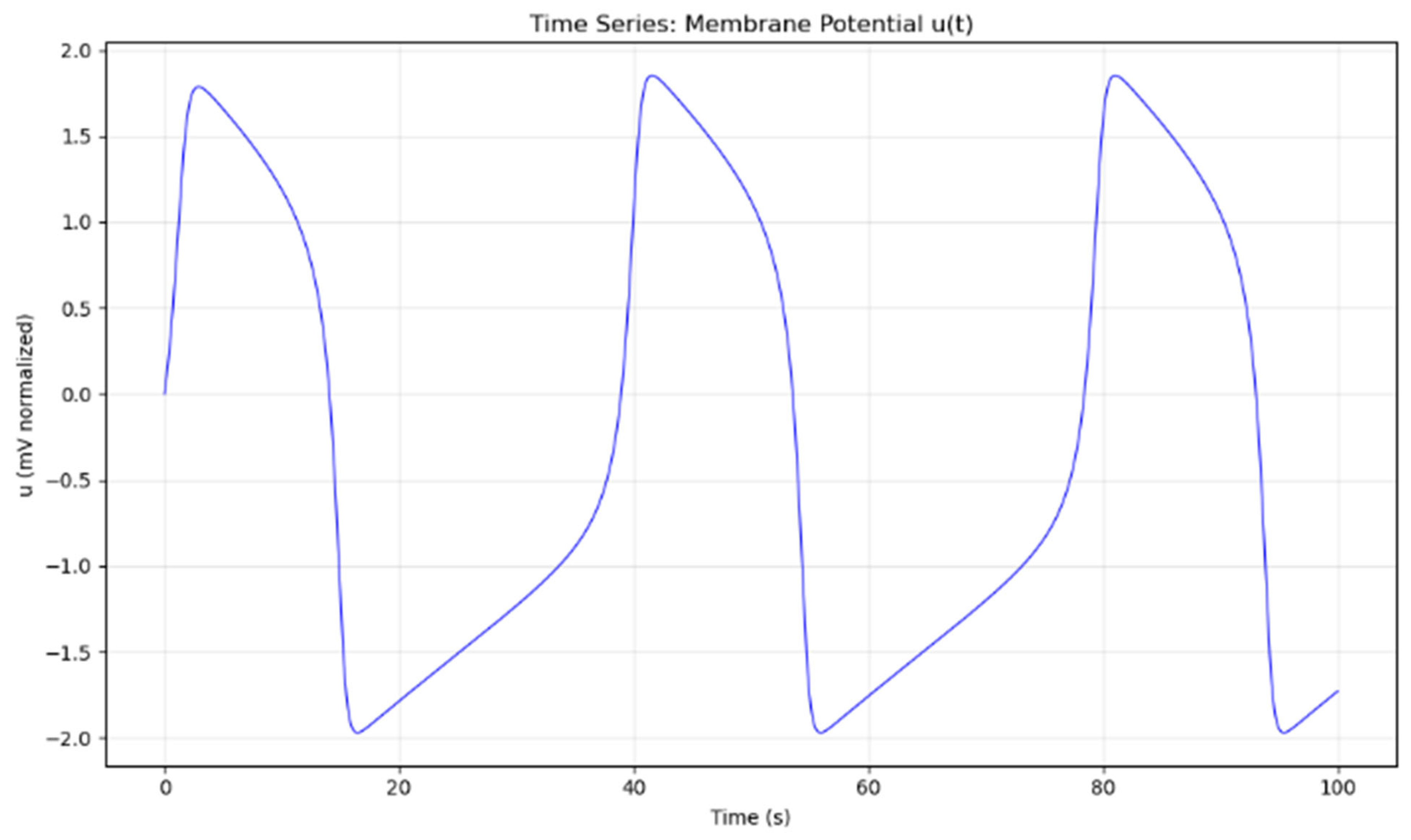
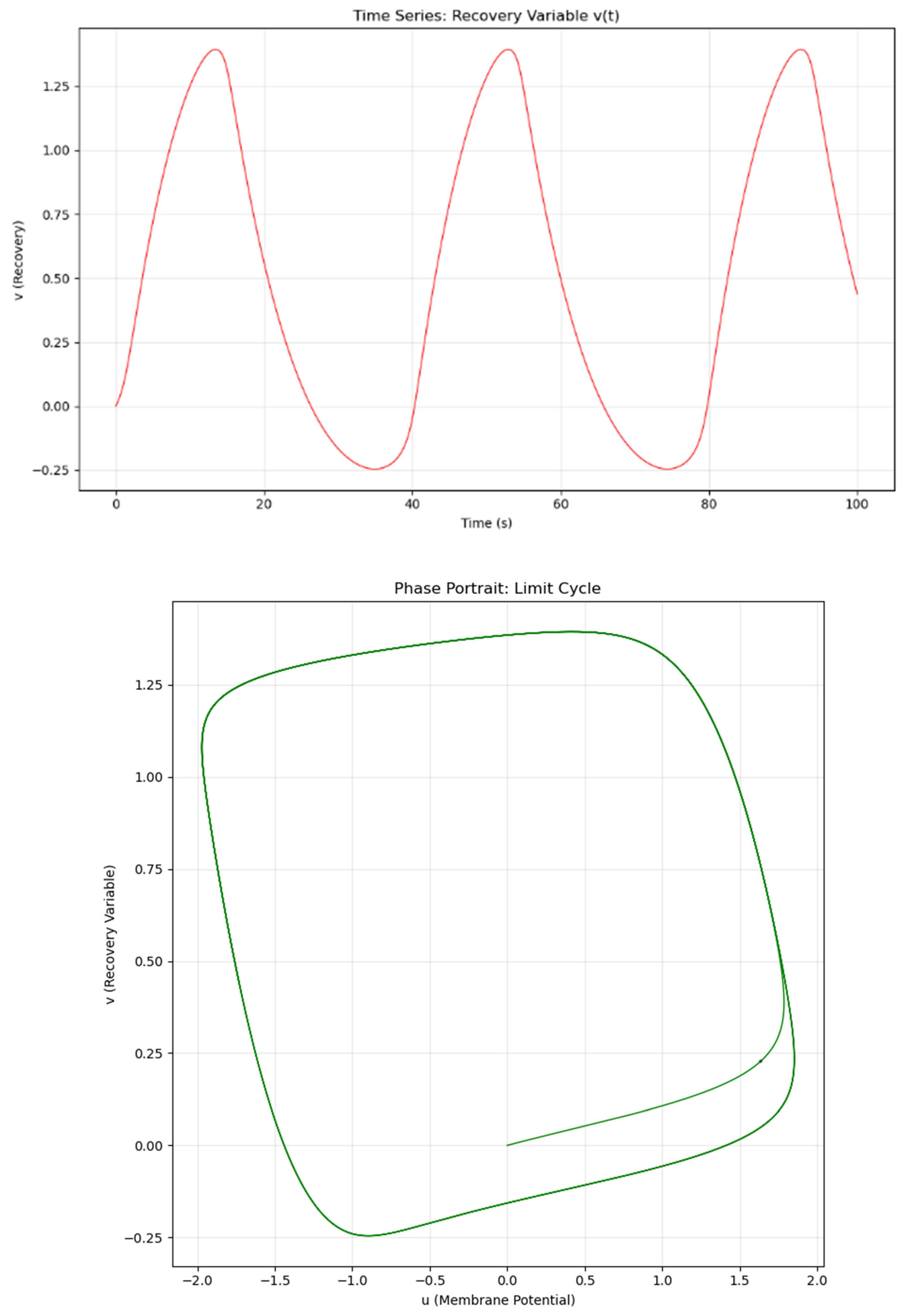
Figure 2. Variation of u, v for $ϵ=0.5.$

Figure 2. Variation of u, v for $ϵ=0.5.$

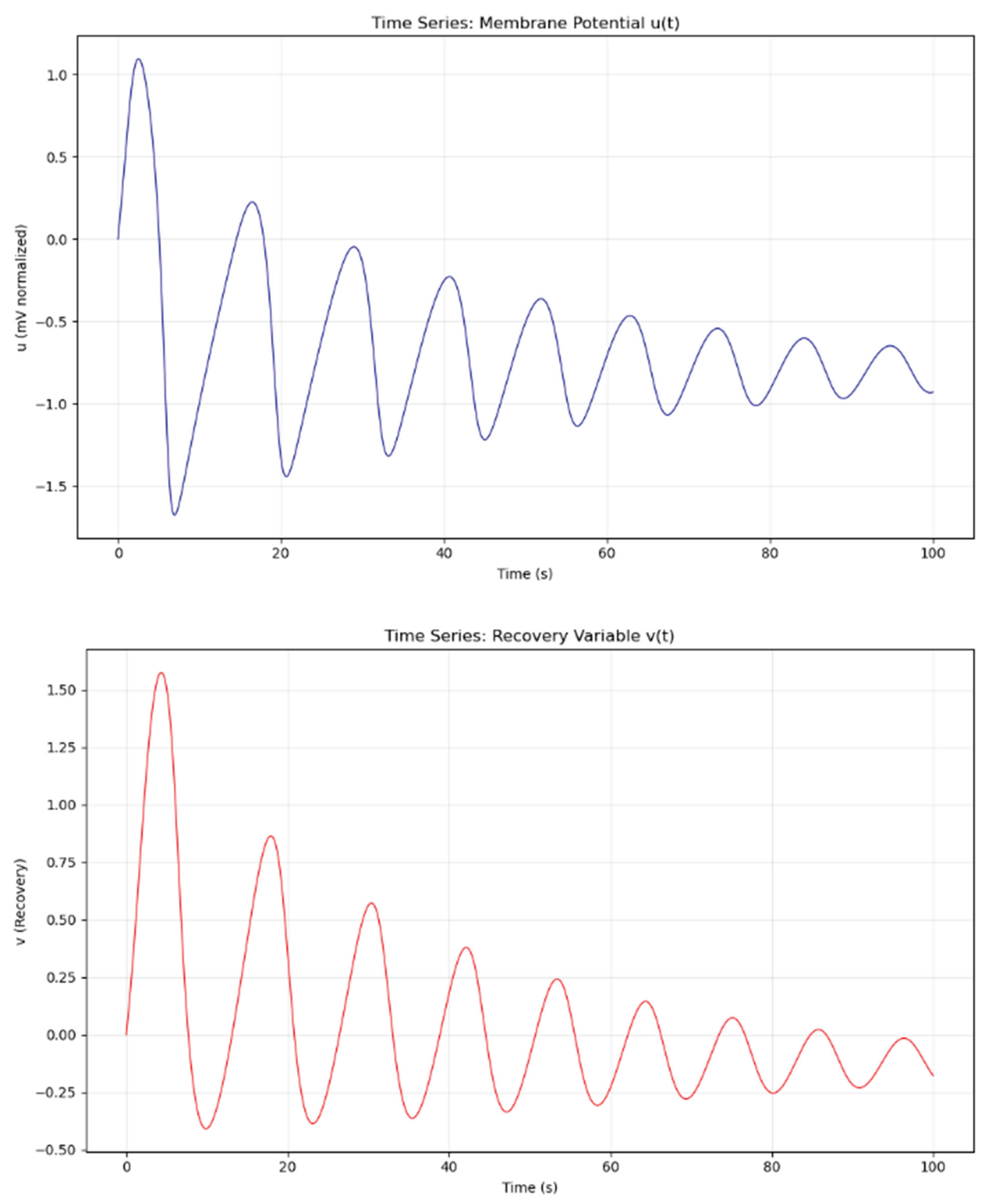
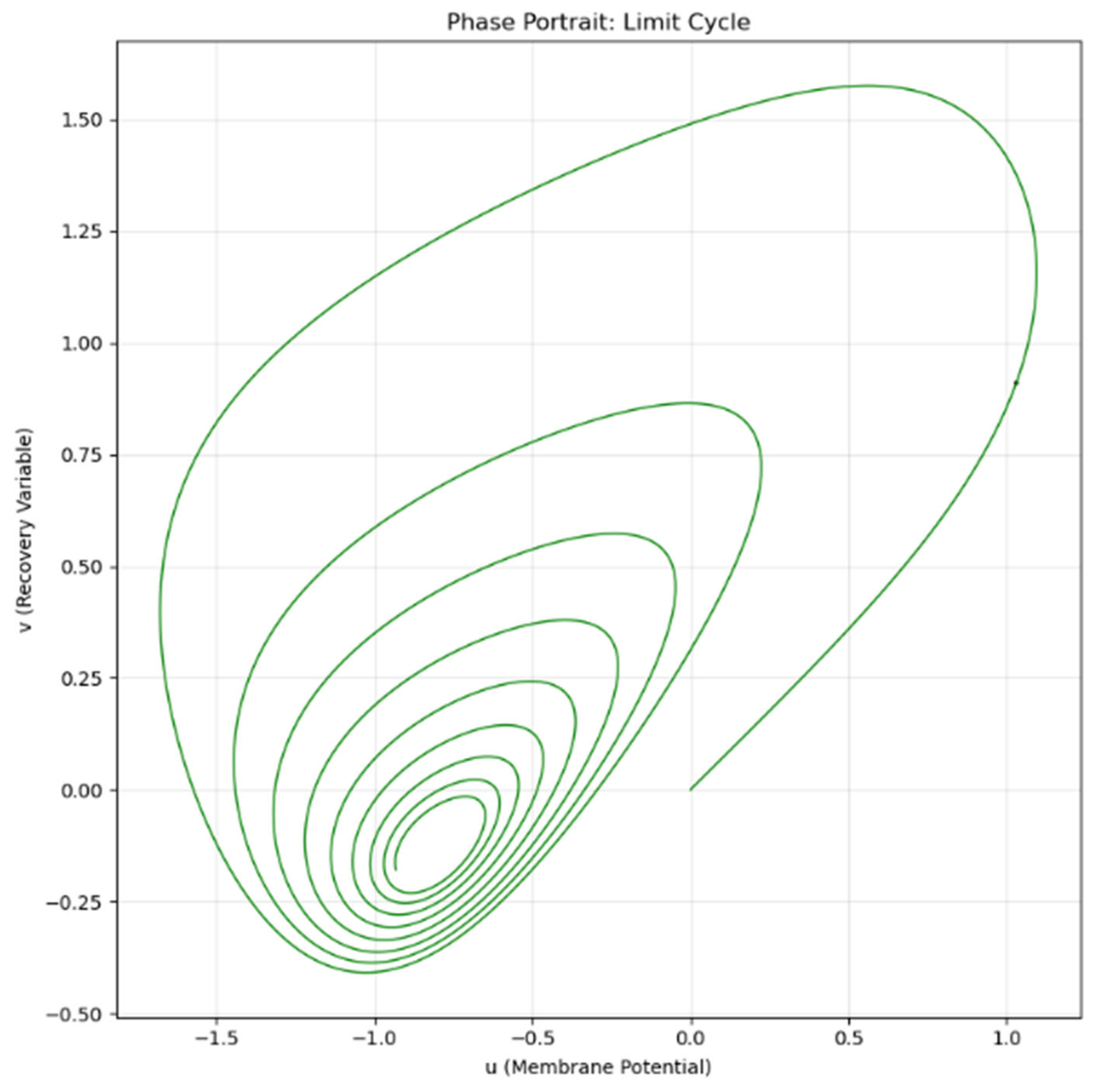
In conclusion, the FitzHugh-Nagumo equations in this study exhibit a stable limit cycle characterized by sustained periodic oscillations. Semi-analytical series methods (such as ADM, HPM, or VIM) rely on polynomial approximations, which inevitably diverge over long time horizons and cannot faithfully reproduce this periodic behavior. Consequently, it is infeasible to obtain a global exact analytical solution for this problem. To accurately capture the long-term dynamics and spiking behavior of the neuron, numerical integration approaches are the necessary and most reliable option.

References

- Dehghan, M.; Heris, J. M.; Saadatmandi, A. Application of semi-analytic methods for the Fitzhugh-Nagumo equation, which models the transmission of nerve impulses. Mathematical Methods in the Applied Sciences 2010, 33(11), 1384–1398. [Google Scholar] [CrossRef]
- Xia, Z.; Huang, X.; Gu, Y.; Saha, S. NeuroPhysNet: A FitzHugh-Nagumo-based physics-informed neural network framework for electroencephalograph (EEG) analysis and motor imagery classification. arXiv. 2025. Available online: https://arxiv.org/abs/2506.13222.
Disclaimer/Publisher’s Note: The statements, opinions and data contained in all publications are solely those of the individual author(s) and contributor(s) and not of MDPI and/or the editor(s). MDPI and/or the editor(s) disclaim responsibility for any injury to people or property resulting from any ideas, methods, instructions or products referred to in the content. |
© 2025 by the authors. Licensee MDPI, Basel, Switzerland. This article is an open access article distributed under the terms and conditions of the Creative Commons Attribution (CC BY) license (http://creativecommons.org/licenses/by/4.0/).
Copyright: This open access article is published under a Creative Commons CC BY 4.0 license, which permit the free download, distribution, and reuse, provided that the author and preprint are cited in any reuse.