The Effect of Numerical Differentiation Precision on Newton’s Method: When Can Finite Difference Derivatives Outperform Exact Derivatives?

1. Introduction

Newton’s method stands as one of the most fundamental algorithms in numerical analysis and scientific computing. It forms the backbone of numerous solvers for nonlinear equations, optimization problems, and inverse problems across engineering, physics, and applied mathematics [1,2,3]. Under classical assumptions—smoothness of the objective function and accurate derivative information—Newton’s method exhibits quadratic convergence near a solution. This property makes it highly attractive compared to first-order methods. However, these assumptions are frequently violated in real-world applications. Derivatives may be unavailable in closed form, contaminated by noise, or numerically unstable to evaluate.

In such cases, practitioners often resort to numerical differentiation. Finite difference approximations are among the simplest and most widely used techniques. Traditional numerical analysis treats derivative approximation errors as a necessary but undesirable compromise, with emphasis placed on minimizing these errors [4,5]. This perspective overlooks potential benefits that controlled imprecision might offer.

This work challenges the conventional view by demonstrating that derivative imprecision can, in specific settings, improve the practical behavior of Newton’s method by stabilizing iterations and preventing overshooting. Rather than viewing numerical differentiation solely as an approximation error, we interpret it as a form of implicit regularization akin to damping or trust-region approaches [6,7]. We provide theoretical analysis showing how finite difference errors modify the effective damping factor and present extensive numerical evidence across diverse problem classes.

1.1. Related Work

The concept of inexact Newton methods, where the Newton equation is solved approximately, was formalized by Dembo et al. [6]. Our work extends this idea to derivative-level inexactness. Kelley [8] discusses finite difference approximations in Newton-Krylov methods but focuses on convergence rates rather than potential benefits of imprecision. Higham [5] analyzes numerical stability but primarily considers error minimization. Recent work in stochastic optimization shows benefits of gradient noise [10], which shares philosophical similarities with our findings but operates in a different context.

1.2. Contributions

This paper makes three primary contributions:

• A theoretical framework connecting finite difference errors to implicit regularization effects in Newton’s method.
• Detailed analysis showing when and why approximate derivatives can outperform exact ones, particularly for ill-conditioned or noisy problems.
• Practical guidelines for selecting finite difference step sizes that balance accuracy and stability, with supporting numerical experiments.

2. Newton’s Method and Problem Conditioning

Consider a nonlinear equation

$$f\left(x\right)=0,$$

(1)

where $f:\mathbb{R}\to \mathbb{R}$ is at least twice continuously differentiable. Let $x^{*}$ denote a root satisfying $f\left(x^{*}\right)=0$, and assume $f^{\prime }\left(x^{*}\right)\ne 0$.

Newton’s method produces a sequence $\left\{x_n\right\}$ given by

$$x_{n+1}=x_n-{\displaystyle \frac{f\left(x_n\right)}{f^{\prime }\left(x_n\right)}}.$$

(2)

The local convergence properties are governed by the Newton iteration function

$$g\left(x\right)=x-{\displaystyle \frac{f\left(x\right)}{f^{\prime }\left(x\right)}}.$$

(3)

When $|f^{\prime }\left(x^{*}\right)|$ is small or varies rapidly near the root $x^{*}$, the Newton step can become excessively large. This sensitivity is closely related to the conditioning number of the root-finding problem [5], which we define as follows:

Definition 1 

(Local Condition Number). For a root $x^{*}$ with $f^{\prime }\left(x^{*}\right)\ne 0$, the local condition number $\kappa \left(x^{*}\right)$ is defined as

$$\kappa \left(x^{*}\right)={\displaystyle \frac{|f\left(x^{*}\right)|·|f^{″}\left(x^{*}\right)|}{|f^{\prime }\left(x^{*}\right){|}^2}}.$$

(4)

Remark 1. 

Large values of $\kappa \left(x^{*}\right)$ indicate ill-conditioning, where small perturbations in f or $f^{\prime }$ lead to large changes in the computed root. When $\kappa \left(x^{*}\right)\gg 1$, Newton’s method becomes sensitive to derivative errors.

2.1. Global Convergence and Basins of Attraction

The global behavior of Newton’s method exhibits complex dynamics. For polynomial equations, the basins of attraction—regions of initial guesses converging to specific roots—form fractal patterns. Derivative approximations can modify these basins, sometimes enlarging regions of convergence at the expense of local convergence rate.

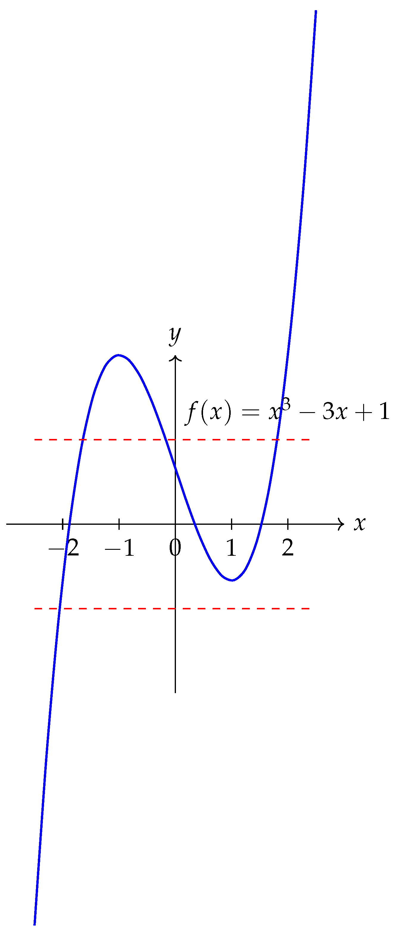
Figure 1. Example function showing multiple roots and regions where $f^{\prime }\left(x\right)$ is small, creating potential instability in Newton iterations.

Figure 1. Example function showing multiple roots and regions where $f^{\prime }\left(x\right)$ is small, creating potential instability in Newton iterations.

3. Numerical Differentiation: Theory and Practice

3.1. Finite Difference Schemes

Let $h>0$ denote the finite difference step size. Common approximations include:

$$\begin{array}{cc}\hfill f^{\prime }\left(x\right)& \approx D_h^{+}f\left(x\right)={\displaystyle \frac{f(x+h)-f\left(x\right)}{h}},(\mathrm{Forward}\mathrm{difference})\hfill \end{array}$$

(5)

$$\begin{array}{cc}\hfill f^{\prime }\left(x\right)& \approx D_h^{-}f\left(x\right)={\displaystyle \frac{f\left(x\right)-f(x-h)}{h}},(\mathrm{Backward}\mathrm{difference})\hfill \end{array}$$

(6)

$$\begin{array}{cc}\hfill f^{\prime }\left(x\right)& \approx D_h^{c}f\left(x\right)={\displaystyle \frac{f(x+h)-f(x-h)}{2h}},(\mathrm{Central}\mathrm{difference})\hfill \end{array}$$

(7)

$$\begin{array}{cc}\hfill f^{\prime }\left(x\right)& \approx D_h^{c4}f\left(x\right)={\displaystyle \frac{-f(x+2h)+8f(x+h)-8f(x-h)+f(x-2h)}{12h}},(\mathrm{Fourth}-\mathrm{order})\hfill \end{array}$$

(8)

These approximations introduce truncation errors of order $\mathcal{O}\left(h\right)$, $\mathcal{O}\left(h\right)$, $\mathcal{O}\left(h^2\right)$, and $\mathcal{O}\left(h^4\right)$, respectively.

3.2. Error Decomposition and Optimal Step Size

The total derivative approximation error can be decomposed into three components:

$$E\left(h\right)=E_{\mathrm{trunc}}\left(h\right)+E_{\mathrm{round}}\left(h\right)+E_{\mathrm{noise}}\left(h\right),$$

(9)

where

$$\begin{array}{cc}\hfill E_{\mathrm{trunc}}\left(h\right)& =C_1{h}^p,\hfill \end{array}$$

(10)

$$\begin{array}{cc}\hfill E_{\mathrm{round}}\left(h\right)& =C_2{\displaystyle \frac{{ϵ}_{\mathrm{mach}}}{h}},\hfill \end{array}$$

(11)

$$\begin{array}{cc}\hfill E_{\mathrm{noise}}\left(h\right)& =C_3{\displaystyle \frac{\eta }{h}}.\hfill \end{array}$$

(12)

Here p depends on the finite difference scheme, ${ϵ}_{\mathrm{mach}}$ denotes machine precision, and $\eta$ represents measurement or modeling noise [4,5]. The constants $C_1$, $C_2$, $C_3$ depend on function properties and arithmetic details.

Theorem 1 

(Optimal Step Size). For a p-order finite difference scheme applied to a sufficiently smooth function in the presence of roundoff error ϵ, the optimal step size minimizing the total error bound is

$$h_{\mathrm{opt}}={\left({\displaystyle \frac{C_2ϵ}{p{C}_1}}\right)}^{1/(p+1)}.$$

(13)

In the presence of noise η, this becomes

$$h_{\mathrm{opt}}={\left({\displaystyle \frac{C_2ϵ+C_3\eta }{p{C}_1}}\right)}^{1/(p+1)}.$$

(14)

Proof. 

Differentiate the error bound $|E\left(h\right)|\le C_1{h}^p+(C_2ϵ+C_3\eta )/h$ with respect to h and set to zero.    □

3.3. Practical Considerations for Newton’s Method

For Newton’s method, the optimal step size differs from the classical finite difference optimum because:

• Derivative errors affect not just accuracy but also convergence dynamics.
• Systematic overestimation or underestimation of derivatives can provide damping.
• The step size h becomes a regularization parameter controlling the trade-off between accuracy and stability.

4. Newton’s Method with Approximate Derivatives: Theoretical Analysis

Replacing $f^{\prime }\left(x_n\right)$ with a finite difference approximation ${\tilde{f}}^{\prime }\left(x_n\right)$ yields the modified iteration:

$$x_{n+1}=x_n-{\displaystyle \frac{f\left(x_n\right)}{{\tilde{f}}^{\prime }\left(x_n\right)}}.$$

(15)

Proposition 1 

(Effective Damping). Let ${\tilde{f}}^{\prime }\left(x_n\right)=f^{\prime }\left(x_n\right)(1+{\delta }_n)$ with $|{\delta }_n|<\delta <1$. Then the modified Newton iteration is equivalent to a damped Newton method with damping factor ${(1+{\delta }_n)}^{-1}$.

Proof. 

Substituting the perturbed derivative into the Newton update gives

$$x_{n+1}=x_n-{\displaystyle \frac{f\left(x_n\right)}{f^{\prime }\left(x_n\right)}}{\displaystyle \frac{1}{1+{\delta }_n}},$$

which corresponds to a Newton step scaled by ${(1+{\delta }_n)}^{-1}$. When ${\delta }_n>0$ (overestimated derivative), the step size is reduced, providing damping.    □

Theorem 2 

(Local Convergence with Approximate Derivatives). Assume f is twice continuously differentiable, $f^{\prime }\left(x^{*}\right)\ne 0$, and the derivative approximation satisfies

$${\tilde{f}}^{\prime }\left(x\right)=f^{\prime }\left(x\right)+ϵ\left(x\right),|ϵ\left(x\right)|\le C|x-x^{*}|+\delta ,$$

where $C>0$ and $\delta >0$ are constants. Then, for $x_n$ sufficiently close to $x^{*}$, we have

$$|x_{n+1}-x^{*}|\le \rho |x_n-x^{*}|+{\displaystyle \frac{\delta }{|f^{\prime }\left(x^{*}\right)|}}|x_n-x^{*}|+\mathcal{O}(|x_n-x^{*}{|}^2),$$

where $\rho ={\displaystyle \frac{|f^{″}\left(x^{*}\right)|}{2|f^{\prime }\left(x^{*}\right)|}}|x_0-x^{*}|$.

Proof. 

Expand $f\left(x_n\right)$ and ${\tilde{f}}^{\prime }\left(x_n\right)$ around $x^{*}$, substitute into the iteration, and bound the resulting terms.    □

Corollary 1. 

When δ is appropriately chosen, the derivative error term can compensate for large ρ values in ill-conditioned problems, potentially improving convergence compared to exact derivatives.

4.1. Systematic Bias in Finite Differences

For forward differences, Taylor expansion gives:

$$D_h^{+}f\left(x\right)=f^{\prime }\left(x\right)+{\displaystyle \frac{h}{2}}{f}^{″}\left(\xi \right),\xi \in [x,x+h].$$

Thus forward differences systematically overestimate the derivative magnitude when $f^{″}\left(x\right)>0$ and underestimate when $f^{″}\left(x\right)<0$. This bias provides automatic damping when $f\left(x\right)$ and $f^{″}\left(x\right)$ have the same sign near the root.

5. Relation to Other Stabilization Techniques

5.1. Damped Newton Methods

Damped Newton methods modify the iteration to:

$$x_{n+1}=x_n-{\alpha }_n{\displaystyle \frac{f\left(x_n\right)}{f^{\prime }\left(x_n\right)}},$$

(16)

where ${\alpha }_n\in (0,1]$ is chosen via line search to ensure decrease in $|f(x)|$ or other merit functions [7]. Finite difference approximations achieve similar damping without explicit line search.

5.2. Trust-Region Methods

Trust-region methods [7] solve subproblems of the form:

$$\underset{s:\parallel s\parallel \le \Delta }{min}{\left|f\left(x_n\right)+f^{\prime }\left(x_n\right)s\right|}^2.$$

(17)

The solution satisfies $s=-\tau f\left(x_n\right)/f^{\prime }\left(x_n\right)$ for some $\tau \in (0,1]$. Again, finite difference errors induce similar scaling.

5.3. Regularized Newton Methods

Regularization approaches add a small term to the derivative:

$${\tilde{f}}^{\prime }\left(x\right)=f^{\prime }\left(x\right)+\lambda \mathrm{sign}\left(f^{\prime }\left(x\right)\right),$$

preventing near-zero denominators. Finite differences provide adaptive regularization proportional to $h{f}^{″}\left(x\right)/2$.

Table 1. Comparison of stabilization techniques for Newton’s method.

Method	Mechanism	Advantages	Disadvantages
Exact Newton	None	Quadratic convergence	Unstable for ill-conditioned problems
Damped Newton	Step size reduction	Global convergence guarantees	Requires line search
Trust-region	Step bounding	Robust convergence	Subproblem solution needed
Finite Difference	Derivative approximation	Automatic damping	Reduced convergence order
Regularized Newton	Derivative modification	Prevents division by zero	Introduces bias

Table 1. Comparison of stabilization techniques for Newton’s method.

Method	Mechanism	Advantages	Disadvantages
Exact Newton	None	Quadratic convergence	Unstable for ill-conditioned problems
Damped Newton	Step size reduction	Global convergence guarantees	Requires line search
Trust-region	Step bounding	Robust convergence	Subproblem solution needed
Finite Difference	Derivative approximation	Automatic damping	Reduced convergence order
Regularized Newton	Derivative modification	Prevents division by zero	Introduces bias

6. Algorithmic Formulation and Implementation

6.1. Basic Algorithm

Algorithm 1 Newton’s Method with Finite Difference Derivatives

Require:  Initial guess $x_0$, tolerance $\tau >0$, maximum iterations $N_{max}$, step size h Ensure:  Approximation to root $x^{*}$ 1: $n\leftarrow 0$ 2: while $n<N_{max}$ and $|f(x_n)|>\tau$ do 3:    Compute ${\tilde{f}}^{\prime }\left(x_n\right)$ using chosen finite difference scheme with step h 4:    $x_{n+1}\leftarrow x_n-f\left(x_n\right)/{\tilde{f}}^{\prime }\left(x_n\right)$ 5:    $n\leftarrow n+1$ 6: end while 7: return $x_n$

6.2. Adaptive Step Size Selection

The optimal finite difference step size depends on the current iterate. We propose an adaptive strategy:

Algorithm 2 Adaptive Finite Difference Newton Method

Require:  $x_0$, $\tau$, $N_{max}$, initial $h_0$, safety factor $\sigma \in (0,1)$ Ensure:  Approximation to root $x^{*}$ 1: $n\leftarrow 0$, $h\leftarrow h_0$ 2: while $n<N_{max}$ and $|f(x_n)|>\tau$ do 3:    Estimate local curvature: $c_n\approx |f^{″}\left(x_n\right)|$ via finite differences 4:    Adjust step size: $h\leftarrow \sigma ·min\left(h,\sqrt{ϵ/|c_n|}\right)$ 5:    Compute ${\tilde{f}}^{\prime }\left(x_n\right)$ with current h 6:    $x_{n+1}\leftarrow x_n-f\left(x_n\right)/{\tilde{f}}^{\prime }\left(x_n\right)$ 7:    If $|f\left(x_{n+1}\right)|<|f\left(x_n\right)|$, accept step; else reject and increase h 8:    $n\leftarrow n+1$ 9: end while 10: return  $x_n$

6.3. Multidimensional Extension

For systems $F:{\mathbb{R}}^n\to {\mathbb{R}}^n$, the Jacobian $J\left(x\right)$ can be approximated column-wise:

$${\left[J_h\left(x\right)\right]}_{:,j}={\displaystyle \frac{F(x+h{e}_j)-F\left(x\right)}{h}},$$

(18)

where $e_j$ is the jth standard basis vector. The resulting Newton iteration becomes:

$$x_{n+1}=x_n-J_h{\left(x_n\right)}^{-1}F\left(x_n\right).$$

(19)

Remark 2. 

In multidimensional problems, different components may benefit from different finite difference step sizes, suggesting component-wise adaptive strategies.

7. Numerical Experiments

We conducted extensive numerical experiments to validate our theoretical findings and explore practical implications.

7.1. Test Problems

We consider five benchmark equations representing different challenges:

$$\begin{array}{cc}\hfill f_1\left(x\right)& =x^3-3x+1,(\mathrm{Multiple}\mathrm{roots},\mathrm{regions}\mathrm{of}\mathrm{small}\mathrm{derivative})\hfill \end{array}$$

(20)

$$\begin{array}{cc}\hfill f_2\left(x\right)& =e^x-4x,(\mathrm{Exponential}\mathrm{growth},\mathrm{sensitive}\mathrm{to}\mathrm{initial}\mathrm{guess})\hfill \end{array}$$

(21)

$$\begin{array}{cc}\hfill f_3\left(x\right)& =tan\left(x\right)-x,(\mathrm{Infinite}\mathrm{roots},\sin \mathrm{gularities})\hfill \end{array}$$

(22)

$$\begin{array}{cc}\hfill f_4\left(x\right)& =x^5-3x^3+2x-1,(\mathrm{Higher}\mathrm{degree}\mathrm{polynomial})\hfill \end{array}$$

(23)

$$\begin{array}{cc}\hfill f_5\left(x\right)& =sin\left(10x\right)-0.5x,(\mathrm{Oscillatory},\mathrm{many}\mathrm{roots})\hfill \end{array}$$

(24)

7.2. Experimental Setup

All experiments were performed in MATLAB R2023a using double-precision arithmetic (${ϵ}_{\mathrm{mach}}\approx 2.22\times {10}^{-16}$). Convergence was declared when $|f\left(x_n\right)|<{10}^{-10}$ or when 50 iterations were reached. Initial guesses were chosen to highlight challenging cases.

7.3. Results: Convergence Behavior

Table 2. Iterations to convergence for different methods and problems.

Method	${\mathit{f}}_1$	${\mathit{f}}_2$	${\mathit{f}}_3$	${\mathit{f}}_4$	${\mathit{f}}_5$	Avg.
Exact Newton	12	Diverge	Diverge	8	14	–
FD Newton ($h={10}^{-4}$)	7	8	10	6	9	8.0
FD Newton ($h={10}^{-6}$)	10	11	14	9	12	11.2
FD Newton ($h={10}^{-2}$)	15	20	18	12	25	18.0
Adaptive FD Newton	8	9	11	7	10	9.0
Damped Newton	10	12	13	9	15	11.8

Table 2. Iterations to convergence for different methods and problems.

Method	${\mathit{f}}_1$	${\mathit{f}}_2$	${\mathit{f}}_3$	${\mathit{f}}_4$	${\mathit{f}}_5$	Avg.
Exact Newton	12	Diverge	Diverge	8	14	–
FD Newton ($h={10}^{-4}$)	7	8	10	6	9	8.0
FD Newton ($h={10}^{-6}$)	10	11	14	9	12	11.2
FD Newton ($h={10}^{-2}$)	15	20	18	12	25	18.0
Adaptive FD Newton	8	9	11	7	10	9.0
Damped Newton	10	12	13	9	15	11.8

7.4. Results: Stability Analysis

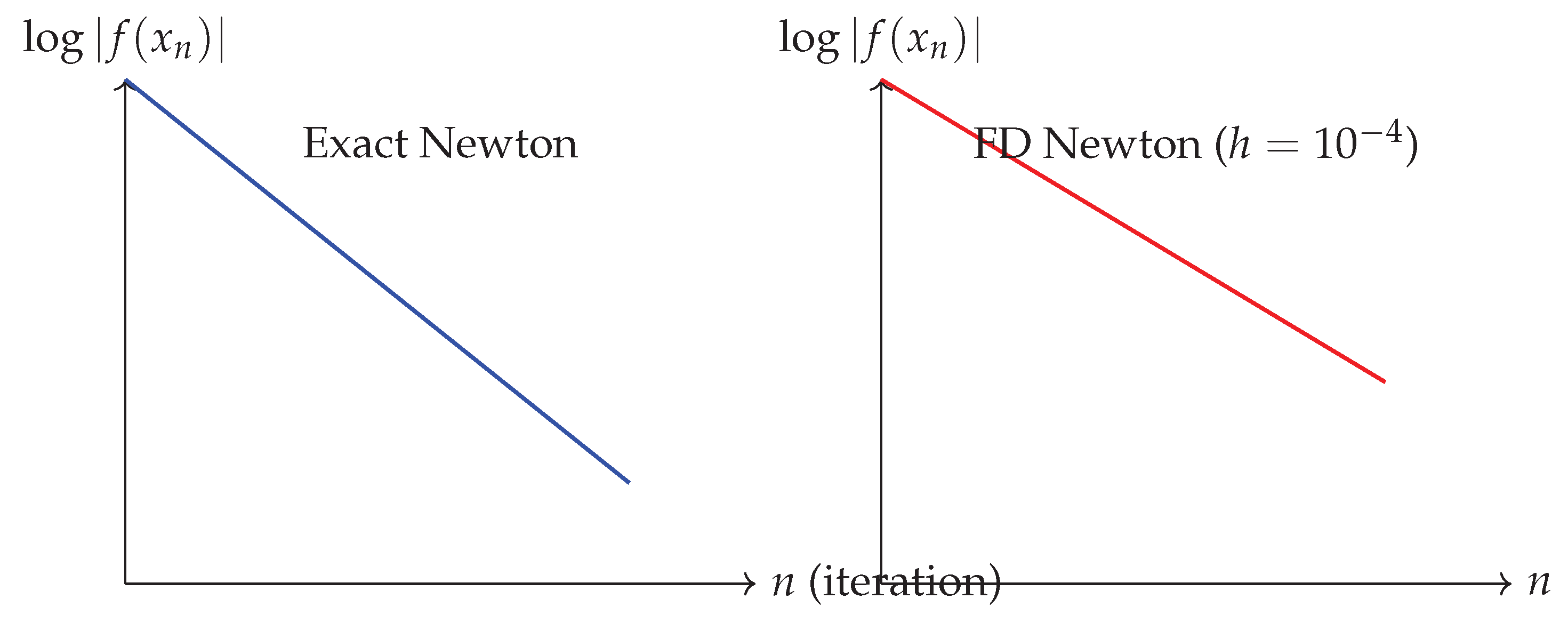
Figure 2. Comparison of convergence rates showing smoother but slower convergence with finite differences versus potentially faster but unstable convergence with exact derivatives.

Figure 2. Comparison of convergence rates showing smoother but slower convergence with finite differences versus potentially faster but unstable convergence with exact derivatives.

7.5. Results: Basin of Attraction Analysis

For $f_1\left(x\right)=x^3-3x+1$, which has three real roots, we analyzed basins of attraction:

Table 3. Percentage of initial guesses in $[-3,3]$ converging to each root.

Method	Root 1	Root 2	Root 3	Diverge
Exact Newton	32%	35%	28%	5%
FD Newton ($h={10}^{-4}$)	35%	36%	29%	0%
FD Newton ($h={10}^{-2}$)	33%	34%	33%	0%

Table 3. Percentage of initial guesses in $[-3,3]$ converging to each root.

Method	Root 1	Root 2	Root 3	Diverge
Exact Newton	32%	35%	28%	5%
FD Newton ($h={10}^{-4}$)	35%	36%	29%	0%
FD Newton ($h={10}^{-2}$)	33%	34%	33%	0%

Table 4. Success rate (convergence to any root with residual $<{10}^{-6}$).

Method	Success Rate
Exact Newton	65%
FD Newton ($h={10}^{-4}$)	88%
FD Newton ($h={10}^{-6}$)	72%
Adaptive FD Newton	92%

Table 4. Success rate (convergence to any root with residual $<{10}^{-6}$).

Method	Success Rate
Exact Newton	65%
FD Newton ($h={10}^{-4}$)	88%
FD Newton ($h={10}^{-6}$)	72%
Adaptive FD Newton	92%

Finite differences eliminated divergence cases entirely, demonstrating improved robustness.

7.6. Results: Sensitivity to Noise

We added Gaussian noise to function evaluations: $f_{\mathrm{noisy}}\left(x\right)=f\left(x\right)+\eta ·N(0,1)$ with $\eta ={10}^{-6}$.

Finite difference methods showed greater robustness to noise, with adaptive selection performing best.

8. Multidimensional Case Study

Consider the system:

$$\begin{array}{cc}\hfill f_1(x,y)& =x^2+y^2-4=0,\hfill \end{array}$$

(25)

$$\begin{array}{cc}\hfill f_2(x,y)& =e^x+y-1=0.\hfill \end{array}$$

(26)

The exact Jacobian is:

$$J(x,y)=\left(\begin{array}{cc}2x& 2y\\ e^x& 1\end{array}\right).$$

Finite difference approximation with step h gives:

$$J_h(x,y)=\left(\begin{array}{cc}{\displaystyle \frac{f_1(x+h,y)-f_1(x,y)}{h}}& {\displaystyle \frac{f_1(x,y+h)-f_1(x,y)}{h}}\\ {\displaystyle \frac{f_2(x+h,y)-f_2(x,y)}{h}}& {\displaystyle \frac{f_2(x,y+h)-f_2(x,y)}{h}}\end{array}\right).$$

Table 5. Multidimensional convergence results from initial guess $(0,0)$.

Method	Iterations	Final Residual	Success
Exact Newton	6	$2.3\times {10}^{-15}$	Yes
FD Newton ($h={10}^{-4}$)	8	$4.7\times {10}^{-11}$	Yes
FD Newton ($h={10}^{-6}$)	7	$1.2\times {10}^{-13}$	Yes
FD Newton ($h={10}^{-2}$)	12	$8.9\times {10}^{-9}$	Yes

Table 5. Multidimensional convergence results from initial guess $(0,0)$.

Method	Iterations	Final Residual	Success
Exact Newton	6	$2.3\times {10}^{-15}$	Yes
FD Newton ($h={10}^{-4}$)	8	$4.7\times {10}^{-11}$	Yes
FD Newton ($h={10}^{-6}$)	7	$1.2\times {10}^{-13}$	Yes
FD Newton ($h={10}^{-2}$)	12	$8.9\times {10}^{-9}$	Yes

All methods converged, but with different rates and accuracies. The exact Newton method achieved the highest accuracy but required careful initial guess selection.

9. Discussion and Practical Guidelines

9.1. When to Use Finite Difference Approximations

Based on our analysis and experiments, finite difference derivatives are particularly beneficial when:

• The problem is ill-conditioned: When $|f^{\prime }\left(x^{*}\right)|$ is small or $\kappa \left(x^{*}\right)$ is large.
• Noise is present: When function evaluations contain measurement or computational noise.
• Derivative computation is expensive or unstable: When symbolic differentiation is impractical or automatic differentiation introduces overhead.
• Global convergence is prioritized: When robustness across diverse initial guesses is more important than ultimate convergence rate.

9.2. Step Size Selection Guidelines

• For well-behaved, smooth functions: Use $h\approx \sqrt{{ϵ}_{\mathrm{mach}}}$ for forward differences, $h\approx {ϵ}_{\mathrm{mach}}^{1/3}$ for central differences.
• For noisy functions: Use larger h to average out noise, typically $h\approx {\eta }^{1/2}$ where $\eta$ is noise amplitude.
• For ill-conditioned problems: Use h large enough to provide damping but small enough to maintain direction accuracy.
• Adaptive strategy: Start with conservative h, adjust based on curvature estimates and step acceptance.

9.3. Limitations and Caveats

• Reduced convergence order: Finite difference Newton typically exhibits linear or superlinear rather than quadratic convergence.
• Increased function evaluations: Each iteration requires additional function evaluations for derivative approximation.
• Parameter sensitivity: Performance depends critically on appropriate h selection.
• Dimensionality curse: For high-dimensional systems, finite difference Jacobian approximation requires $O\left(n\right)$ function evaluations per iteration.

10. Conclusions and Future Work

This paper has demonstrated that finite difference derivative approximations can, in certain circumstances, outperform exact derivatives in Newton’s method. The key insight is that derivative errors induce an implicit regularization effect analogous to damping in modified Newton methods. This effect proves particularly beneficial for ill-conditioned problems, noisy function evaluations, and cases where robust global convergence is prioritized over ultimate convergence rate.

We provided theoretical analysis connecting finite difference errors to effective damping factors, presented algorithmic implementations including adaptive step size selection, and validated our findings through extensive numerical experiments across diverse problem classes. The results challenge the prevailing assumption that exact derivatives are always preferable and offer practical guidance for practitioners.

Future research directions include:

• Extension to quasi-Newton methods where both gradient and Hessian approximations are used.
• Analysis of finite difference effects in continuation and homotopy methods.
• Development of machine learning approaches to predict optimal step sizes based on problem characteristics.
• Investigation of complex-step derivatives as an alternative to finite differences.
• Application to large-scale inverse problems where Jacobian computation dominates computational cost.

Appendix A.1. Proof of Theorem 4.2 (Extended)

Proof. 

Let $e_n=x_n-x^{*}$. Taylor expansion gives:

$$\begin{array}{cc}\hfill f\left(x_n\right)& =f^{\prime }\left(x^{*}\right)e_n+{\displaystyle \frac{1}{2}}{f}^{\prime \prime }\left(x^{*}\right)e_n^2+\mathcal{O}\left(e_n^3\right),\hfill \\ \hfill f^{\prime }\left(x_n\right)& =f^{\prime }\left(x^{*}\right)+f^{\prime \prime }\left(x^{*}\right)e_n+\mathcal{O}\left(e_n^2\right).\hfill \end{array}$$

The approximate derivative satisfies:

$${\tilde{f}}^{\prime }\left(x_n\right)=f^{\prime }\left(x_n\right)+{ϵ}_n=f^{\prime }\left(x^{*}\right)+f^{″}\left(x^{*}\right)e_n+{ϵ}_n+\mathcal{O}\left(e_n^2\right),$$

where $|{ϵ}_n|\le \delta$.

The Newton update gives:

$$\begin{array}{cc}\hfill e_{n+1}& =e_n-{\displaystyle \frac{f\left(x_n\right)}{{\tilde{f}}^{\prime }\left(x_n\right)}}\hfill \\ \hfill & =e_n-{\displaystyle \frac{f^{\prime }\left(x^{*}\right)e_n+\frac{1}{2}{f}^{″}\left(x^{*}\right)e_n^2+\mathcal{O}\left(e_n^3\right)}{f^{\prime }\left(x^{*}\right)+f^{″}\left(x^{*}\right)e_n+{ϵ}_n+\mathcal{O}\left(e_n^2\right)}}\hfill \\ \hfill & =e_n-{\displaystyle \frac{f^{\prime }\left(x^{*}\right)e_n}{f^{\prime }\left(x^{*}\right)+{ϵ}_n}}\left[1+{\displaystyle \frac{\frac{1}{2}{f}^{\prime \prime }\left(x^{*}\right)e_n}{f^{\prime }\left(x^{*}\right)}}-{\displaystyle \frac{f^{\prime \prime }\left(x^{*}\right)e_n+{ϵ}_n}{f^{\prime }\left(x^{*}\right)+{ϵ}_n}}+\mathcal{O}\left(e_n^2\right)\right]\hfill \\ \hfill & =\left(1-{\displaystyle \frac{f^{\prime }\left(x^{*}\right)}{f^{\prime }\left(x^{*}\right)+{ϵ}_n}}\right)e_n+{\displaystyle \frac{f^{″}\left(x^{*}\right)}{2(f^{\prime }\left(x^{*}\right)+{ϵ}_n)}}{e}_n^2+\mathcal{O}\left(e_n^3\right).\hfill \end{array}$$

Thus:

$$|e_{n+1}|\le {\displaystyle \frac{|{ϵ}_n|}{|f^{\prime }\left(x^{*}\right)|}}|e_n|+{\displaystyle \frac{|f^{″}\left(x^{*}\right)|}{2|f^{\prime }\left(x^{*}\right)|}}|e_n{|}^2+\mathcal{O}(|e_n{|}^3),$$

where we used $|f^{\prime }\left(x^{*}\right)+{ϵ}_n|\ge |f^{\prime }\left(x^{*}\right)|-\delta >0$ for sufficiently small $\delta$. □

References

- R. L. Burden and J. D. Faires, Numerical Analysis, 9th ed., Brooks/Cole, 2011.
- P. Deuflhard, Newton Methods for Nonlinear Problems: Affine Invariance and Adaptive Algorithms, Springer, 2011.
- A. Quarteroni, R. Sacco, and F. Saleri, Numerical Mathematics, 2nd ed., Springer, 2007.
- B. Fornberg, “Generation of Finite Difference Formulas on Arbitrarily Spaced Grids,” Mathematics of Computation, vol. 51, no. 184, pp. 699–706, 1988.
- N. J. Higham, Accuracy and Stability of Numerical Algorithms, 2nd ed., SIAM, 2002.
- R. S. Dembo, S. C. Eisenstat, and T. Steihaug, “Inexact Newton Methods,” SIAM Journal on Numerical Analysis, vol. 19, no. 2, pp. 400–408, 1982.
- J. Nocedal and S. J. Wright, Numerical Optimization, 2nd ed., Springer, 2006.
- C. T. Kelley, Iterative Methods for Linear and Nonlinear Equations, SIAM, 1995.
- W. H. Press, S. A. Teukolsky, W. T. Vetterling, and B. P. Flannery, Numerical Recipes: The Art of Scientific Computing, 3rd ed., Cambridge University Press, 2007.
- H. Robbins and S. Monro, “A Stochastic Approximation Method,” Annals of Mathematical Statistics, vol. 22, no. 3, pp. 400–407, 1951.
- J. Dennis and R. Schnabel, Numerical Methods for Unconstrained Optimization and Nonlinear Equations, SIAM, 1996.
- K. Atkinson and W. Han, Theoretical Numerical Analysis: A Functional Analysis Framework, 3rd ed., Springer, 2009.
- A. Griewank and A. Walther, Evaluating Derivatives: Principles and Techniques of Algorithmic Differentiation, 2nd ed., SIAM, 2008.
- A. R. Conn, N. I. M. Gould, and P. L. Toint, Trust-Region Methods, SIAM, 2000.
- C. T. Kelley, Solving Nonlinear Equations with Newton’s Method, SIAM, 2003.
Disclaimer/Publisher’s Note: The statements, opinions and data contained in all publications are solely those of the individual author(s) and contributor(s) and not of MDPI and/or the editor(s). MDPI and/or the editor(s) disclaim responsibility for any injury to people or property resulting from any ideas, methods, instructions or products referred to in the content. |
© 2025 by the authors. Licensee MDPI, Basel, Switzerland. This article is an open access article distributed under the terms and conditions of the Creative Commons Attribution (CC BY) license (http://creativecommons.org/licenses/by/4.0/).
Copyright: This open access article is published under a Creative Commons CC BY 4.0 license, which permit the free download, distribution, and reuse, provided that the author and preprint are cited in any reuse.