First-Order Ordinary Differential Equations: Comprehensive Theory, Methods, and Modern Applications

1. Introduction and Historical Context

1.1. Historical Development

The study of differential equations originated in the 17th century with the work of Isaac Newton and Gottfried Leibniz, who developed calculus as a language for describing continuous change. Early applications focused on physical problems: planetary motion, optics, and mechanics. The 18th century saw systematic development by Euler, Bernoulli, and Lagrange, establishing many fundamental solution methods still in use today.

1.2. Mathematical Formulation

A first-order ordinary differential equation expresses a relationship between an unknown function $y\left(t\right)$, its derivative $dy/dt$, and the independent variable t:

$$F\left(t,y,{\displaystyle \frac{dy}{dt}}\right)=0\mathrm{or}\mathrm{equivalently}{\displaystyle \frac{dy}{dt}}=f(t,y)$$

(1.1)

The general solution typically contains one arbitrary constant, determined by an initial condition:

$$y\left(t_0\right)=y_0$$

(1.2)

Theorem 1 

(Picard–Lindelöf Existence and Uniqueness). Consider the initial value problem (1.1)-(1.2). If $f(t,y)$ is continuous in a rectangle $R=\{(t,y):|t-t_0|\le a,|y-y_0|\le b\}$ and satisfies a Lipschitz condition in y:

$$|f(t,y_1)-f(t,y_2)|\le L|y_1-y_2|\forall (t,y_1),(t,y_2)\in R$$

then there exists a unique solution $y\left(t\right)$ on some interval $|t-t_0|\le h$, where $h=min(a,b/M)$ with $M={max}_{(t,y)\in R}\left|f(t,y)\right|$.

1.3. Classification of First-Order ODEs

First-order ODEs can be categorized based on their structure:

Table 1. Classification of first-order ODEs.

Type	General Form	Characteristics
Separable	${\displaystyle \frac{dy}{dt}}=g\left(t\right)h\left(y\right)$	Variables can be separated
Linear	${\displaystyle \frac{dy}{dt}}+P\left(t\right)y=Q\left(t\right)$	Linear in y and $dy/dt$
Exact	$M(t,y)dt+N(t,y)dy=0$	${\displaystyle \frac{\partial M}{\partial y}}={\displaystyle \frac{\partial N}{\partial t}}$
Bernoulli	${\displaystyle \frac{dy}{dt}}+P\left(t\right)y=Q\left(t\right)y^n$	Nonlinear but reducible to linear
Homogeneous	${\displaystyle \frac{dy}{dt}}=f\left({\displaystyle \frac{y}{t}}\right)$	Invariant under scaling

Table 1. Classification of first-order ODEs.

Type	General Form	Characteristics
Separable	${\displaystyle \frac{dy}{dt}}=g\left(t\right)h\left(y\right)$	Variables can be separated
Linear	${\displaystyle \frac{dy}{dt}}+P\left(t\right)y=Q\left(t\right)$	Linear in y and $dy/dt$
Exact	$M(t,y)dt+N(t,y)dy=0$	${\displaystyle \frac{\partial M}{\partial y}}={\displaystyle \frac{\partial N}{\partial t}}$
Bernoulli	${\displaystyle \frac{dy}{dt}}+P\left(t\right)y=Q\left(t\right)y^n$	Nonlinear but reducible to linear
Homogeneous	${\displaystyle \frac{dy}{dt}}=f\left({\displaystyle \frac{y}{t}}\right)$	Invariant under scaling

1.4. Modern Significance

In contemporary science and engineering, first-order ODEs model:

• Population dynamics in ecology
• Chemical kinetics and reaction rates
• Electrical circuits (RC, RL)
• Pharmacokinetics and drug metabolism
• Economic growth models
• Heat transfer and diffusion processes
• Machine learning (gradient descent dynamics)

2. Analytical Solution Methods: Comprehensive Treatment

2.1. Separation of Variables with Advanced Examples

The separation of variables technique applies when the function $f(t,y)$ factors as $g\left(t\right)h\left(y\right)$:

$${\displaystyle \frac{dy}{dt}}=g\left(t\right)h\left(y\right)\Rightarrow \int {\displaystyle \frac{dy}{h\left(y\right)}}=\int g\left(t\right)dt+C$$

(2.1)

Example 2.1: Solve ${\displaystyle \frac{dy}{dt}}=y(1-y^2)$ with $y\left(0\right)=0.5$.

Solution: Separating variables:

$$\int {\displaystyle \frac{dy}{y(1-y^2)}}=\int dt$$

Using partial fractions:

$${\displaystyle \frac{1}{y(1-y^2)}}={\displaystyle \frac{1}{y}}+{\displaystyle \frac{1}{2(1-y)}}-{\displaystyle \frac{1}{2(1+y)}}$$

Integrating:

$$ln\left|y\right|-{\displaystyle \frac{1}{2}}ln|1-y|-{\displaystyle \frac{1}{2}}ln|1+y|=t+C$$

Simplifying:

$$ln\left|{\displaystyle \frac{y}{\sqrt{1-y^2}}}\right|=t+C\Rightarrow {\displaystyle \frac{y}{\sqrt{1-y^2}}}=A{e}^t$$

With $y\left(0\right)=0.5$, $A={\displaystyle \frac{0.5}{\sqrt{1-0.25}}}={\displaystyle \frac{1}{\sqrt{3}}}$. Final solution:

$$y\left(t\right)={\displaystyle \frac{e^t}{\sqrt{3+e^{2t}}}}$$

2.2. Linear Equations: Theory and Applications

The general linear first-order ODE has the form:

$${\displaystyle \frac{dy}{dt}}+P\left(t\right)y=Q\left(t\right)$$

(2.2)

The integrating factor method provides a systematic solution:

$$\mu \left(t\right)=exp\left(\int P\left(t\right)dt\right)$$

(2.3)

Multiplying (2.2) by $\mu \left(t\right)$ gives:

$${\displaystyle \frac{d}{dt}}\left[\mu \left(t\right)y\right]=\mu \left(t\right)Q\left(t\right)$$

Integrating:

$$y\left(t\right)={\displaystyle \frac{1}{\mu \left(t\right)}}\left[\int \mu \left(t\right)Q\left(t\right)dt+C\right]$$

(2.4)

Example 2.2: RL circuit equation: $L{\displaystyle \frac{dI}{dt}}+RI=V\left(t\right)$, where $V\left(t\right)=V_{0}sin\left(\omega t\right)$.

Solution: Rewrite as ${\displaystyle \frac{dI}{dt}}+{\displaystyle \frac{R}{L}}I={\displaystyle \frac{V_0}{L}}sin\left(\omega t\right)$. Integrating factor:

$$\mu \left(t\right)=exp\left(\int {\displaystyle \frac{R}{L}}dt\right)=e^{Rt/L}$$

Solution:

$$I\left(t\right)=e^{-Rt/L}\left[{\displaystyle \frac{V_0}{L}}\int e^{Rt/L}sin\left(\omega t\right)dt+C\right]$$

Evaluating the integral:

$$\int e^{Rt/L}sin\left(\omega t\right)dt={\displaystyle \frac{e^{Rt/L}\left(\frac{R}{L}sin\left(\omega t\right)-\omega cos\left(\omega t\right)\right)}{{\left(\frac{R}{L}\right)}^2+{\omega }^2}}$$

Thus:

$$I\left(t\right)={\displaystyle \frac{V_0}{R^2+{\omega }^2{L}^2}}\left(Rsin\left(\omega t\right)-\omega Lcos\left(\omega t\right)\right)+C{e}^{-Rt/L}$$

2.3. Exact Equations and Integrating Factors

The differential form $M(t,y)dt+N(t,y)dy=0$ is exact if:

$${\displaystyle \frac{\partial M}{\partial y}}={\displaystyle \frac{\partial N}{\partial t}}$$

(2.5)

If exact, there exists $\Psi (t,y)$ such that:

$$d\Psi =Mdt+Ndy=0\Rightarrow \Psi (t,y)=C$$

Example 2.3: Solve $(2ty+3t^2)dt+(t^2+4y^3)dy=0$.

Solution: Check exactness:

$${\displaystyle \frac{\partial M}{\partial y}}={\displaystyle \frac{\partial }{\partial y}}(2ty+3t^2)=2t$$

$${\displaystyle \frac{\partial N}{\partial t}}={\displaystyle \frac{\partial }{\partial t}}(t^2+4y^3)=2t$$

Equal, so exact. Find $\Psi$:

$${\displaystyle \frac{\partial \Psi }{\partial t}}=2ty+3t^2\Rightarrow \Psi =t^{2}y+t^3+h\left(y\right)$$

$${\displaystyle \frac{\partial \Psi }{\partial y}}=t^2+h^{\prime }\left(y\right)=t^2+4y^3\Rightarrow h^{\prime }\left(y\right)=4y^3\Rightarrow h\left(y\right)=y^4$$

Thus $\Psi (t,y)=t^{2}y+t^3+y^4=C$.

2.4. Bernoulli Equations and Transformations

The Bernoulli equation:

$${\displaystyle \frac{dy}{dt}}+P\left(t\right)y=Q\left(t\right)y^n,n\ne 0,1$$

(2.6)

Substituting $z=y^{1-n}$ gives a linear equation:

$${\displaystyle \frac{dz}{dt}}+(1-n)P\left(t\right)z=(1-n)Q\left(t\right)$$

2.5. Riccati Equations

The Riccati equation:

$${\displaystyle \frac{dy}{dt}}=a\left(t\right)y^2+b\left(t\right)y+c\left(t\right)$$

(2.7)

If a particular solution $y_p\left(t\right)$ is known, the substitution $y=y_p+{\displaystyle \frac{1}{z}}$ transforms it to linear.

3. Qualitative Analysis and Stability Theory

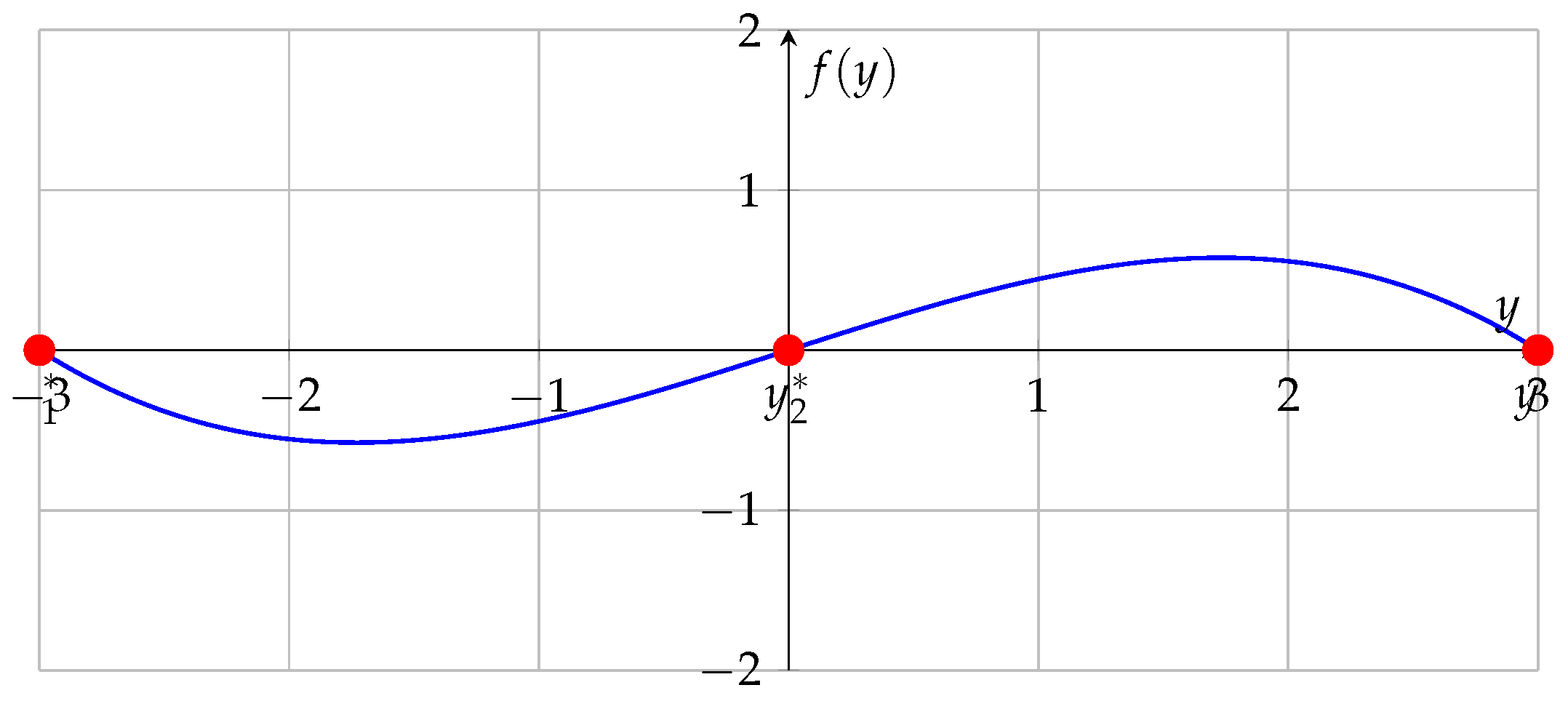
3.1. Autonomous Equations and Phase Line Analysis

For autonomous equations ${\displaystyle \frac{dy}{dt}}=f\left(y\right)$, equilibrium points satisfy $f\left(y^{*}\right)=0$.

Figure 1. Graph of $f\left(y\right)$ showing equilibrium points

Figure 1. Graph of $f\left(y\right)$ showing equilibrium points

3.2. Linear Stability Analysis

For small perturbations $\eta =y-y^{*}$ around equilibrium:

$${\displaystyle \frac{d\eta }{dt}}=f(y^{*}+\eta )\approx f^{\prime }\left(y^{*}\right)\eta$$

Solution: $\eta \left(t\right)={\eta }_0{e}^{f^{\prime }\left(y^{*}\right)t}$.

Stability classification:

• $f^{\prime }\left(y^{*}\right)<0$: asymptotically stable
• $f^{\prime }\left(y^{*}\right)>0$: unstable
• $f^{\prime }\left(y^{*}\right)=0$: linearization inconclusive

3.3. Lyapunov Functions for Nonlinear Stability

For systems where linear analysis fails, Lyapunov’s direct method provides stability criteria.

Definition 1. 

A function $V\left(y\right)$ is a Lyapunov function for equilibrium $y^{*}$ if:

(1)

$V\left(y^{*}\right)=0$ and $V\left(y\right)>0$ for $y\ne y^{*}$

(2)

${\displaystyle \frac{dV}{dt}}=\nabla V·f\left(y\right)\le 0$ near $y^{*}$

Example 3.1: Analyze stability of ${\displaystyle \frac{dy}{dt}}=-y^3$.

Solution: Equilibrium: $y^{*}=0$. Linearization: $f^{\prime }\left(0\right)=0$ (inconclusive). Choose $V\left(y\right)={\displaystyle \frac{1}{2}}{y}^2$. Then:

$${\displaystyle \frac{dV}{dt}}=y{\displaystyle \frac{dy}{dt}}=y(-y^3)=-y^4\le 0$$

Thus $y^{*}=0$ is asymptotically stable.

3.4. Bifurcation Analysis

Bifurcations occur when system behavior changes qualitatively with parameter variation.

Example 3.2: Transcritical bifurcation in ${\displaystyle \frac{dy}{dt}}=ry-y^2$.

Equilibria: $y^{*}=0$ and $y^{*}=r$. Stability:

• For $r<0$: $y^{*}=0$ stable, $y^{*}=r$ unstable
• For $r>0$: $y^{*}=0$ unstable, $y^{*}=r$ stable
• At $r=0$: bifurcation point

4. Canonical Models: Detailed Analysis

4.1. Exponential Growth and Decay

The fundamental model ${\displaystyle \frac{dP}{dt}}=kP$ has solution $P\left(t\right)=P_0{e}^{kt}$.

Applications:

• Population growth ($k>0$)
• Radioactive decay ($k<0$)
• Compound interest (k as interest rate)

Table 2. Half-life and doubling time calculations.

Process	Formula	Example
Half-life	$T_{1/2}={\displaystyle \frac{ln2}{\left|k\right|}}$	Carbon-14: $T_{1/2}=5730$ years
Doubling time	$T_2={\displaystyle \frac{ln2}{k}}$	Bacteria: $T_2=20$ minutes

Table 2. Half-life and doubling time calculations.

Process	Formula	Example
Half-life	$T_{1/2}={\displaystyle \frac{ln2}{\left|k\right|}}$	Carbon-14: $T_{1/2}=5730$ years
Doubling time	$T_2={\displaystyle \frac{ln2}{k}}$	Bacteria: $T_2=20$ minutes

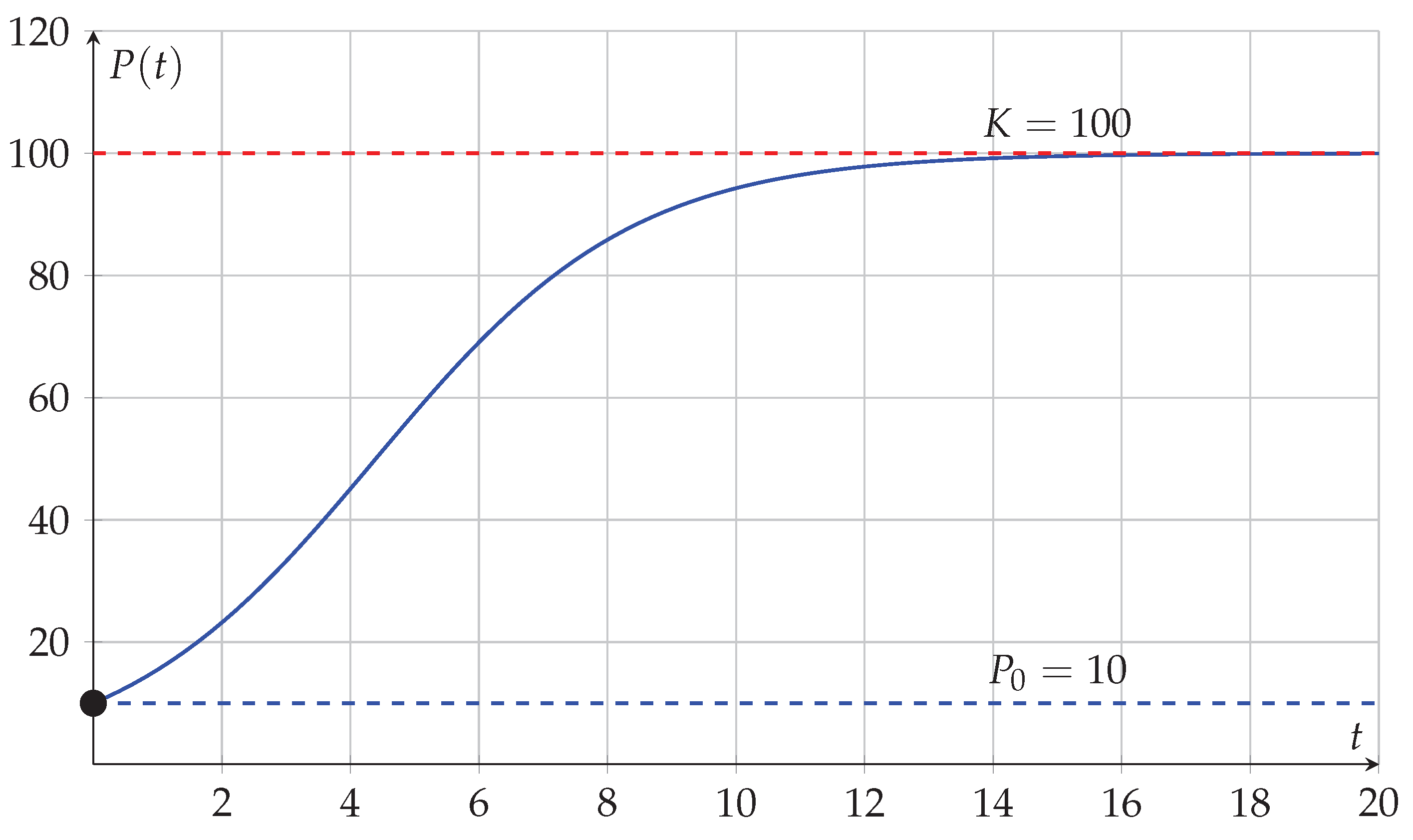
4.2. Logistic Growth: Complete Analysis

The logistic equation:

$${\displaystyle \frac{dP}{dt}}=rP\left(1-{\displaystyle \frac{P}{K}}\right)$$

(4.1)

Analytical solution via separation:

$$P\left(t\right)={\displaystyle \frac{K}{1+\left(\frac{K-P_0}{P_0}\right)e^{-rt}}}$$

(4.2)

Figure 2. Logistic growth with $r=0.5$, $K=100$, $P_0=10$

Figure 2. Logistic growth with $r=0.5$, $K=100$, $P_0=10$

4.3. Newton’s Law of Cooling: Extended Models

General form: ${\displaystyle \frac{dT}{dt}}=-k(T-T_{\mathrm{env}})$. Solution:

$$T\left(t\right)=T_{\mathrm{env}}+(T_0-T_{\mathrm{env}})e^{-kt}$$

Example 4.1: Forensic application. A body found at 2 AM with temperature 27°C. Room temperature 21°C. At 3 AM, temperature is 26°C. Time of death?

Solution: Using two measurements:

$$27=21+(T_0-21)e^{-k·t_1}$$

$$26=21+(T_0-21)e^{-k·(t_1+1)}$$

Dividing: ${\displaystyle \frac{27-21}{26-21}}=e^k\Rightarrow k=ln(6/5)\approx 0.1823$. Assuming body temperature at death = 37°C:

$$27=21+(37-21)e^{-0.1823t_1}\Rightarrow t_1\approx 5.3\mathrm{hours}$$

Death occurred approximately 5.3 hours before 2 AM, around 8:42 PM.

4.4. Gompertz Growth Model

Used for tumor growth modeling:

$${\displaystyle \frac{dP}{dt}}=rPln\left({\displaystyle \frac{K}{P}}\right)$$

(4.3)

Solution: $P\left(t\right)=Kexp\left(ln(P_0/K)e^{-rt}\right)$.

5. Numerical Methods: Algorithms and Implementation

5.1. Euler’s Method: Error Analysis

Forward Euler method:

$$y_{n+1}=y_n+hf(t_n,y_n)$$

(5.1)

Local truncation error: $LTE={\displaystyle \frac{h^2}{2}}{y}^{\prime \prime }\left({\xi }_n\right)=O\left(h^2\right)$. Global error: $|y\left(t_n\right)-y_n|\le {\displaystyle \frac{hM}{2L}}(e^{L(t_n-t_0)}-1)$, where $M=max|y^{\prime \prime }\left(t\right)|$.

5.2. Runge-Kutta Methods Family

5.2.1. Second-Order Methods (RK2)

• Modified Euler: $y_{n+1}=y_n+hf(t_n+h/2,y_n+{\displaystyle \frac{h}{2}}f(t_n,y_n))$
• Heun’s method: $y_{n+1}=y_n+{\displaystyle \frac{h}{2}}[f(t_n,y_n)+f(t_{n+1},y_n+hf(t_n,y_n))]$

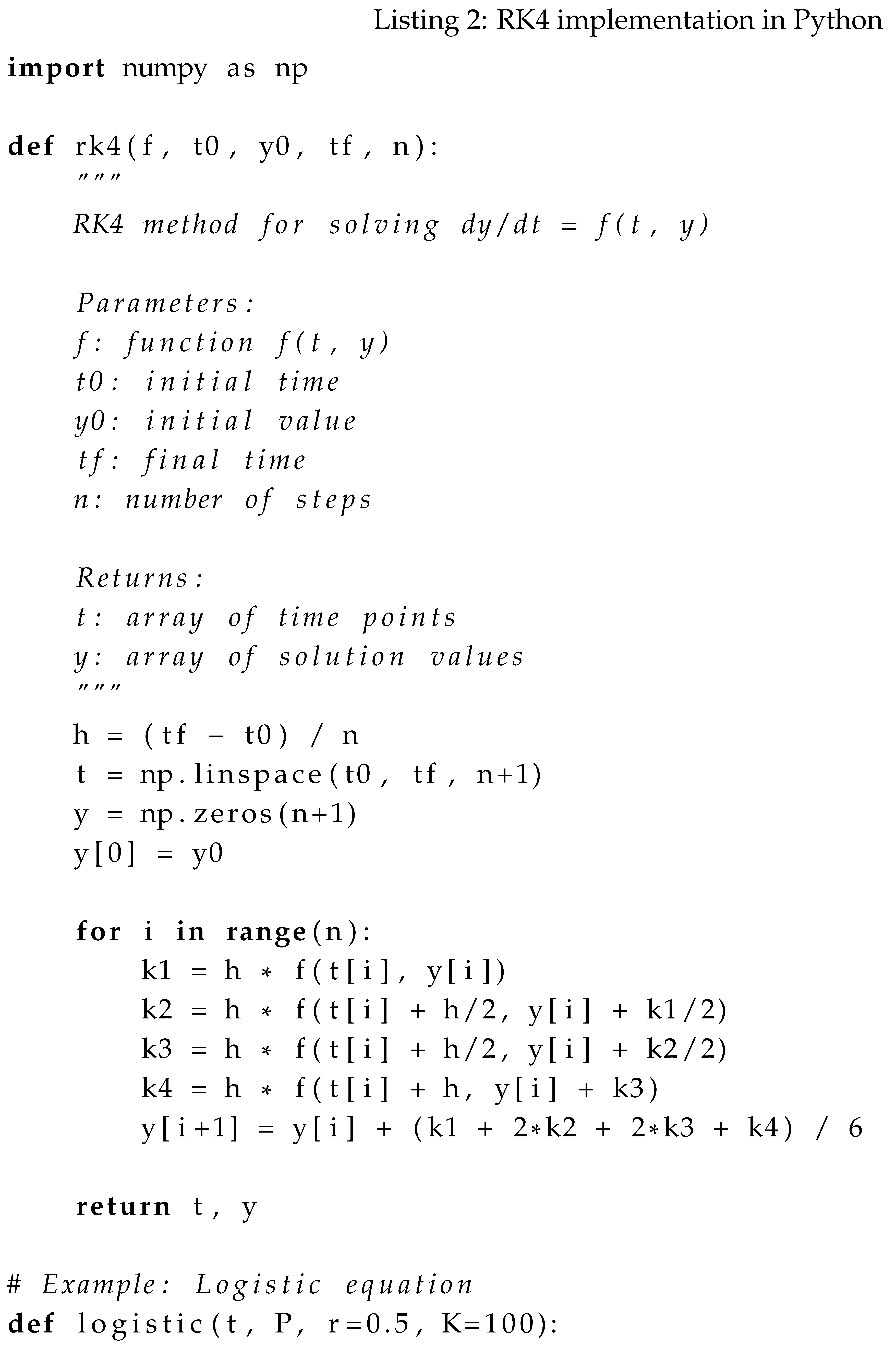
5.2.2. Classical Fourth-Order Runge-Kutta (RK4)

$$\begin{array}{cc}\hfill k_1& =hf(t_n,y_n)\hfill \\ \hfill k_2& =hf(t_n+h/2,y_n+k_1/2)\hfill \\ \hfill k_3& =hf(t_n+h/2,y_n+k_2/2)\hfill \\ \hfill k_4& =hf(t_n+h,y_n+k_3)\hfill \\ \hfill y_{n+1}& =y_n+{\displaystyle \frac{1}{6}}(k_1+2k_2+2k_3+k_4)\hfill \end{array}$$

Local error: $O\left(h^5\right)$, global error: $O\left(h^4\right)$.

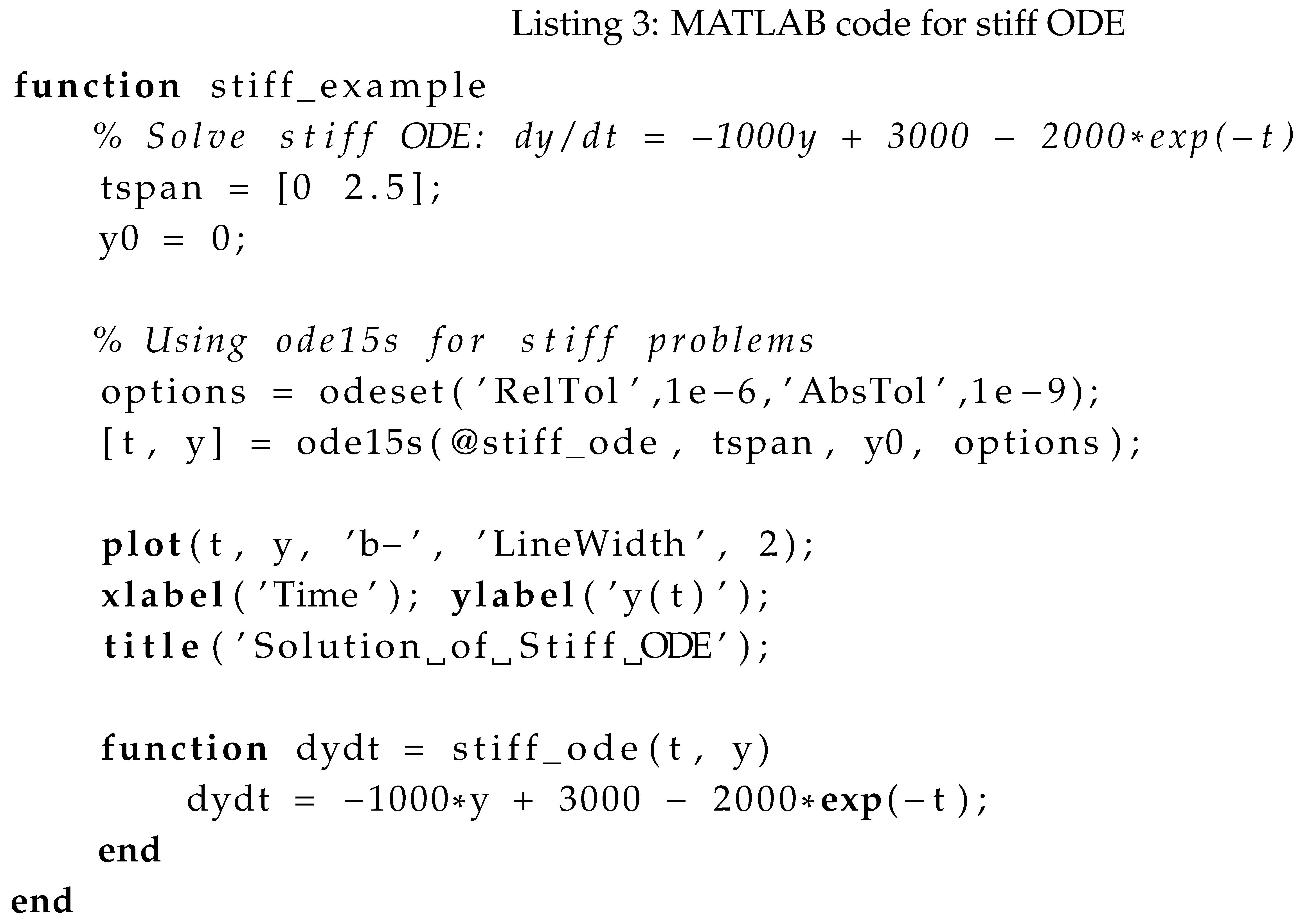
5.3. Stiff Equations and Implicit Methods

For stiff equations like ${\displaystyle \frac{dy}{dt}}=-1000y+3000-2000e^{-t}$, explicit methods require very small h.

5.3.1. Backward Euler Method

$$y_{n+1}=y_n+hf(t_{n+1},y_{n+1})$$

(5.3)

Unconditionally stable but requires solving nonlinear equation.

5.3.2. Trapezoidal Rule (Crank-Nicolson)

$$y_{n+1}=y_n+{\displaystyle \frac{h}{2}}[f(t_n,y_n)+f(t_{n+1},y_{n+1})]$$

(5.4)

Second-order accurate, A-stable.

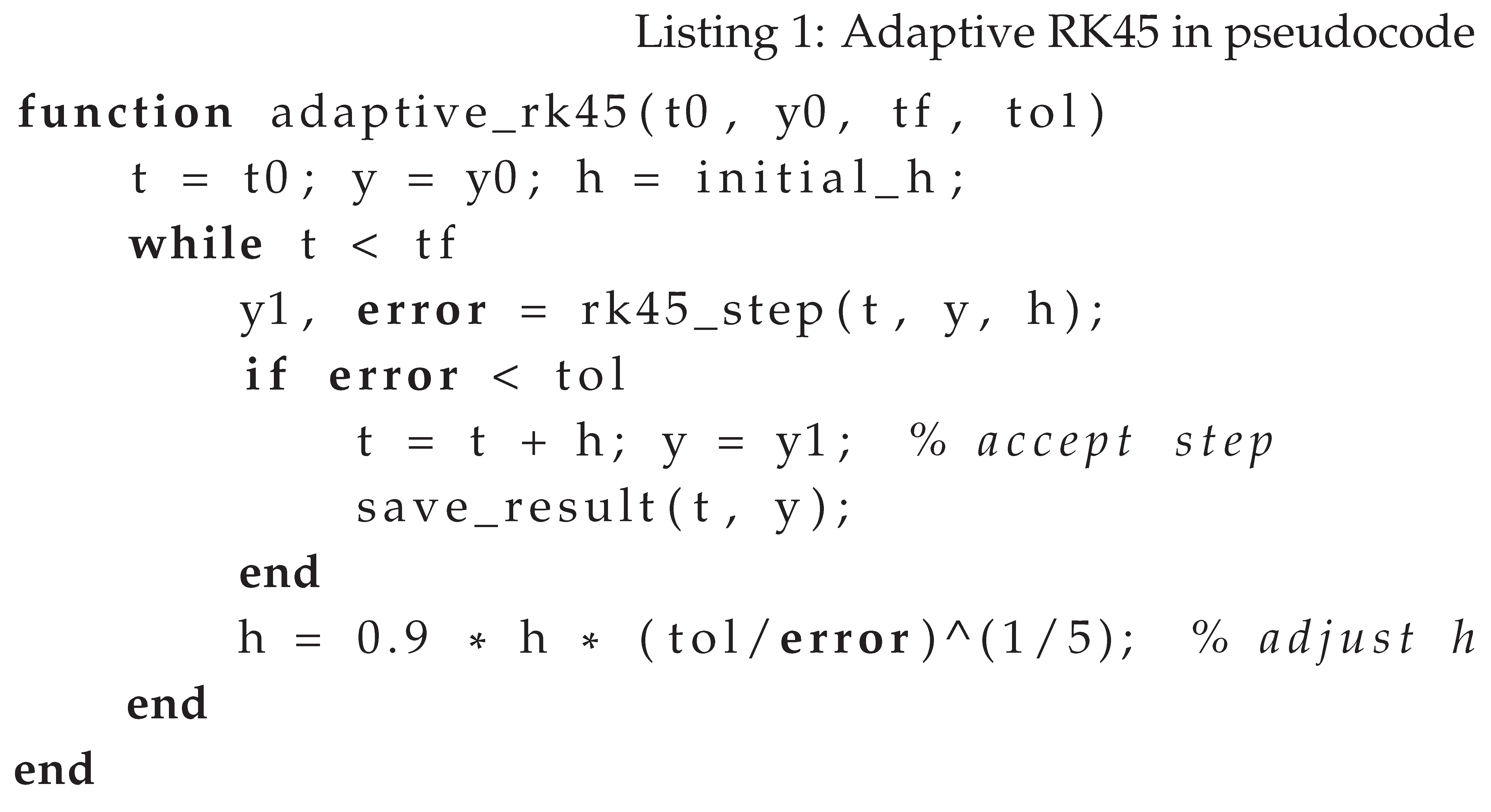
5.4. Adaptive Step Size Control

Step size adjustment based on error estimation:

6. Advanced Topics and Extensions

6.1. Allee Effect Models

Strong Allee effect:

$${\displaystyle \frac{dP}{dt}}=rP\left(1-{\displaystyle \frac{P}{K}}\right)\left({\displaystyle \frac{P}{A}}-1\right),0<A<K$$

(6.1)

Three equilibria: $P^{*}=0$ (stable), $P^{*}=A$ (unstable threshold), $P^{*}=K$ (stable).

6.2. Delay Differential Equations (DDEs)

Include historical dependence: ${\displaystyle \frac{dy}{dt}}=f(t,y\left(t\right),y(t-\tau ))$.

Example: Hutchinson’s delayed logistic equation:

$${\displaystyle \frac{dP}{dt}}=rP\left(t\right)\left(1-{\displaystyle \frac{P(t-\tau )}{K}}\right)$$

(6.2)

Can exhibit oscillatory behavior and stability switches.

6.3. Stochastic Differential Equations (SDEs)

Add random fluctuations: $d{Y}_t=f(t,Y_t)dt+g(t,Y_t)d{W}_t$.

Example: Stochastic logistic growth:

$$dP=rP\left(1-{\displaystyle \frac{P}{K}}\right)dt+\sigma Pd{W}_t$$

(6.3)

6.4. Fractional Differential Equations

Generalize to fractional order: $D^{\alpha }y=f(t,y)$, $0<\alpha \le 1$.

7. Applications Across Disciplines

7.1. Ecology and Population Dynamics

• Lotka-Volterra predator-prey models
• Metapopulation dynamics
• Species invasion models
• Harvesting and management strategies

7.2. Biomedical Sciences

7.2.1. Pharmacokinetics: One-Compartment Model

$${\displaystyle \frac{dC}{dt}}=-{\displaystyle \frac{CL}{V}}C+{\displaystyle \frac{R\left(t\right)}{V}},C\left(0\right)=C_0$$

(7.1)

where C = concentration, $CL$ = clearance, V = volume, $R\left(t\right)$ = infusion rate.

7.2.2. Epidemiology: SI Model

$${\displaystyle \frac{dS}{dt}}=-\beta SI,{\displaystyle \frac{dI}{dt}}=\beta SI-\gamma I$$

(7.2)

Basic reproduction number: $R_0={\displaystyle \frac{\beta S_0}{\gamma }}$.

7.3. Physics and Engineering

7.3.1. Electrical Circuits

RC circuit: ${\displaystyle \frac{dV}{dt}}=-{\displaystyle \frac{1}{RC}}V+{\displaystyle \frac{1}{C}}I\left(t\right)$. RL circuit: ${\displaystyle \frac{dI}{dt}}=-{\displaystyle \frac{R}{L}}I+{\displaystyle \frac{1}{L}}V\left(t\right)$.

7.3.2. Mechanics with Drag

$$m{\displaystyle \frac{dv}{dt}}=mg-kv-c{v}^2$$

(7.3)

Linear drag ($c{v}^2=0$): $v\left(t\right)={\displaystyle \frac{mg}{k}}(1-e^{-kt/m})$. Quadratic drag: analytical solution involves hyperbolic functions.

7.4. Economics and Finance

7.4.1. Solow Growth Model

$${\displaystyle \frac{dk}{dt}}=sf\left(k\right)-(n+\delta )k$$

(7.4)

where k = capital per worker, s = savings rate, n = population growth, $\delta$ = depreciation.

8. Computational Implementation Examples

8.1. Python Implementation of RK4

8.2. MATLAB Implementation for Stiff Problems

9. Conclusions and Future Directions

First-order ODEs continue to be indispensable in scientific modeling. Future directions include:

• Machine Learning Integration: Neural ODEs that parameterize $f(t,y)$ with neural networks
• High-Dimensional Systems: Applications in data science and network dynamics
• Stochastic Methods: Improved numerical methods for SDEs
• Hybrid Systems: Combining continuous ODEs with discrete events
• Uncertainty Quantification: Propagating parameter uncertainties through ODE models

The interplay between analytical insight and computational power continues to drive innovation in both theoretical understanding and practical applications of first-order differential equations.

Appendix A.1. Common Integrals

$$\begin{array}{cc}\hfill \int {\displaystyle \frac{dx}{x}}& =ln\left|x\right|+C\hfill \\ \hfill \int {\displaystyle \frac{dx}{a^2+x^2}}& ={\displaystyle \frac{1}{a}}arctan\left({\displaystyle \frac{x}{a}}\right)+C\hfill \\ \hfill \int {\displaystyle \frac{dx}{a^2-x^2}}& ={\displaystyle \frac{1}{2a}}ln\left|{\displaystyle \frac{a+x}{a-x}}\right|+C\left(\right|x|\ne a)\hfill \\ \hfill \int {\displaystyle \frac{dx}{\sqrt{a^2-x^2}}}& =arcsin\left({\displaystyle \frac{x}{a}}\right)+C\left(\right|x|<a)\hfill \end{array}$$

Appendix A.2. Integration by Parts Formula

$$\int udv=uv-\int vdu$$

References

- Brauer, F.; Castillo-Chavez, C. Mathematical Models in Population Biology and Epidemiology; Springer Science & Business Media, 2012. [Google Scholar]
- Hirsch, M. W.; Smale, S.; Devaney, R. L. Differential Equations, Dynamical Systems, and an Introduction to Chaos; Academic Press, 2012. [Google Scholar]
- Strogatz, S. H. Nonlinear Dynamics and Chaos: With Applications to Physics, Biology, Chemistry, and Engineering; CRC Press, 2018. [Google Scholar]
- Trench, W. F. Elementary Differential Equations with Boundary Value Problems; Trinity University, 2013. [Google Scholar]
- Boyce, W. E.; DiPrima, R. C.; Meade, D. B. Elementary Differential Equations and Boundary Value Problems; John Wiley & Sons, 2012. [Google Scholar]
- Butcher, J. C. Numerical Methods for Ordinary Differential Equations; John Wiley & Sons, 2016. [Google Scholar]
- Ascher, U. M.; Petzold, L. R. Computer Methods for Ordinary Differential Equations and Differential-Algebraic Equations; SIAM, 1998. [Google Scholar]
- Edelstein-Keshet, L. Mathematical Models in Biology; SIAM, 2005. [Google Scholar]
- Murray, J. D. Mathematical Biology: I. An Introduction; Springer, 2002. [Google Scholar]
- Kloeden, P. E.; Platen, E. Numerical Solution of Stochastic Differential Equations; Springer, 2011. [Google Scholar]
- Hale, J. K.; Kocak, H. Dynamics and Bifurcations; Springer Science & Business Media, 2012. [Google Scholar]
- Chen, W.; Holm, S. Fractional Derivative Modeling in Mechanics and Engineering; Springer, 2014. [Google Scholar]
- Shampine, L. F. Numerical Solution of Ordinary Differential Equations; Chapman and Hall, 1997. [Google Scholar]
- Keshava, R. Ordinary Differential Equations: Principles and Applications; Tata McGraw-Hill, 1967. [Google Scholar]
- Arnold, V. I. Ordinary Differential Equations; Springer, 1992. [Google Scholar]
- Coddington, E. A.; Levinson, N. Theory of Ordinary Differential Equations; McGraw-Hill, 1955. [Google Scholar]
- Hartman, P. Ordinary Differential Equations; SIAM, 2002. [Google Scholar]
- Hale, J. K. Ordinary Differential Equations; Krieger Publishing Company, 1980. [Google Scholar]
Disclaimer/Publisher’s Note: The statements, opinions and data contained in all publications are solely those of the individual author(s) and contributor(s) and not of MDPI and/or the editor(s). MDPI and/or the editor(s) disclaim responsibility for any injury to people or property resulting from any ideas, methods, instructions or products referred to in the content. |
© 2025 by the authors. Licensee MDPI, Basel, Switzerland. This article is an open access article distributed under the terms and conditions of the Creative Commons Attribution (CC BY) license (http://creativecommons.org/licenses/by/4.0/).
Copyright: This open access article is published under a Creative Commons CC BY 4.0 license, which permit the free download, distribution, and reuse, provided that the author and preprint are cited in any reuse.