
Submitted:
25 December 2025
Posted:
26 December 2025
You are already at the latest version
Abstract
Lung cancer remains one of the leading causes of cancer-related mortality worldwide, highlighting the importance of early detection for improving patient survival rates. However, current machine learning approaches for lung cancer prediction often depend on suboptimal model configurations, limited systematic ensemble comparisons, and insufficient interpretability. This study introduces a novel framework, called Lung Explainable Ensemble Optimizer (LungEEO), that integrates three methodological advances: (1) comprehensive hyperparameter optimization across 50 configurations of nine machine learning algorithms for base model selection, (2) a systematic comparison of Hybrid Majority Voting strategies, including unweighted hard voting, weighted hard voting, and soft voting with an ensemble stacking approach, and (3) a dual explainable AI (XAI) layer based on SHAP and LIME to provide parallel global and local explanations. Experiments conducted on two heterogeneous lung cancer datasets indicate that ensemble approaches consistently outperform individual models. Weighted hard voting achieved the best performance on Dataset 1 (Accuracy: 89.04%, F1-Score: 89.04%), whereas ensemble stacking produced superior outcomes on Dataset 2 (Accuracy: 87.95%, F1-Score: 87.95%). Following extensive hyperparameter tuning, Random Forest and Multi-Layer Perceptron performed consistently well as base learners on both datasets. In addition, integrating SHAP with LIME offers additional insights into model behavior, boosting the interpretability of ensemble predictions, and strengthening their potential clinical applicability. To the best of our knowledge, the combined use of these interpretability techniques within an ensemble framework has received limited attention in existing lung cancer prediction studies. Overall, the proposed LungEEO framework offers a promising balance between predictive performance and interpretability, supporting its potential use in clinical decision support.
Keywords:
lung cancer
; tabular data
; machine learning
; classification
; confusion matrix
; heat map
1. Introduction
Lung cancer remains one of the leading causes of cancer-related mortality worldwide, exceeding many other major cancers in terms of annual death rates [1,2]. Despite developments in treatment strategies, patient survival remains highly dependent on early-stage diagnosis. Factors such as increasing air pollution, smoking habits, occupational exposure, and lifestyle-related risks have contributed to a steady rise in lung cancer incidence over the last few decades. In recognition of these challenges, United Nations Sustainable Development Goal (SDG) 3.9 highlights the urgent need to reduce mortality associated with hazardous environmental pollution [3]. From a clinical perspective, early-stage lung cancer frequently appears through nonspecific symptoms, including shortness of breath, persistent cough, fatigue, and back pain, potentially leading to delays in diagnosis and suboptimal treatment outcomes [4].
Traditional diagnostic approaches, including imaging and biopsies, often detect lung cancer at advanced stages, thereby limiting available therapy options. In recent years, machine learning (ML) techniques have demonstrated significant potential for earlier lung cancer detection through the automated analysis of structured tabular data, such as demographic characteristics, clinical measurements, lifestyle factors, symptoms, comorbidities, and treatment-related variables [5,6]. These data-driven techniques make predictive modeling more scalable and cost-effective, particularly in resource-constrained healthcare settings.
Despite these advances, several significant challenges remain insufficiently addressed in the existing lung cancer prediction literature. First, many studies apply limited hyperparameter optimization, which can result in suboptimal base model performance. Second, ensemble learning strategies are often evaluated in isolation, without the systematic comparison of different voting mechanisms and stacking approaches within a unified experimental framework. Third, and most important for clinical adoption, model interpretability is frequently overlooked, with many high-performing models acting as black boxes, providing no insight into the causes underlying their predictions.
Explainable Artificial Intelligence (XAI) approaches have become increasingly significant for addressing the interpretability gap in predictive models. Model-agnostic techniques, such as SHapley Additive exPlanations (SHAP) and Local Interpretable Model-agnostic Explanations (LIME), provide additional insights by offering global feature importance and instance-level explanations, respectively. Although these techniques have been applied independently in healthcare research, their combined and systematic use inside ensemble-based lung cancer prediction frameworks remains limited, particularly for investigating ensemble behavior across diverse patient profiles.
Ensemble learning methods, including majority hard voting, majority soft voting, weighted hard voting, and ensemble stacking, have demonstrated potential for enhancing predictive robustness by combining heterogeneous base classifiers [7]. However, present research rarely provides a comprehensive evaluation that integrates exhaustive base-model optimization, different ensemble techniques, and parallel explainable AI (XAI) analysis, especially when applied to newly curated datasets. Furthermore, most of the previous the work is based on well-established benchmark datasets that have been thoroughly examined, which may limit the assessment of model generalizability.
To address these gaps, this study presents a unified and interpretable ensemble framework known as the Lung Explainable Ensemble Optimizer (LungEEO). The framework is evaluated using two newly curated lung cancer tabular datasets for which no existing state-of-the-art benchmarks or systematic ensemble analyses are currently available. This experimental setting allows for a fair and unbiased assessment of model evaluation while establishing baseline results for future research. Accordingly, this study aims to address the following critical research questions:
- Which optimized individual machine learning models provide the most reliable performance for early lung cancer prediction from structured tabular data?
- How do different Hybrid Majority Voting strategies compare with Ensemble Stacking in terms of predictive accuracy and robustness?
- How can the combined use of SHAP and LIME enhance the interpretability and clinical reliability of both base learners and ensemble models?
The main contribution of this work is threefold:
- An exhaustive base-model optimization strategy, involving 50 hyperparameter configurations across nine heterogeneous machine learning algorithms which ensures robust model selection and maximizes ensemble diversity.
- A comprehensive ensemble learning framework that systematically compares Hybrid Majority Voting strategies (unweighted hard voting, weighted hard voting, and soft voting) with Ensemble Stacking for lung cancer prediction using structured tabular data.
- A dual XAI-driven interpretability analysis, jointly applying SHAP and LIME to both base and ensemble models to provide additional global and local explanations, thereby enhancing transparency and supporting potential clinical adoption.
The organization of the paper is as follows: Section 2 describes related works; Section 3 describes the methodology of this Study; Section 4 describes the Results and Evaluation of the proposed methods; Section 5 describes the discussion; Section 6 stands for the Conclusions and Future works; Section illustrates the Statements and Declarations; Section represents the abbreviations.
2. Related Works
Nitha and Vinod Chandra [8] proposed a explainable machine learning framework aimed at predicting lung cancer in relation to the impact of pesticide exposure. Using three datasets – the Thai Dataset (680 instances), Lung cancer Prediction Dataset (1000 Samples), and a Survey Lung cancer Dataset (309 Patients) – the study focused on numerical attributes such as pesticide exposure, duration, age, occupation, symptoms like coughing blood, smoking history. Various machine learning models such as XGBoost, Logistic Regression, Decision Tree, Gaussian Naïve Bayes, Multi-Layer Perceptron, Random Fores, Support Vector Machine (SVM) was used that delivered superior performance. Two Stage Feature Selection methods such as Extra Tree Classifier and PCA for Dimensionality Reduction were applied. XGBoost with SMOTE combined with ENN (Edited Nearest Neighbour) with PCA Preprocessing performed the best results, achieving 99% accuracy in all of the datasets. Despite its high performance the study acknowledged its limitations such as overfitting risks due to high-dimensional data. Future directions suggested validating models on larger multi-omics data and developing real-time risk monitoring tools, investigating deep learning approaches for further accuracy enhancement.
Maurya et al. [6] conducted an experiment to study the comparative performance of various machine learning algorithms for lung cancer prediction. The study used public datasets from Kaggle Comprising of 310 samples capturing data such as patient’s habits (e.g., smoking, alcohol consumption) and symptoms (e.g., yellow fingers, chest pain, anxiety). The features also included demographic details alongside clinical symptoms. Multiple machine learning models such as Logistic Regression, Gaussian Naïve Bayes, Bernoulli Naïve Bayes, SVM, Random Forest, K-Nearest Neighbours (KNN), Extreme Gradient Boosting (XGB), Extra Trees, AdaBoost and ensemble methods combining XGB and AdaBoost, as well as a Multi-Layer Perceptron (MLP). The data preprocessing steps involved removing duplicate entries, splitting the data into 80:20 ratio for training and testing and performing 10-fold cross validation. KNN Achieved the highest accuracy achieving an accuracy of 92.86% followed closely by Bernoulli Naïve Bayes and Gaussian Naïve Bayes. Persons Correlation heat maps were also used for feature correlation analysis. Some limitations of the study were the usage of a very small dataset, and using only one ensemble technique and not exploring the other techniques such as bagging, stacking etc.
Zheng et al. [9] developed a machine learning framework using XGBoost for the classification of Benign Malignant pulmonary nodules based on low-dose spiral computerized tomography (LDCT) and clinical data from Screening. The study utilized two datasets, the primary dataset was collected from physical examination data from the Institute of Health management of the General Hospital of the Chinese People’s Liberation Army (PLA) which container 1335,503 participants and an external validation dataset was collected from the Henan Provincial People’s Medical Health Examination Centre and Sichuan Provincial People’s Hospital which contained 5.146 participants. Both demographic data and Clinical Data were collected for the experiment. The top 15 clinical features were selected via XGBoost feature importance ranking. Processing involved encoding the categorical Data’s, Splitting the data in 80:20 ration for training and testing, hyperparameter tuning through grid search and automatic handling of missing data using XGBoost. The model achieved an AUC of 0.76 and an accuracy of 0.75 in internal validation, and an improved AUC of 0.87 an accuracy of 0.80 in external validation. Although achieving good results, some limitations of the study included using limited number of data samples which limited generalizability and also, usage of only one type of Ensemble technique (The other ensemble technique could potentially improve performance of the models).
Wani er al. [10] proposed DeepXplainer, an interpretable deep-learning based framework for lung cancer prognosis. The study used a Lung Cancer Survey Dataset containing 309 patient records. The dataset included clinical attributes such as coughing, shortness of breath, and chest pain, among others. Several machine learning models were explored such as Convolutional Neural Network (CNN), XGBoost, Naïve Bayes, Random Forest, and CATBoost. The proposed hybrid ConvXGB model combined CNN for automated feature learning with XGBoost for final classification. Data preprocessing involved label encoding, duplicate removal, 80-20 train-test splitting, MinMaxScaler normalization, and label binarization. The ConvXGB model achieved 97.43% accuracy, 98.71% sensitivity, and 98.08% F1-score. Model interpretability was done using SHAP (Shapley Additive exPlanations) for both local and global predictions. Some limitations of this paper included not exploring more diverse datasets, comparison with other ensemble techniques.
Lei et al. [11] conducted a study based on nomogram-based and machine learning-based methods for survival prediction of non-small cell lung cancer (NSCLC) patients. The authors used a dataset that contained 6,586 patients from the Cancer Hospital Affiliated to Chongqing University (CUCH), China. The dataset included clinical, pathological, demographic, and treatment-related features such as age, sex, weight, smoking history, Tumour Staging, and treatment modalities. Several Machine Learning Algorithm was implemented such as Logistic Regression, Random Forest, XGBoost, Decision Tree, and Light Gradient Boosting Machine. Feature selection was done using pairwise Spearman’s rank correlation and the Boruta Method. Among the models Random Forest performed the best across multiple points suggesting it’s reliability for long-term survival prediction. Limitations of the study included lack of external validation and potential improvement to model’s using different ensemble techniques. Rule-based knowledge could also be integrated to enhance the predictions of the machine learning models.
Dritsas and Trigka [12] developed machine learning models using publicly available Kaggle dataset containing 309 patients for Lung Cancer Prediction. The dataset contained variety of demographic and clinical feature such as coughing, shortness of breath, chest pain and other health indicators such as chronic diseases and allergy history. A wide range of machine learning models were explored such as Naïve Bayes (NB), Bayesian Network, Stochastic Gradient Descent, Support Vector Machine (SVM), Logistic Regression (LR), Random Forest (RF), Random Tree (RT), Reduced Error Pruning Tree (RepTree), Rotation Forest (RotF), and AdaBoostM1. Feature selections were done using Gain Ratio and Random Forest rankings. SMOTE was also applied for class balancing in the data. Rotation Forest achieved the best accuracy of 97.1% with an AUC of 99.3%. Some limitations of the study noted by the authors were the non-generalizability of the models, and non-clinical features of the dataset. Future work also included using deep learning techniques such as LSTM and CNN.
Chandasekar et al. [13] proposed a novel multivariate boosting classification method name Multivariate Ruzicka Regressed eXtreme Gradient Boosting Data Classification (MRRXGBDC). The authors used four datasets: The Lung cancer dataset (1000 instances), the Thoracic Surgery dataset (470 instances), the Air Quality Lung cancer dataset (2602 countries), and the Lung 16 lung cancer dataset (551, 065 instances). All of the datasets were publicly available. The dataset contained features such as ID, age, gender, air pollution exposure, alcohol use, dust allergy, and occupational hazards. One of the unique features of the proposed model was its ability to handle missing values and handle imbalanced data. Limitations identified for this study includes only exploring only one form of Ensemble technique, reducing computational complexity and improving generalizability of the disease prediction system.
Wang et al. [14] conducted the machine learning based study on the investigation of gender-specific prognosis in lung cancer patients for the Surveillance, Epidemiology and SEER database comprising of 28,458 cases. A range of machine learning models such as Naïve Bayes, Decision Trees, Random Forest, Extreme Gradient Boosting, K-Nearest Neighbour, Logistic Regression, and Support Vector Machine with Random Forest achieving the best overall performance. For one-year survival XGB model achieved 90.75% accuracy, for three-year survival prediction LR achieved the best accuracy of 75.65% accuracy, and for Five-year Survival prediction LR again achieved the best accuracy getting about 71.79% accuracy. Major limitations of the study was the restricted scope of clinical features in the SEER database, major features were absent such as smoking and drinking history. Also, the comparison the other ensemble methods such as hard bagging, stacking and soft voting were not explored in this study.
Cui et al. [15] explored machine learning approaches for predicting early death among lung cancer patients with bone metastases. Using the SEER database the study utilized demographic and clinical characteristics of the patients to be used as predictive features. Logistic Regression, Extreme Gradient Boosting, Random Forest, Neural Network, Gradient Boosting Machine were applied for comparative studies. Gradient Boosting Machine performed the best among the other machine learning models. To interpret the results. Local Interpretable Model-agnostic Explanations (LIME) and Shapley Additive exPlanations (SHAP) were employed. Some of the limitations of this study were lack of certain clinical predictors such as the quantity and specific location of the bone metastases, and the absence of external validation sets.
Doppalupudi et al. [16] investigated deep learning based approaches for predicting lung cancer survival periods using the SEER database. The dataset included both categorical and quantitative variables such age, number of tumours, chemotherapy status, and AJCC TNM Staging factors. Several machine learning and deep learning models were applied, such as Artificial Neural, Convolutional Neural Network, Recurrent Neural Network, Random Forest, Support Vector Machine, Naïve Byes, Gradient Boosting Machines and Linear Regression for comparative analysis. A custom ensemble was also developed, which was based on stacking. Feature selection was done using LASSO regression. ANN performed the best for classification task with an accuracy of 71.18% and CNN was the most effective for regressions tasks achieving 13.50% RMSE and 50.66% R2. Some limitations of the study were the data included imbalanced dataset and higher error rates for predicting longer survival periods.
Although existing studies have demonstrated the effectiveness of machine learning, ensemble methods, and explainable artificial intelligence (XAI) techniques for lung cancer prediction, several important gaps remain. Many prior works consider a limited set of classifiers or evaluate a single ensemble strategy, without systematically comparing multiple voting and stacking mechanisms within a unified framework. In addition, hyperparameter optimization is often constrained, which may limit both base-model performance and ensemble diversity.
Moreover, explainability techniques such as SHapley Additive exPlanations (SHAP) and Local Interpretable Model-agnostic Explanations (LIME) are typically applied independently and primarily to individual models, with limited focus on their combined use for interpreting ensemble behavior. Finally, the majority of existing studies rely on well-established benchmark datasets, which restricts the assessment of model generalizability and limits the availability of baseline results for newly curated data.
Motivated by these limitations, this study proposes the Lung Explainable Ensemble Optimizer (LungEEO), a unified framework that integrates exhaustive base-model optimization, systematic evaluation of multiple ensemble learning strategies, and a dual XAI analysis using SHAP and LIME. Experiments are conducted on two newly curated lung cancer tabular datasets for which no established state-of-the-art benchmarks currently exist. This evaluation setting enables the establishment of reliable performance baselines while enhancing model interpretability and supporting clinical relevance.
3. Methodology
The proposed study methodology for lung cancer prediction pipeline is illustrated in Figure 1. The following section outlines the methodology of the study which includes the steps taken for data collection, processing and evaluation, creation of machine learning pool for selecting the best machine learning models, constructing ensemble models from the best machine learning model and evaluation. Detailed explanations of the steps of the approaches are as follows.
3.1. Experimental Setup
The Experimental setup for this study was conducted in a Local Machine that used Python 3.11.4 as a runtime environment. The Local Machine used Ryzen 1600 with 6 Core and 12 Threads CPU, 16GB of Ram, and an RTX 3060 12GB of GPU which was used for efficient training of the models. Pandas, Seaborn, and Scikit Learn were used for Data Preprocessing and Splitting, Scaling, and model creation. Imbalanced Learn was used for Over Sampling of the data. Matplotlib was used to visualize the training curves, evaluate the models and create confusion matrices. This setup allowed for efficient and effective experimentation with no compute unit constraints.
3.2. Dataset Description
The datasets were collected from Kaggle [17,18]. A description of the dataset is given in Figure 1. Dataset 1 consisted of 5000 Patient records with 18 features whereas Dataset 2 consists of 20000 records with 16 attributes. Both the dataset includes demographic information such as medical history, lifestyles and symptoms associated with pulmonary disease. The dataset before processing was analysed statistically for null values and if it contained any outliers.

Table 1.
Dataset Description.
| Dataset Name | Attribute | Values | Statistics | ||||||
| Count | Mean | Std | Min | 50% | 75% | Max | |||
| Dataset 1 (lung_cancer_dataset) |
AGE | Numeric Value | 5000 | 57.22 | 0.50 | 30 | 57 | 71 | 84 |
| GENDER | 1 [Female], 0 [Male] | 0.50 | 0.50 | 0 | 1 | 1 | 1 | ||
| SMOKING | 1 [Yes], 0 [No] | 0.66 | 0.47 | 0 | 1 | 1 | 1 | ||
| FINGER_DISCOLORATION | 1 [Yes], 0 [No] | 0.60 | 0.48 | 0 | 1 | 1 | 1 | ||
| MENTAL_STRESS | 1 [Yes], 0 [No] | 0.53 | 0.49 | 0 | 1 | 1 | 1 | ||
| EXPOSURE_TO_POLLUTION | 1 [Yes], 0 [No] | 0.51 | 0.499 | 0 | 1 | 1 | 1 | ||
| LONG_TERM_ILLNESS | 1 [Yes], 0 [No] | 0.43 | 0.49 | 0 | 0 | 1 | 1 | ||
| ENERGY_LEVEL | Numeric Value | 55.03 | 7.91 | 23.25 | 55.05 | 60.32 | 83.04 | ||
| IMMUNE_WEAKNESS | 1 [Yes], 0 [No] | 0.39 | 0.48 | 0 | 0 | 1 | 1 | ||
| BREATHING_ISSUE | 1 [Yes], 0 [No] | 0.80 | 0.39 | 0 | 1 | 1 | 1 | ||
| ALCOHOL_CONSUMPTION | 1 [Yes], 0 [No] | 0.35 | 0.47 | 0 | 0 | 1 | 1 | ||
| THROAT_DISCOMFORT | 1 [Yes], 0 [No] | 0.69 | 0.45 | 0 | 1 | 1 | 1 | ||
| OXYGEN_SATURATION | Numeric Value | 94.99 | 1.48 | 89.92 | 94.97 | 95.98 | 99.79 | ||
| CHEST_TIGHTNESS | 1 [Yes], 0 [No] | 0.60 | 0.48 | 0 | 1 | 1 | 1 | ||
| FAMILY_HISTORY | 1 [Yes], 0 [No] | 0.30 | 0.45 | 0 | 0 | 1 | 1 | ||
| SMOKING_FAMILY_HISTORY | 1 [Yes], 0 [No] | 0.20 | 0.40 | 0 | 0 | 0 | 1 | ||
| STRESS_IMMUNE | 1 [Yes], 0 [No] | 0.20 | 0.40 | 0 | 0 | 0 | 1 | ||
| PULMONARY_DISEASE | 1 [Yes], 0 [No] | Null | Null | Null | Null | Null | Null | ||
| Dataset 2 (lcs_synthetic_20000) |
GENDER | M [Male], F [Female] | 20000 | Null | Null | Null | Null | Null | Null |
| AGE | Numeric Value | 62.20 | 8.20 | 30.00 | 62.00 | 68.00 | 87.00 | ||
| SMOKING | 2 [Yes], 1 [No] | 1.56 | 0.49 | 1.00 | 2 | 2 | 2 | ||
| YELLOW_FINGERS | 2 [Yes], 1 [No] | 1.57 | 0.49 | 1 | 2 | 2 | 2 | ||
| ANXIETY | 2 [Yes], 1 [No] | 1.53 | 0.49 | 1 | 2 | 2 | 2 | ||
| PEER_PRESSURE | 2 [Yes], 1 [No] | 1.50 | 0.50 | 1 | 2 | 2 | 2 | ||
| CHRONIC DISEASE | 2 [Yes], 1 [No] | 1.50 | 0.49 | 1 | 2 | 2 | 2 | ||
| FATIGUE | 2 [Yes], 1 [No] | 1.67 | 0.47 | 1 | 2 | 2 | 2 | ||
| ALLERGY | 2 [Yes], 1 [No] | 1.56 | 0.50 | 1 | 2 | 2 | 2 | ||
| WHEEZING | 2 [Yes], 1 [No] | 1.55 | 0.49 | 1 | 2 | 2 | 2 | ||
| ALCOHOL CONSUMING | 2 [Yes], 1 [No] | 1.55 | 0.49 | 1 | 2 | 2 | 2 | ||
| COUGHING | 2 [Yes], 1 [No] | 1.57 | 0.49 | 1 | 2 | 2 | 2 | ||
| SHORTNESS OF BREATH | 2 [Yes], 1 [No] | 1.64 | 0.47 | 1 | 2 | 2 | 2 | ||
| SWALLOWING DIFFICULTY | 2 [Yes], 1 [No] | 1.47 | 0.49 | 1 | 1 | 2 | 2 | ||
| CHEST PAIN | 2 [Yes], 1 [No] | 1.55 | 0.49 | 1 | 2 | 2 | 2 | ||
| LUNG_CANCER | YES, NO | Null | Null | Null | Null | Null | Null | ||
Pearson Correlation heatmap was also plotted which is provided in Figure 2 to assess the importance of different attributes among each other. The left side of the figure refers to the dataset 1 and right side to the dataset 2. For dataset 1 strong correlations are observed between stress immune and immune weakness, as well as, mental stress and stress immune. For dataset 2, the dataset focuses more on diagnosis-specific features such as yellow fingers, chronic disease etc. The correlations can be seen as weak which allows the machine learning model to learn from the data independently and evaluate feature contributions automatically.
3.2.1. Data Pre-Processing
Preprocessing is crucial step in any machine learning experiment. It prepares the data to be fed inside the machine learning model.
A class-based count was measured to check class imbalance which is shown in Figure 3. As there was imbalance between the classes which could potentially make the machine learning model biased. Synthetic Minority Oversampling (SMOTE) was applied to balance the classes. The data was split into two sets for training (80%) and testing (20%). A standard scaling was applied to normalize the data. It transforms the data in such a way that the data has a mean of zero and a standard deviation of 1.
3.2.2. Base Learner Pool and Hyperparameter Optimization
After preprocessing a comprehensive set of machine learning classifiers were selected for the detection of Lung Cancer from the tabular dataset. A pool of 9 machine learning models were created with 50 different hyperparameters settings by fine tuning. The hyperparameters of the models are given in Table 2. The hyperparameters were selected based on a discrete search space of the nine candidate algorithms covering regularization strengths and for logistic regression, estimator counts and feature sampling strategies for Random Forest and boosting methods. These choices were informed by standard practice in the literature and preliminary experiments. A grid-styled sweep was performed over the combination of these parameters on the training data to guard against overfitting and ensure balanced performance. This exhaustive tuning of the models helped identify the strongest base learners and created the performance diversity necessary for a robust ensemble creation.
-
Logistic Regression: Logistic Regression supervised machine learning model which is used widely binary classification problems. It uses the logistic (Sigmoid) function to map the linear combination of input features into probability values ranging from 0 to 1.The probability indicates the likelihood of that given input corresponds to one of the predefined classes. In this study Logistic Regression is used due to its simplicity, interpretability and effectiveness.
- K-Nearest Neighbour: K-Nearest Neighbour is a non-parametric supervised machine learning model. The main methodology behind this classifier is that it classifies an object based on the plurality vote by its neighbour. The neighbours to be considered or k, and the distant metric to be used in the voting is considered as a hyperparameter. KNN was introduced in this study for its robustness and its classification performance which it does without making any assumptions about the data distribution.
-
Naïve Bayes: Naïve Bayes is a simple classifier that assigns probabilities to different labels from the vector of feature values. It is based on the Bayes Theorem.It calculates the posterior probability of each class based on the input features and selects the class with the highest probability. Despite, its complexity it often performs well in high dimensional dataset. This model was added to the study to analyse the benchmark of probabilistic modelling.
- Support Vector Machine: Support Vector Machine or otherwise known as SVM is a supervised max-margin model that can be used for both classification and regression analysis. It tries the find the optimal hyperplane that separates the different classes by maximizing the margin of difference between them. It can handle both linear and non-linear input features. For non-linear input features it uses different kernel functions to convert the high dimensional data to lower dimensional data. In this study SVM was used to capture complex decision boundaries and enhance classification accuracy.
- Decision Tree: Decision Tree is a recursive model that splits the data intro a structured tree based on the input features. In DT each branch represents the outcome of the test and the leaf nodes represent the class labels. The whole decision tree represents the classification rules. The models were used in this study to explore feature importance.
- Random Forest: Random forest is an ensemble of weak learners grouped together. Usually, decision trees are used as the weak learners. By introducing randomness in its feature selection, it creates variations in the individual trees. The model was chosen for its robustness in classification tasks.
- Gradient Boosting Machine (GBM): Gradient boosting machine builds an ensemble of weak learners in a sequential manner where each model’s output is fed to another model. The task of each model is to minimize the error of the previous model. It optimizes its loss using gradient descent to lead to a highly accurate GBM model. GBM was utilized in this study for its high capability of capturing complex patterns in the data.
- AdaBoost: Adaboost, or Adaptive Boosting is another form of Ensemble Learning that combines multiple machine weak classifiers to form a strong classifier. It assigns higher weights to misclassified instances in successive iterations, which allows the model to focus on harder case. In this study AdaBoost was employed to examine the performance in boosting weak learners for classification.
- Multi-Layer Perceptron: Multilayer Perceptron is a feedforward neural network which consists of fully connected layers using nonlinear activation functions and backpropagation for learning. MLP has the ability to model complex relationships and it is widely used in deep learning approaches.
3.3. Ensemble Model Construction
After evaluating the models from the machine learning pool, three best machine learning models were selected. Using these top models, several ensemble techniques were constructed.
- Majority Hard Voting: In majority hard voting, the final prediction is based on the most frequent prediction among the models.
- Majority Soft Voting: It uses probability estimates from all the models and averages them to get the final probability.
- Weighted Hard Voting: Models are assigned weights proportional to their individual performance.
- Stacking Ensemble: Prediction of the models are used as input for another machine learning model.
3.4. Evaluation Metrics
The performance of each model and ensemble method was evaluated using:
- Accuracy: The proportion of correct predictions over total predictions.
- F1 Score: The harmonic means between precision and recall.
- Confusion Matrix: A way to visualize the true positive, false positive, true negative and false negative rates.
- ROC-AUC: The Receiver Operating Characteristic Curve is graphical representation of classification thresholds. Each point on the curve represents a specific decision threshold with a corresponding True Positive Rate and False Positive Rate. Meanwhile, ROC-AUC Score is a single number that summarizes the classifiers performance in all possible classification thresholds. The values can range from 0 to 1.
-
Average Precision Score: It summarizes the precision-recall curve as the weighted mean of precisions achieved at each threshold, with the increase in recall from the previous threshold used as the weight:Where, and are the precision and recall at the nth threshold. This metric provides a singular number those balances both precision and recall at all thresholds.
Comparative results of the different machine learning models are visualized with tables and confusion matrix in the results section.
3.5. Model Explainability
To interpret the behaviour of the classification models and asses the clinical plausibility of their predictions, we employed two complementary Explainability techniques: LIME and SHAP. For each trained model (KNN, Random Forest, Gradient Boosting, MLP and Stacking MLP), Local Interpretable Model-agnostic Explanations (LIME) was used to obtain instance-level expanations and Shapley Additive exPlanations (SHAP) was used to obtain feature-level explanations. The results were visualized for LIME using representative subjects of each clas and by averaging the absolute weights across all test instances. In parallel, Shapley Additive exPlanatoins was visualized using the contribution of every feature to the model output in termms of SHAP values. Mean absolute SHAP values were then aggregated per feature and per class to obtain model-level feature importance summaries.Both methods were applied consistently across all models and for both risk factor and symptom basde feature sets, providing a coherent and model-agnostic understanding of the models’ behaviour that drive the distinction between the two classes.
4. Results
4.1. Model Performance Analysis
4.1.1. Perormance Evaluation of Machine Learning Pool
Table 3 shows the accuracy and F1 score of the 50 machine learning models for both Dataset 1 and Dataset 2. For Dataset 1, RF7, MLP2, and GB8 were the best three models, with accuracies of 0.89, 0.86, and 0.86, respectively. For Dataset 2, RF6, MLP5, and KNN produced the best results, with accuracies of 0.84, 0.78, and 0.77. These models demonstrate that Random Forest and Multi-Layer Perceptron consistently perform well on both datasets, highlighting the models’ robustness in lung cancer classification tasks.
4.1.2. Impact of Ensemble Configuration on Dataset 1
Table 4 presents the accuracy, F1 score, ROC–AUC score, and average precision of the top-performing machine learning models, compared with their ensemble counterparts that are built using the top models from the machine learning pool on Dataset 1. The weighted ensemble model performs better than the individual models MLP and Gradient Boosting across all metrics, achieving a ROC_AUC, accuracy, and F1 score of 89.04%. Random Forest, which is itself an ensemble method, achieves the same ROC_AUC, accuracy, and F1 score. The ensemble stacking approach also exhibits the potential to achieve performance comparable to the weighted ensemble model for lung cancer prediction on Dataset 1.
The above plot at Figure 4 illustrates the precision-recall curves for different machine learning models evaluated on Dataset 1. The curve highlights how each model performs on different thresholds. Random Forest and Ensemble Weighted Voting exhibit nearly identical curves, which is characterized by a high precision that is well maintained across a broad range of recall values with only a slight declined toward the end-indicating these models maintain strong predictive confidence even as they capture more true positives.
Among all the classifiers, Random Forest and Ensemble Weighted Voting achieved the highest average precision score of 0.8471, which indicates strong performance in identifying positive instances. Ensemble Stacking and Ensemble Hard Voting followed closely with an average precision of 0.825 and 0.818 respectively which highlights the strong generalization and the robustness in improving classification accuracies across various data distributions.
Figure 5 illustrates the confusion matrices for the best performing models compared with the Ensemble Techniques on Dataset 1. Random Forest and Weighted Ensemble Model shows strong diagonal dominance, indicating a high rate of correct classifications, with very few false positives and false negatives. Ensemble Stacking further reduced misclassification errors compared to the individual models. This suggest that different ensemble techniques can achieve a better balance between sensitivity and specificity which is crucial for lung cancer prediction.
4.1.3. Impact of Ensemble Configuration on Dataset 2
Table 5 shows the Accuracy, F1-Score, ROC-AUC Score and Average Precision for the different machine learning models evaluated on Dataset 2. Similar to Dataset 1, the ensemble models, particularly Weighted Ensemble and Stacking demonstrated improved performance that the other machine learning models achieving 85.5% and 87.9% accuracy, F1-Score and 80.1% and 86.5% average precision respectively. This consistent pattern across different datasets suggests strong robustness capabilities of ensemble learning when combining strong, diverse models.
The precision-recall curve at Figure 6 reveals the comparative analysis between several classifiers in terms of average precision (AP) and ROC-AUC. Among the models, Ensemble Stacking (MLP) model stands out with the most dominant curve, maintaining very high precision across the entire recall range before dropping sharply near full recall. This shape suggest that the models is highly confident in its predictions until it begins to retrieve nearly all positive cases, at which point precision starts to decline.
Ensemble Stacking (MLP) achieved the highest average precision of 0.865, showing the models superior capability in capturing complex patterns in the data. Both random forest and weighted ensemble method followed closely with an average precision of 0.801 and 0.801 respectively showing strong consistent results. Among the machine learning models K-Nearest Neighbour (KNN) and MLP achieved an average precision of 0.713 and 0.725, which reflects moderate effectiveness. These findings demonstrate that ensemble-based strategies particularly Ensemble Stacking offered notable improvements in average precision for Dataset 2.
Figure 7 displays the confusion matrices for the top models on Dataset 2. Random Forest and Ensemble methods maintained high true positive and true negative rates which is evident in their strong diagonal entries. Compared to Dataset 1, Dataset 2’s confusion matrices showed slightly better specificity and recall, suggesting the models trained on Dataset 2 are more reliable at correctly identifying both the positive and negative cases.
Across both datasets, ensemble methods built using the top performing models consistently performed better results compared to the individual models. On Dataset 1, RF7, MLP2, and GB8 were used to create the ensemble model. Meanwhile, on Dataset 2 RF6, MLP5 and KNN were used to construct the Ensemble model. Ensemble Techniques such as Weighted Hard Voting and Stacking Ensemble approaches showed meaningful improvements in both accuracy and F1-Scores. The confusion matrices also showed the models True Positives and True Negatives improving.
These findings confirm that carefully selecting the best performing models to be combined into an ensemble model substantially improves the predictive performance of Ensemble models.
4.2. Explainable AI Analysis
Figure 8 presents local explanation bar plots for the prediction of the class PULMONARY_DISEASE obtained from different classifiers (hard, soft and weighted voting ensembles, gradient boosting, multilayer perceptron, random forest, and stacking with an MLP meta-learner). For a single test instance, each plot shows the contribution of the most relevant features to the model output, where green bars indicate features that increase the predicted risk of pulmonary disease and red bars correspond to features that decrease it. The length of each bar reflects the magnitude of the contribution. Across all models, low STRESS_IMMUNE, high ENERGY_LEVEL, family SMOKING_FAMILY_HISTORY, SMOKING, and high EXPOSURE_TO_POLLUTION consistently emerge as strong positive contributors to the prediction, while certain ranges of THROAT_DISCOMFORT, ALCOHOL_CONSUMPTION, and oxygen saturation (OXYGEN_SATURATION) tend to mitigate the risk (negative contributions). The overall agreement in the ranking and direction of these feature effects across the different models suggests that the identified risk factors are robust and play a key role in the classification of this patient as having pulmonary disease.
4.2.1. Local Model Interpretation with LIME for Dataset 1
Figure 9 shows local explanation bar plots for the prediction of the class Healthy for a representative subject, obtained from the same set of classifiers (hard, soft and weighted voting ensembles, gradient boosting, multilayer perceptron, random forest, and stacking with an MLP meta-learner). In each plot, the bars represent the contribution of the most influential features to the probability of being predicted as healthy: green bars correspond to features that increase the model confidence in the healthy class, whereas red bars indicate features that decrease it, with bar length encoding the magnitude of the contribution. Across models, high STRESS_IMMUNE, high ENERGY_LEVEL, absence of a SMOKING_FAMILY_HISTORY, and moderate EXPOSURE_TO_POLLUTION appear as strong positive contributors to the healthy prediction, together with lower IMMUNE_WEAKNESS, limited SMOKING, and normal ranges of THROAT_DISCOMFORT and OXYGEN_SATURATION. In contrast, signs such as FINGER_DISCOLORATION, higher ALCOHOL_CONSUMPTION, or a history of LONG_TERM_ILLNESS (when present) show small negative contributions, slightly reducing the probability of the healthy outcome. The overall consistency of these patterns across the different models indicates that these protective factors play a central role in classifying this individual as healthy.
Figure 10 present the global feature importance derived from LIME for the prediction of the PULMONARY_DISEASE class across all considered models (hard, soft, and weighted ensembles, gradient boosting, multilayer perceptron, random forest, and stacking with an MLP meta-learner). Each horizontal bar shows the average absolute LIME weight of a feature, thereby quantifying its overall contribution magnitude to the model decisions on the evaluation set. Across almost all models, STRESS_IMMUNE emerges as the most influential predictor, followed by ENERGY_LEVEL, SMOKING_FAMILY_HISTORY, EXPOSURE_TO_POLLUTION, and SMOKING, which together form a core group of risk-related factors for pulmonary disease. Additional variables such as IMMUNE_WEAKNESS, THROAT_DISCOMFORT, GENDER, FINGER_DISCOLORATION, ALCOHOL_CONSUMPTION, and indicators of LONG_TERM_ILLNESS or reduced OXYGEN_SATURATION also show non-negligible importance, albeit with lower weights. While some models (e.g., the random forest) slightly reorder the top predictors, the overall pattern is consistent, indicating that these clinical and lifestyle factors play a dominant and robust role in driving pulmonary disease predictions across different learning algorithms.
Figure 11 report the global feature importance obtained with LIME for the Healthy class across all models (hard, soft and weighted ensembles, gradient boosting, multilayer perceptron, random forest, and stacking with an MLP meta-learner). The horizontal bars show the average absolute LIME weight of each feature, summarizing how strongly it contributes to the models’ decisions in favour of the healthy outcome over the whole dataset. Across virtually all models, STRESS_IMMUNE is the dominant predictor, followed by ENERGY_LEVEL, SMOKING_FAMILY_HISTORY, and EXPOSURE_TO_POLLUTION, indicating that robust immune response, high energy levels, and favourable smoking and pollution profiles are most informative for identifying healthy subjects. Additional lifestyle and clinical variables such as SMOKING, IMMUNE_WEAKNESS, THROAT_DISCOMFORT, GENDER, and FINGER_DISCOLORATION also contribute non-negligibly, while factors including ALCOHOL_CONSUMPTION, OXYGEN_SATURATION, LONG_TERM_ILLNESS, MENTAL_STRESS, and AGE tend to have smaller, yet still measurable, influence. Overall, the consistent ranking of these features across different algorithms highlights a stable set of protective and discriminative characteristics that drive the models’ predictions of the healthy class.
Figure 12 display the global LIME feature importance aggregated over all classes, for each of the considered models (hard, soft and weighted ensembles, gradient boosting, multilayer perceptron, random forest, and stacking with an MLP meta-learner). The bars represent the average absolute LIME weight summed across classes, thus quantifying how strongly each variable contributes to the models’ decisions irrespective of whether the outcome is pulmonary disease or healthy. Across almost all models, STRESS_IMMUNE is the most influential feature, followed by ENERGY_LEVEL, SMOKING_FAMILY_HISTORY, EXPOSURE_TO_POLLUTION, and SMOKING; in the random forest, SMOKING_FAMILY_HISTORY slightly dominates but the same set of predictors remains at the top. Additional factors such as IMMUNE_WEAKNESS, THROAT_DISCOMFORT, GENDER, and FINGER_DISCOLORATION, together with ALCOHOL_CONSUMPTION, OXYGEN_SATURATION, and indicators of LONG_TERM_ILLNESS, show smaller yet non-negligible contributions. Overall, these plots highlight a stable group of lifestyle and clinical variables that consistently drive the models’ predictions across both classes and learning algorithms.
4.2.2. Local Model Interpretation with LIME for Dataset 2
Figure 13 depict LIME-based local explanation bar plots for the prediction of the class PULMONARY_DISEASE for a single subject, obtained from the hard, soft and weighted voting ensembles, kNN, multilayer perceptron, random forest and stacking (MLP) models. As before, green bars indicate features that increase the probability of pulmonary disease for this individual, while red bars correspond to features that decrease it, with the bar length reflecting the magnitude of the contribution. Across virtually all models, higher AGE and the presence of CHRONIC_DISEASE exert the largest positive influence on the pulmonary disease prediction, together with symptomatic variables such as ALLERGY, SMOKING, CHEST_PAIN, WHEEZING, SWALLOWING_DIFFICULTY, and YELLOW_FINGERS, as well as psychological factors such as ANXIETY. In contrast, the encoded GENDER consistently shows a strong negative contribution, pulling the prediction away from pulmonary disease, while in some models PEER_PRESSURE and SHORTNESS_OF_BREATH also slightly reduce the predicted risk. The general agreement in both the sign and relative importance of these effects across the different classifiers indicates that, for this patient, chronic comorbidities together with smoking-related and respiratory symptoms are the key drivers behind the pulmonary disease classification.
For a representative subject classified as Healthy, the panels in Figure 14 show the local feature attributions for each base classifier (kNN, MLP, Random Forest) and the ensemble variants (hard voting, soft voting, weighted voting and stacking). Each horizontal bar represents the contribution of a feature interval to the predicted probability of the Healthy class: green bars to the right of the vertical zero line contribute positively to the Healthy prediction, while red bars to the left contribute negatively. Across almost all models, AGE > 0.75 and the absence or low level of risk factors such as CHRONIC DISEASE <= -0.93, ALLERGY <= -1.05, WHEEZING <= -1.03, SWALLOWING DIFFICULTY <= -0.87 and YELLOW_FINGERS <= -1.06 appear as the most important positive contributors, supporting the Healthy outcome. In contrast, being in the indicated GENDER interval (-0.85 < GENDER <= 1.18) and higher levels of behavioural or symptom-related factors such as SMOKING, ALCOHOL CONSUMING, PEER_PRESSURE, ANXIETY, COUGHING, FATIGUE and CHEST PAIN show negative contributions. The consistent pattern of influential features across the different models and ensemble strategies indicates that the Healthy prediction for this subject is mainly driven by the absence of chronic and respiratory symptoms together with relatively favourable lifestyle indicators.
Figure 15 shows the global LIME explanations (average absolute LIME weights) for the prediction of the Healthy class across all models (Random Forest, KNN, MLP and the different ensemble schemes). For every classifier, GENDER, CHRONIC DISEASE and AGE appear among the most influential variables, indicating that the demographic profile of the subject and the absence of chronic conditions are central for predicting a healthy outcome. Additional symptoms and lifestyle factors such as ALLERGY, SMOKING, SWALLOWING DIFFICULTY, ANXIETY and, to a lesser extent, PEER_PRESSURE, WHEEZING and CHEST PAIN contribute moderately to the models’ decisions. In contrast, variables including YELLOW_FINGERS, COUGHING, SHORTNESS OF BREATH, ALCOHOL CONSUMING and FATIGUE consistently receive small weights, suggesting a limited role in the overall discrimination of healthy individuals. The close agreement in feature ranking between the base learners and the ensemble methods supports the robustness of these determinants for identifying the Healthy class.
Figure 16 shows the global LIME explanations (average absolute LIME weights) for the prediction of the Healthy class across all models (Random Forest, KNN, MLP and the different ensemble schemes). For every classifier, GENDER, CHRONIC DISEASE and AGE appear among the most influential variables, indicating that the demographic profile of the subject and the absence of chronic conditions are central for predicting a healthy outcome. Additional symptoms and lifestyle factors such as ALLERGY, SMOKING, SWALLOWING DIFFICULTY, ANXIETY and, to a lesser extent, PEER_PRESSURE, WHEEZING and CHEST PAIN contribute moderately to the models’ decisions. In contrast, variables including YELLOW_FINGERS, COUGHING, SHORTNESS OF BREATH, ALCOHOL CONSUMING and FATIGUE consistently receive small weights, suggesting a limited role in the overall discrimination of healthy individuals. The close agreement in feature ranking between the base learners and the ensemble methods supports the robustness of these determinants for identifying the Healthy class.
Figure 17 presents the overall global LIME explanations, where average absolute LIME weights are summed over all classes for each model (Random Forest, KNN, MLP and the different ensemble configurations). Across all classifiers, GENDER, CHRONIC DISEASE and AGE consistently emerge as the most influential predictors, followed by ALLERGY, SMOKING and SWALLOWING DIFFICULTY, indicating that demographic information, long–term health status and a subset of respiratory and lifestyle factors are central to the decision process of the models. Psychological and symptom variables such as ANXIETY, WHEEZING and CHEST PAIN show moderate importance, while PEER_PRESSURE, COUGHING, YELLOW_FINGERS, SHORTNESS OF BREATH, ALCOHOL CONSUMING and FATIGUE generally receive smaller weights, suggesting a more limited role in the overall predictions. The coherence in feature ranking across base learners and ensemble methods highlights a stable set of key determinants driving the behaviour of the classification system as a whole.
4.2.3. Global Model Interpretation with SHAP for Dataset 1
Figure 18 summarises the global feature importance derived from SHAP values for all base learners (Random Forest, Gradient Boosting, MLP) and ensemble configurations (hard, soft, weighted voting and stacking). Bars show the mean absolute SHAP value for each feature, separated by class (Pulmonary_Disease vs. Healthy), and therefore quantify the average magnitude of a feature’s impact on the model output. Across all models, SMOKING is clearly the dominant predictor, followed by upper–airway and respiratory symptoms such as THROAT_DISCOMFORT, BREATHING_ISSUE and self-reported ENERGY_LEVEL; immune and stress related variables (STRESS_IMMUNE, SMOKING_FAMILY_HISTORY, EXPOSURE_TO_POLLUTION) also contribute meaningfully to the predictions. In contrast, demographic variables (GENDER, AGE) and additional health indicators (FINGER_DISCOLORATION, LONG_TERM_ILLNESS, OXYGEN_SATURATION, MENTAL_STRESS, CHEST_TIGHTNESS, ALCOHOL_CONSUMPTION) exhibit relatively low average SHAP values, indicating a smaller influence on the final classification. The strong agreement in the ranking of the leading features across all models highlights the robustness of smoking-related behaviour and respiratory symptoms as key determinants for distinguishing patients with pulmonary disease from healthy individuals.
4.2.4. Global Model Interpretation with SHAP for Dataset 2
Figure 19 reports the global feature importance obtained from SHAP values for all base learners (KNN, MLP, Random Forest) and the three ensemble schemes (hard, soft and weighted voting, as well as stacking). The horizontal bars display the mean absolute SHAP value for each feature, separated by class (Pulmonary_Disease vs. Healthy), and therefore quantify the average impact of that variable on the model output. Across all models, respiratory symptoms such as WHEEZING, COUGHING, CHEST PAIN and SHORTNESS OF BREATH together with AGE consistently appear as the most influential predictors, indicating that both current respiratory status and age strongly drive the distinction between diseased and healthy individuals. Additional factors including GENDER, YELLOW_FINGERS, SMOKING, ALCOHOL CONSUMING, ALLERGY, PEER_PRESSURE, FATIGUE, CHRONIC DISEASE, ANXIETY and SWALLOWING DIFFICULTY show smaller but non-negligible SHAP magnitudes, suggesting a secondary role in shaping the final predictions. The broadly similar ranking across the different models and ensemble strategies highlights the robustness of respiratory symptoms and age as the key determinants of the classification outcomes.
4.3. Synthesis of XAI Results
Taken together, the XAI analyses based on LIME (local and global) and SHAP provide a coherent picture of how the models discriminate between Healthy and Pulmonary_Disease cases. Global LIME explanations across all base learners and ensemble configurations consistently rank GENDER, AGE and CHRONIC DISEASE among the most influential variables, with additional contributions from respiratory and allergy–related symptoms (e.g., WHEEZING, COUGHING, CHEST PAIN, SHORTNESS OF BREATH, ALLERGY) and lifestyle factors such as SMOKING and ALCOHOL CONSUMING. Local LIME explanations for representative patients confirm this picture at the individual level: healthy predictions are mainly supported by higher age together with the absence or low intensity of chronic disease and respiratory complaints, whereas the presence of risk behaviours (smoking, alcohol consumption, peer pressure) and psychological factors (anxiety, fatigue) locally shift the prediction towards Pulmonary_Disease. SHAP feature-importance summaries, computed for both risk-factor and symptom-based feature sets and for all models (Random Forest, Gradient Boosting, KNN, MLP and the ensembles), corroborate these findings by assigning the largest average impact to smoking-related variables and key respiratory indicators (e.g., SMOKING, THROAT_DISCOMFORT, BREATHING_ISSUE, WHEEZING, CHEST PAIN, SHORTNESS OF BREATH, ENERGY_LEVEL, EXPOSURE_TO_ POLLUTION). Conversely, variables such as YELLOW_FINGERS, FATIGUE and ALCOHOL CONSUMING often receive comparatively low LIME and SHAP magnitudes, indicating a secondary role in the final decisions. Overall, the strong agreement between LIME and SHAP, between global and local explanations, and between base learners and ensemble models supports the robustness and clinical plausibility of the learned decision rules.
5. Discussion
This study investigated the effectiveness of the proposed Lung Explainable Ensemble Optimizer (LungEEO) framework for early lung cancer prediction using structured tabular data. The findings indicate that integrating exhaustive base-model optimization with ensemble learning and dual explainable artificial intelligence (XAI) analysis leads to consistent improvements in both predictive performance and interpretability when compared with individual machine learning models.
With respect to the first research question, the experimental results demonstrate that Random Forest and Multi-Layer Perceptron (MLP) emerged as the most reliable individual classifiers across both datasets following extensive hyperparameter optimization. Their strong performance can be attributed to complementary modeling strengths: Random Forest effectively captures non-linear feature interactions while reducing variance through bagging, whereas MLP is capable of learning complex decision boundaries via distributed representations. These findings underscore the importance of rigorous hyperparameter tuning, as suboptimal configurations may mask the true potential of individual models.
Addressing the second research question, the comparative evaluation of ensemble strategies showed that ensemble methods consistently outperform individual classifiers, although the optimal ensemble configuration varied across datasets. On Dataset 1, weighted hard voting achieved the best performance, matching or slightly surpassing the strongest individual model. This suggests that weighting base learners according to optimized performance can effectively exploit ensemble diversity while maintaining robustness. In contrast, ensemble stacking yielded superior results on Dataset 2, indicating that meta-learning approaches are particularly beneficial when relationships among base model predictions are more complex. Collectively, these results confirm that no single ensemble strategy is universally optimal and that dataset characteristics play a critical role in determining the most effective aggregation mechanism.
Beyond overall accuracy and F1-score, precision–recall and receiver operating characteristic (ROC) analyses further demonstrated the robustness of the proposed ensemble models. Compared with individual classifiers, ensemble approaches maintained higher precision across a broad range of recall values and reduced both false positives and false negatives. This behavior is especially important in clinical screening contexts, where misclassification costs are high and reliable risk stratification is essential.
The third research question focused on interpretability and clinical reliability. The combined use of SHapley Additive exPlanations (SHAP) and Local Interpretable Model-agnostic Explanations (LIME) provided complementary insights into model behavior at both global and local levels. Global explanations consistently highlighted clinically meaningful factors—such as smoking behavior, age, chronic disease history, respiratory symptoms, and environmental exposure—as dominant contributors to lung cancer risk predictions. Local explanations further illustrated how these features influenced individual predictions, enabling patient-specific interpretation. Importantly, the consistency of feature importance patterns across base learners and ensemble models suggests that performance gains achieved by LungEEO are driven by stable and clinically plausible decision mechanisms rather than spurious correlations.
The use of newly curated datasets further strengthens the contribution of this work. Unlike many prior studies that rely on extensively analyzed benchmark datasets, this study establishes baseline performance results for datasets that have not previously been explored using ensemble or XAI-based lung cancer prediction approaches. This evaluation setting provides a more realistic assessment of generalization and offers a useful reference point for future research.
Overall, the discussion confirms that LungEEO effectively addresses key limitations in existing lung cancer prediction studies by jointly optimizing predictive performance, systematically evaluating ensemble strategies, and enhancing interpretability through dual XAI analysis. These findings support the potential of the proposed framework as a reliable and transparent decision-support tool for early lung cancer prediction.
6. Conclusions and Future Work
This study introduced the Lung Explainable Ensemble Optimizer (LungEEO), a unified and interpretable machine learning framework for early lung cancer prediction using structured tabular data. The proposed framework integrates exhaustive base-model optimization, systematic comparison of multiple ensemble learning strategies, and a dual explainable artificial intelligence (XAI) analysis to address key limitations identified in existing lung cancer prediction research.
Experimental evaluation on two newly curated lung cancer datasets demonstrated that ensemble-based approaches consistently outperform individual classifiers. Weighted hard voting achieved the highest performance on the first dataset, whereas ensemble stacking yielded superior results on the second dataset, suggesting that optimal ensemble selection is influenced by dataset-specific characteristics. Through extensive hyperparameter optimization, Random Forest and Multi-Layer Perceptron emerged as consistently strong base learners across both datasets.
Furthermore, the combined application of SHapley Additive exPlanations (SHAP) and Local Interpretable Model-agnostic Explanations (LIME) provided complementary global and local insights into both base and ensemble model predictions. This dual interpretability analysis enhances model transparency and supports the potential clinical applicability of the proposed framework. By establishing baseline performance on previously unexplored datasets, this study offers a valuable reference point for future lung cancer prediction research.
Future work will focus on validating the LungEEO framework using larger, multi-center datasets to further assess its robustness and generalizability. Additional directions include exploring alternative ensemble strategies, incorporating longitudinal patient data, and integrating clinician-in-the-loop evaluation. Deploying the framework within real-time clinical decision support systems also represents a promising avenue for translational impact.
Author Contributions
Towhidul Islam: Conceived and designed the study framework; collected and preprocessed the datasets; implemented the machine learning and ensemble models; conducted the experiments; analyzed the results; and led the manuscript writing. Safa Asgar: Contributed to the literature review; assisted with data preprocessing; prepared tables and figures; supported result validation; and participated in manuscript editing. Sajjad Mahmood: Provided supervision and methodological guidance; critically evaluated the experimental design; and thoroughly revised and refined the manuscript.
Funding
This research did not receive any specific grant from funding agencies in the public, commercial, or not-for-profit sectors.
Institutional Review Board Statement
Not applicable.
Informed Consent Statement
Not applicable.
Data Availability Statement
The datasets analyzed in this study are publicly available from the UCI Machine Learning Repository and other open sources cited in the manuscript.
Acknowledgments
The authors gratefully acknowledge the Information and Computer Science Department and the Interdisciplinary Research Center for Intelligent Secure Systems at KFUPM for their academic support.
Conflicts of Interest
The authors declare that they have no competing interests. None of the authors serve on the Editorial Board of this journal.
Abbreviations
| AI | Artificial Intelligence, |
| ML | Machine Learning, |
| DT | Decision Tree, |
| LR | Logistic Regression, |
| KNN | K-Nearest Neighbor, |
| NB | Naïve Bayes, |
| MLP | Multi-layer Perceptron, |
| SVC | Support Vector Classifier, |
| RB | Random Forest, |
| GB | Gradient Boosting, |
| Adaboost | Adaptive Boosting, |
| AUC | Area Under Curve, |
| FN | False Negative, |
| FP | False Positive, |
| PR-AUC | Precision–Recall Area Under Curve, |
| ROC | Receiver Operating Characteristic, |
| ROC-AUC | Receiver Operating Characteristic–Area Under Curve, |
| TN | True Negative, |
| TP | True Positive, |
| UCI | University of California Irvine (Machine Learning Repository). |
References
- USCS Data Visualizations - CDC. [Online; accessed 2025-11-27].
- Siegel, R.L.; Miller, K.D.; Wagle, N.S.; Jemal, A. Cancer statistics, 2023. CA: A Cancer Journal for Clinicians 2023, 73, 17–48, [https://acsjournals.onlinelibrary.wiley.com/doi/pdf/10.3322/caac.21763]. [CrossRef]
- SDG Target 3.9 | Mortality from environmental pollution : Reduce the number of deaths and illnesses from hazardous chemicals and air, water and soil pollution and contamination. [Online; accessed 2025-11-27].
- Valentine, T.R.; Presley, C.J.; Carbone, D.P.; Shields, P.G.; Andersen, B.L. Illness perception profiles and psychological and physical symptoms in newly diagnosed advanced non-small cell lung cancer. Health Psychology 2022, 41, 379.
- Dutta, B. Comparative Analysis of Machine Learning and Deep Learning Models for Lung Cancer Prediction Based on Symptomatic and Lifestyle Features. Applied Sciences 2025, 15, 4507.
- Maurya, S.P.; Sisodia, P.S.; Mishra, R.; Singh, D.P. Performance of machine learning algorithms for lung cancer prediction: a comparative approach. Scientific reports 2024, 14, 18562.
- Jahan, F.N.; Mahmud, S.; Siam, M.K. A Systematic Literature Review on Lung Cancer with Ensemble Learning. In Proceedings of the International Conference on Data & Information Sciences. Springer, 2025, pp. 389–398.
- Nitha, V.; SS, V.C. An eXplainable machine learning framework for predicting the impact of pesticide exposure in lung cancer prognosis. Journal of Computational Science 2025, 84, 102476.
- Zheng, Y.; Dong, J.; Yang, X.; Shuai, P.; Li, Y.; Li, H.; Dong, S.; Gong, Y.; Liu, M.; Zeng, Q. Benign-malignant classification of pulmonary nodules by low-dose spiral computerized tomography and clinical data with machine learning in opportunistic screening. Cancer Medicine 2023, 12, 12050–12064.
- Wani, N.A.; Kumar, R.; Bedi, J. DeepXplainer: An interpretable deep learning based approach for lung cancer detection using explainable artificial intelligence. Computer Methods and Programs in Biomedicine 2024, 243, 107879.
- Lei, H.; Li, X.; Ma, W.; Hong, N.; Liu, C.; Zhou, W.; Zhou, H.; Gong, M.; Wang, Y.; Wang, G.; et al. Comparison of nomogram and machine-learning methods for predicting the survival of non-small cell lung cancer patients. Cancer innovation 2022, 1, 135–145.
- Dritsas, E.; Trigka, M. Lung cancer risk prediction with machine learning models. Big Data and Cognitive Computing 2022, 6, 139.
- Chandrasekar, T.; Raju, S.K.; Ramachandran, M.; Patan, R.; Gandomi, A.H. Lung cancer disease detection using service-oriented architectures and multivariate boosting classifier. Applied Soft Computing 2022, 122, 108820.
- Wang, Y.; Liu, S.; Wang, Z.; Fan, Y.; Huang, J.; Huang, L.; Li, Z.; Li, X.; Jin, M.; Yu, Q.; et al. A machine learning-based investigation of gender-specific prognosis of lung cancers. Medicina 2021, 57, 99.
- Cui, Y.; Shi, X.; Wang, S.; Qin, Y.; Wang, B.; Che, X.; Lei, M. Machine learning approaches for prediction of early death among lung cancer patients with bone metastases using routine clinical characteristics: an analysis of 19,887 patients. Frontiers in Public Health 2022, 10, 1019168.
- Doppalapudi, S.; Qiu, R.G.; Badr, Y. Lung cancer survival period prediction and understanding: Deep learning approaches. International Journal of Medical Informatics 2021, 148, 104371.
- Lung Cancer Dataset. [Online; accessed 2025-11-27].
- Lung Cancer Prediction Dataset. [Online; accessed 2025-11-27].
Figure 1.
Proposed Workflow diagram
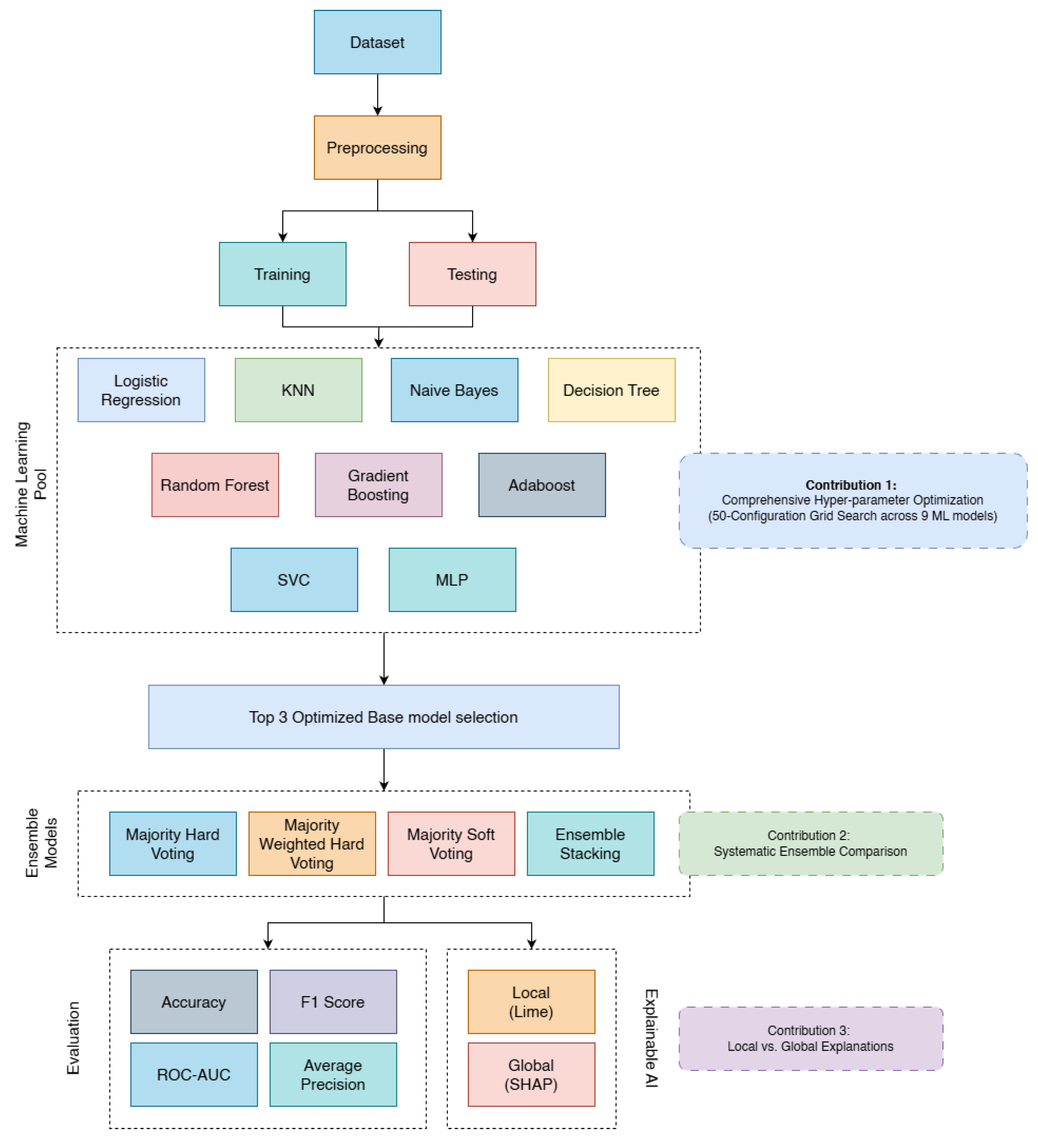
Figure 2.
Pearson Correlation for Dataset-1 and Dataset-2
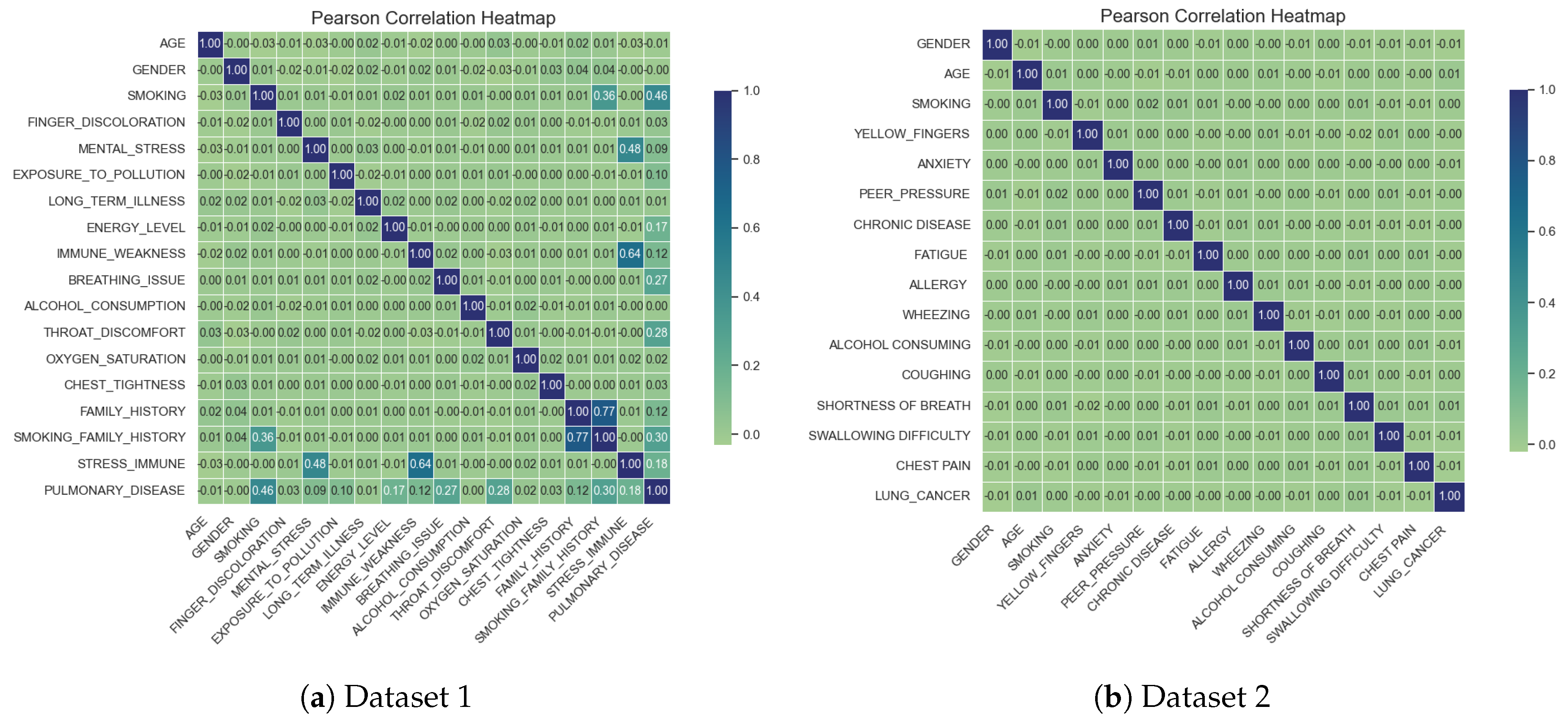
Figure 3.
Class distribution of the Datasets
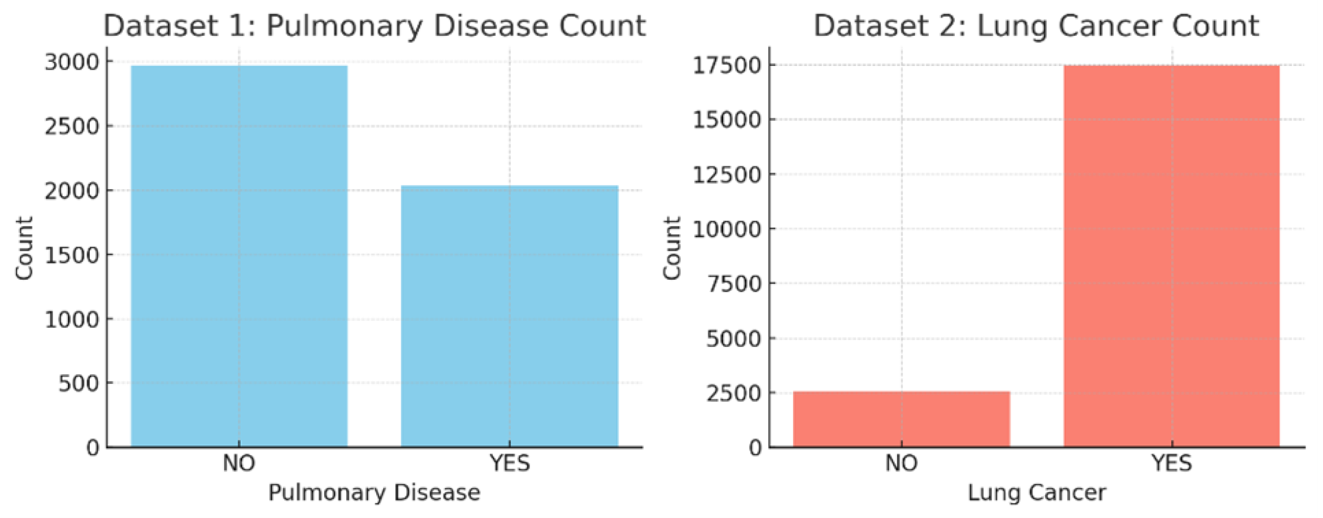
Figure 4.
Precision Recall Curve for Dataset 1
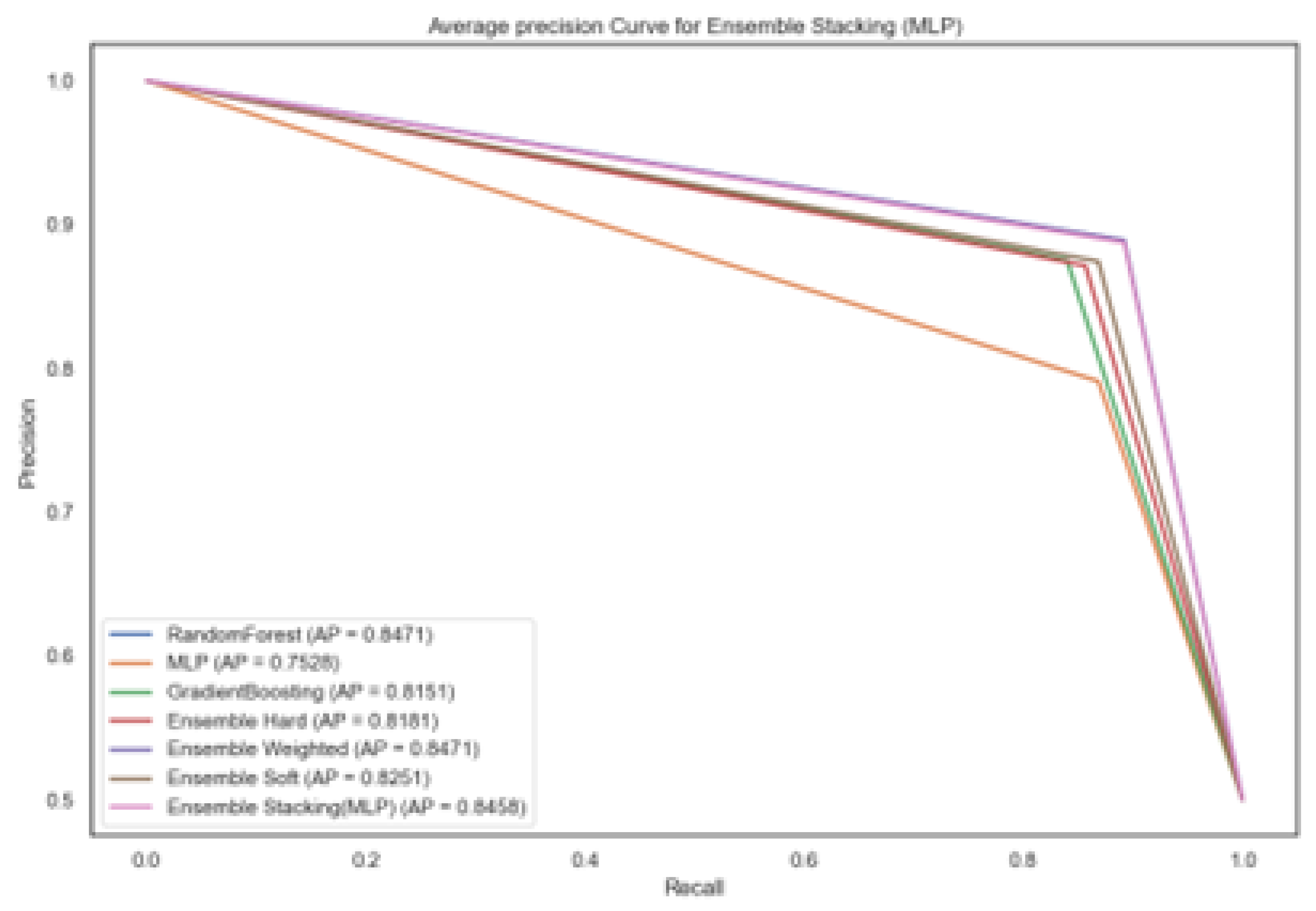
Figure 5.
Confusion Matrix for models trained on Dataset 1
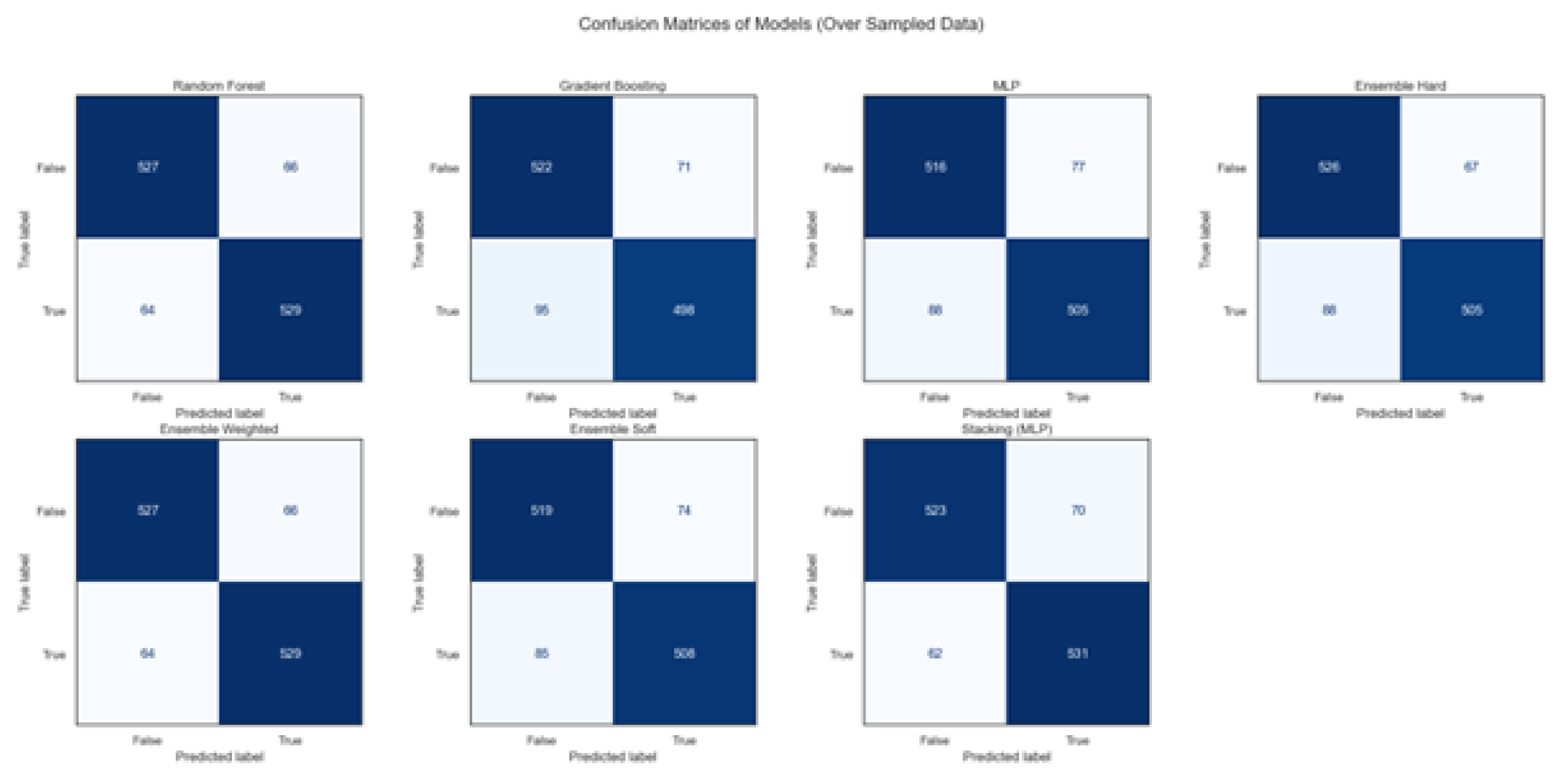
Figure 6.
Precision Recall Curve for Dataset 2
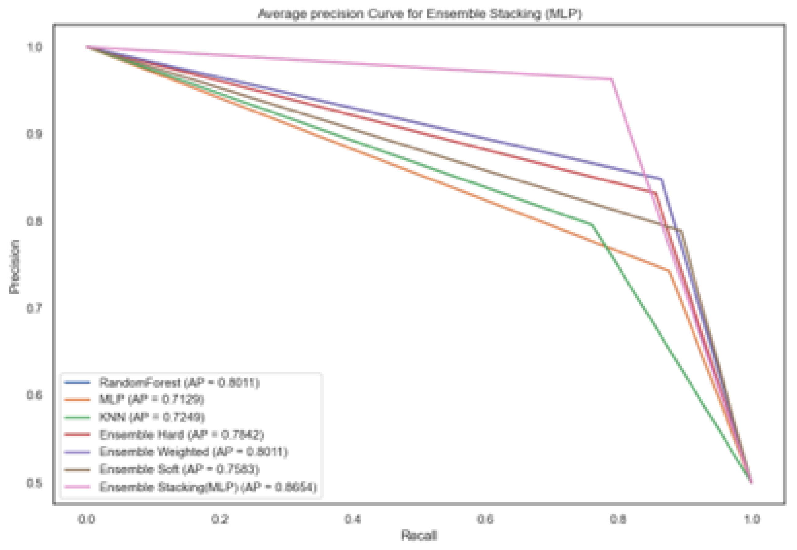
Figure 7.
Confusion Matrix for models trained on Dataset 2
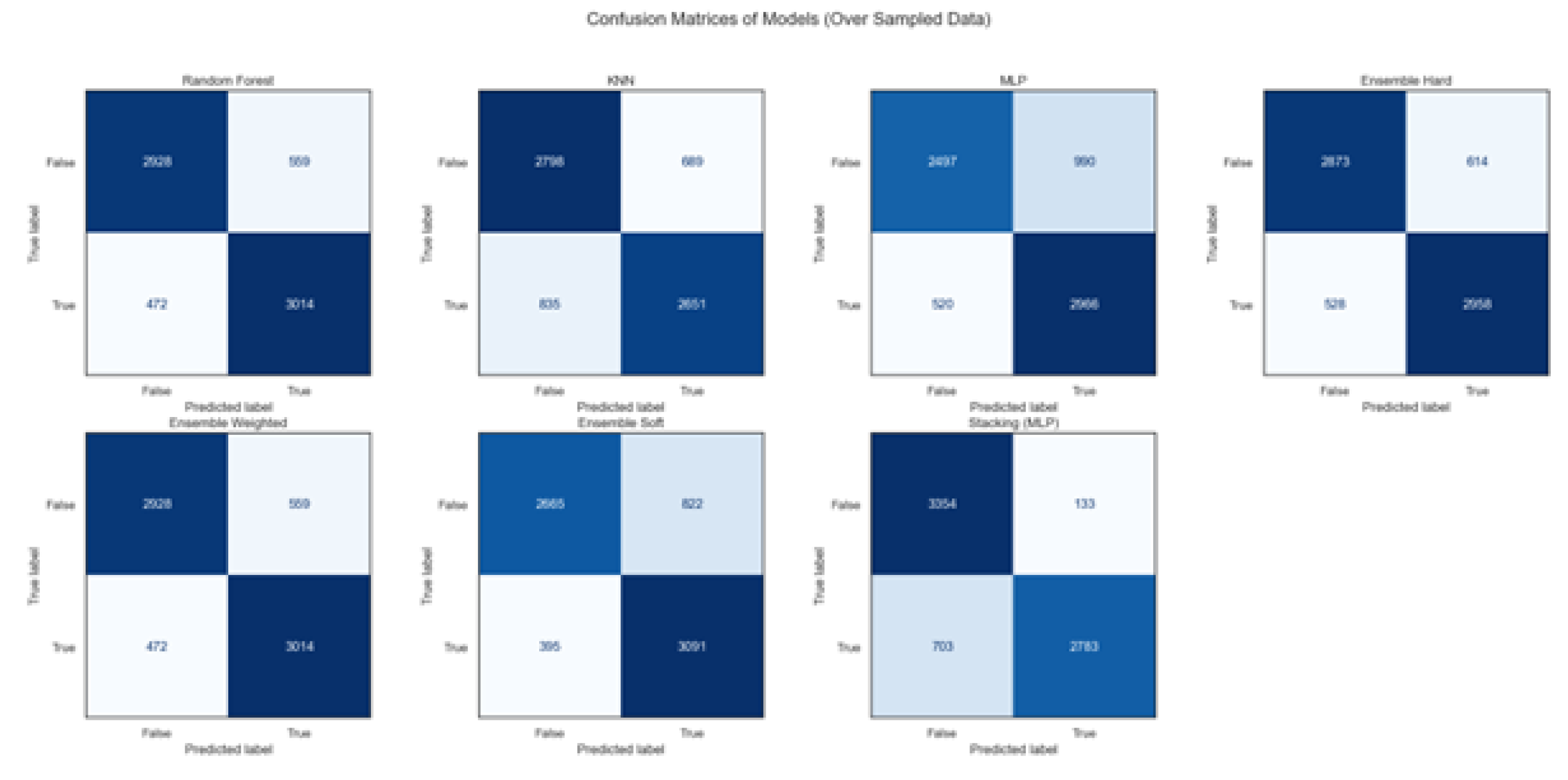
Figure 8.
Lime Explanation for Pulmonary Disease Class in Dataset 1
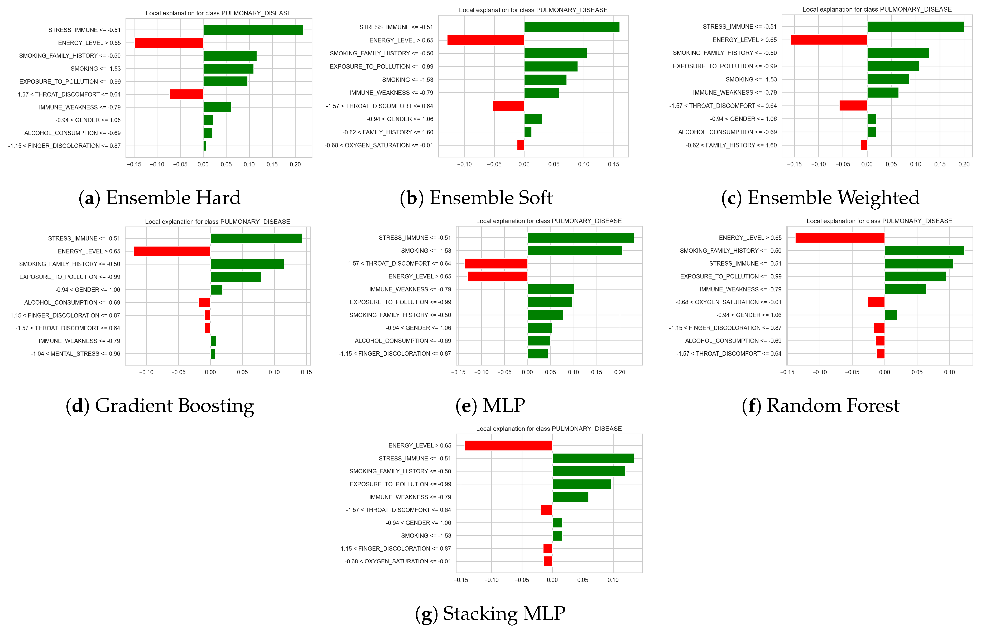
Figure 9.
Lime Explanation for Healthy Class in Dataset 1
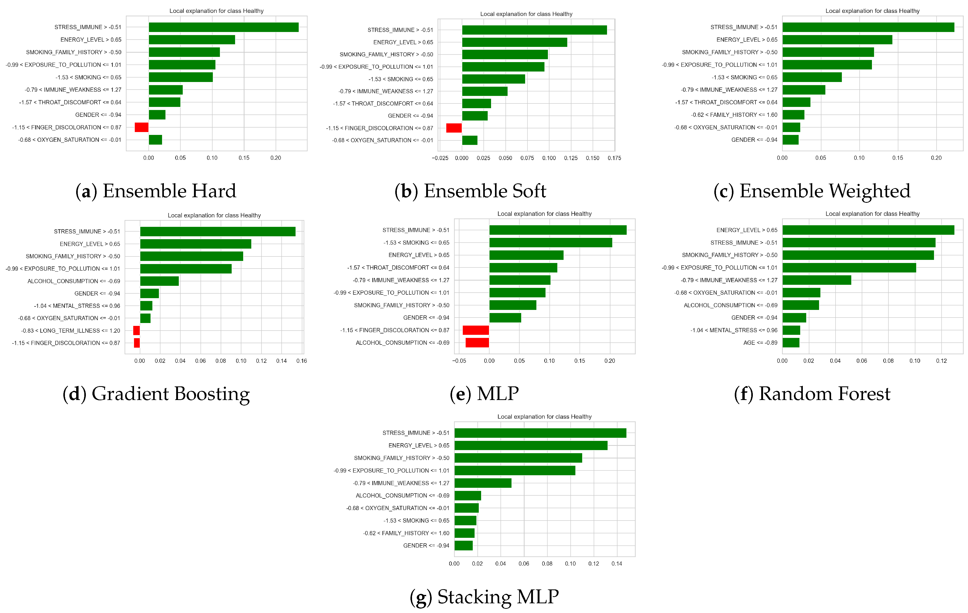
Figure 10.
Lime Explanation for Healthy Class in Dataset 1
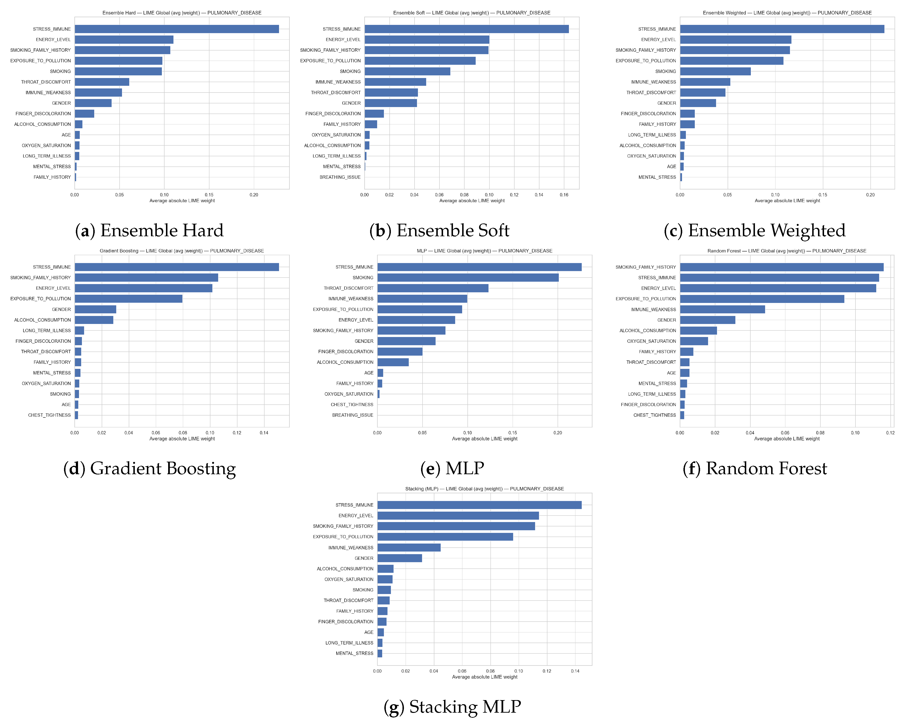
Figure 11.
Lime Explanation for Healthy Class in Dataset 1
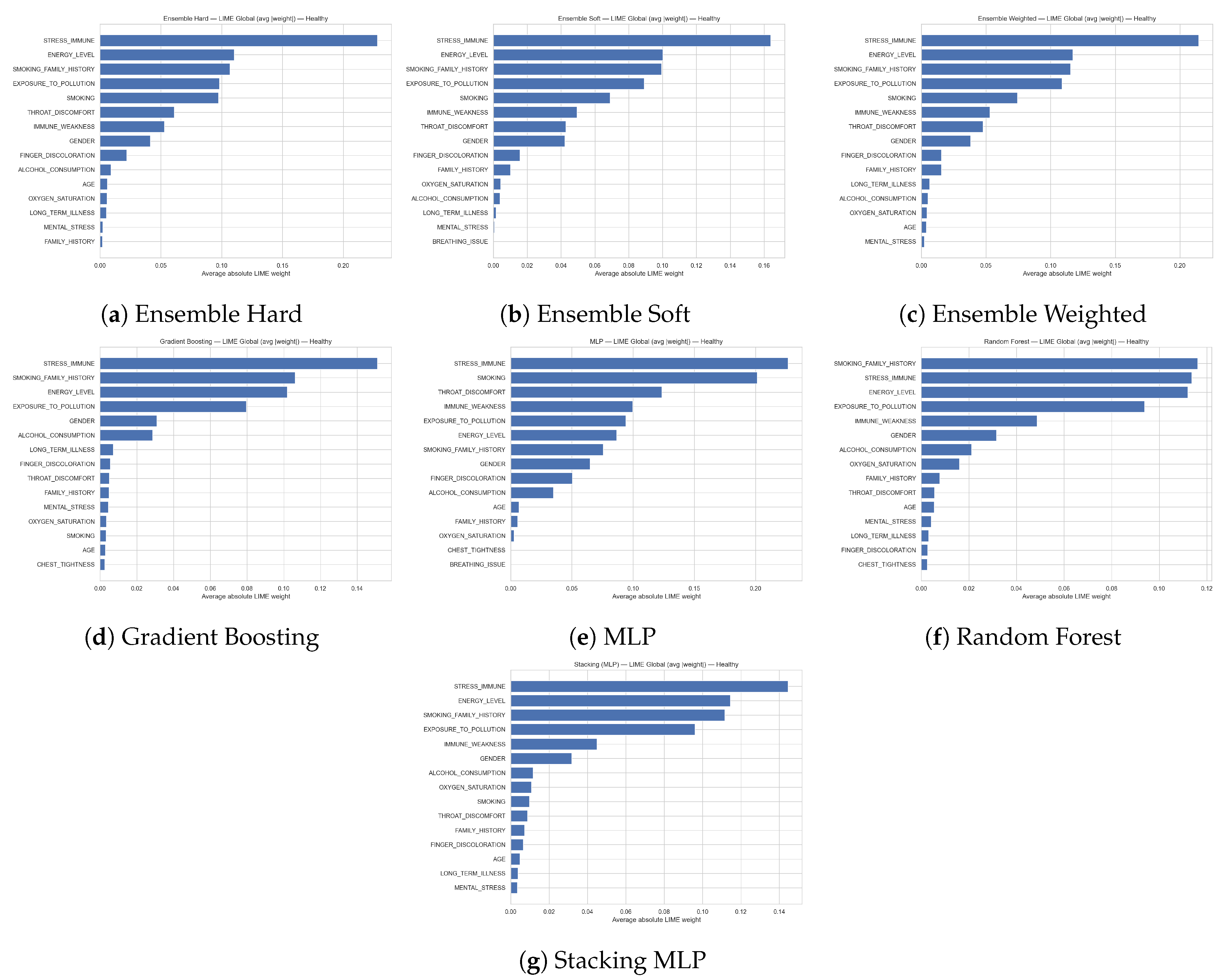
Figure 12.
Lime Explanation for Overall Classes in Dataset 1
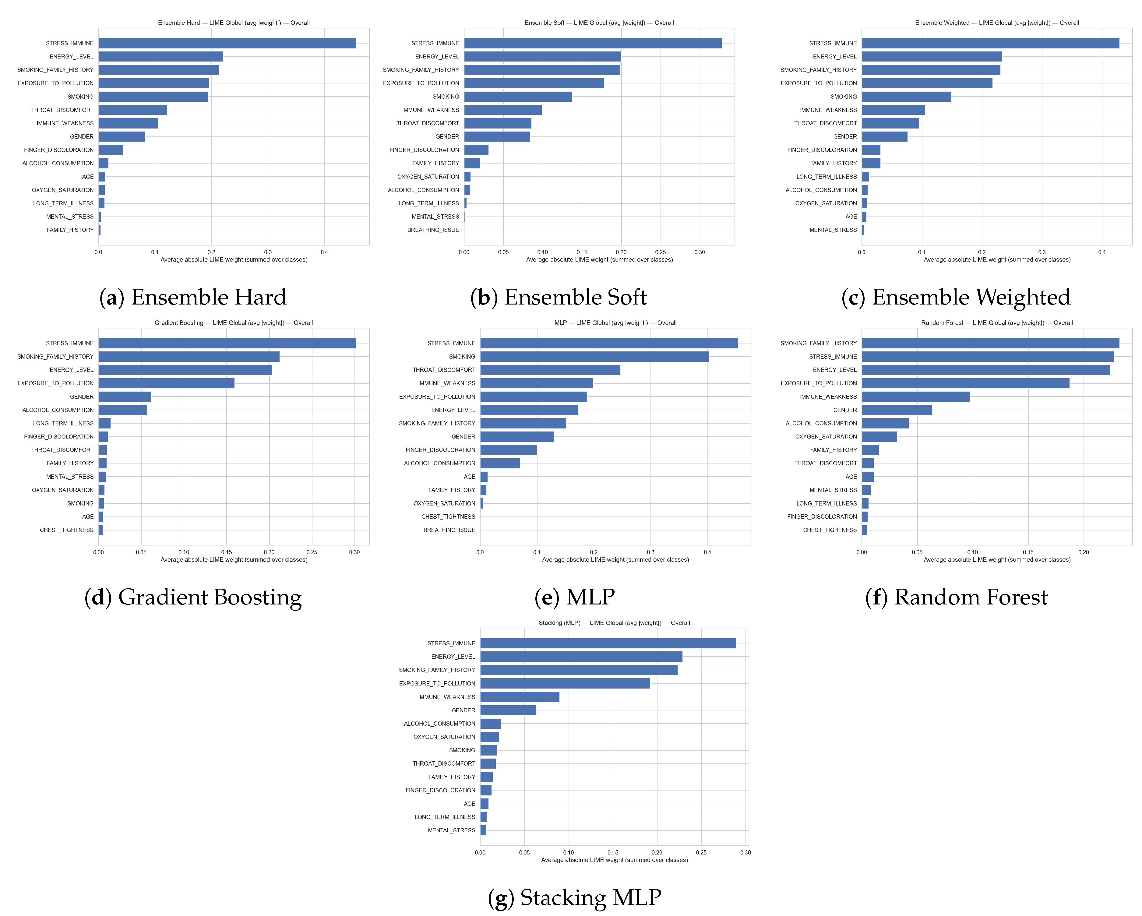
Figure 13.
Lime Explanation for Pulmonary Disease Class in Dataset 2
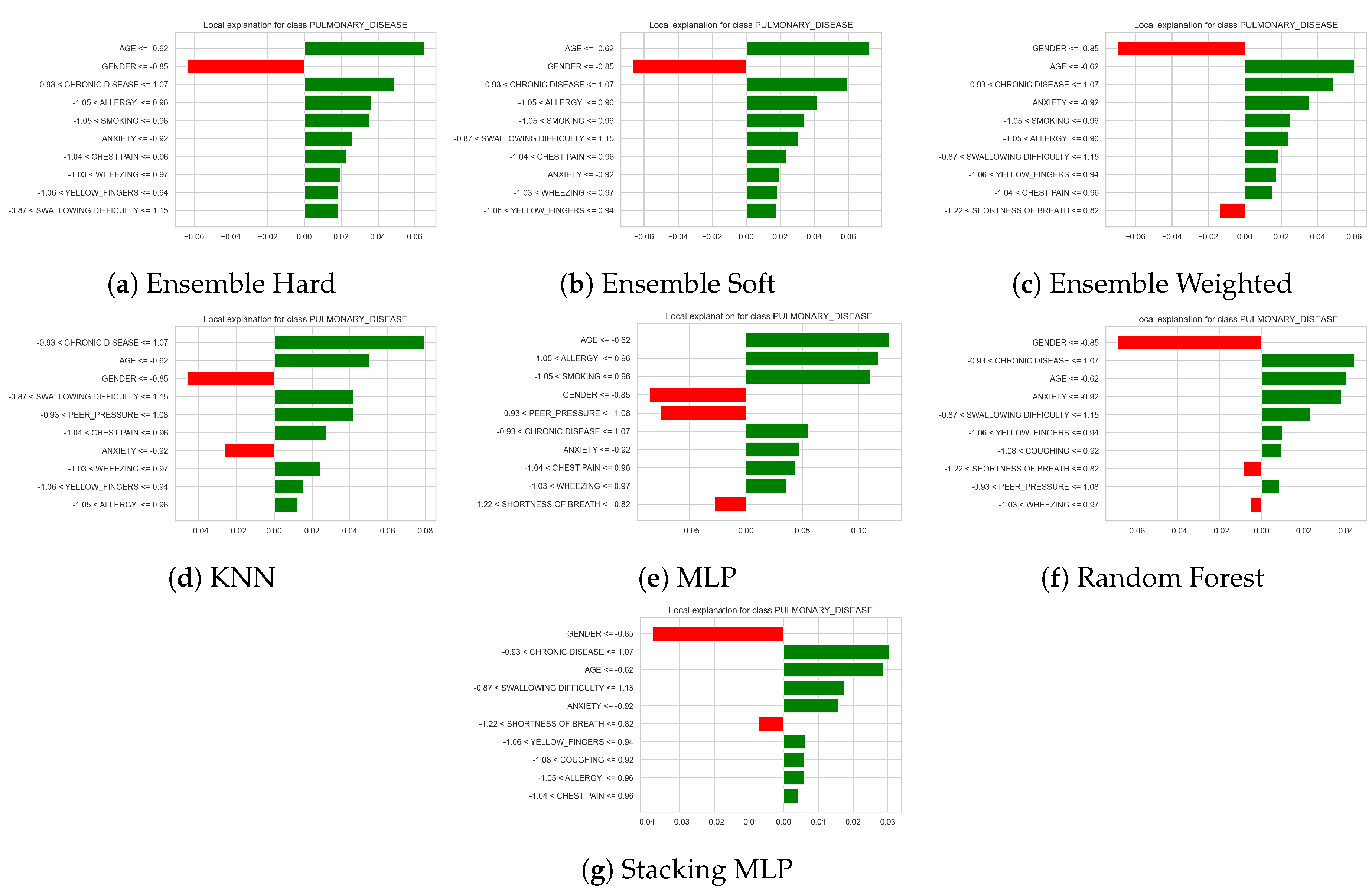
Figure 14.
Lime Explanation for Healthy Class in Dataset 1
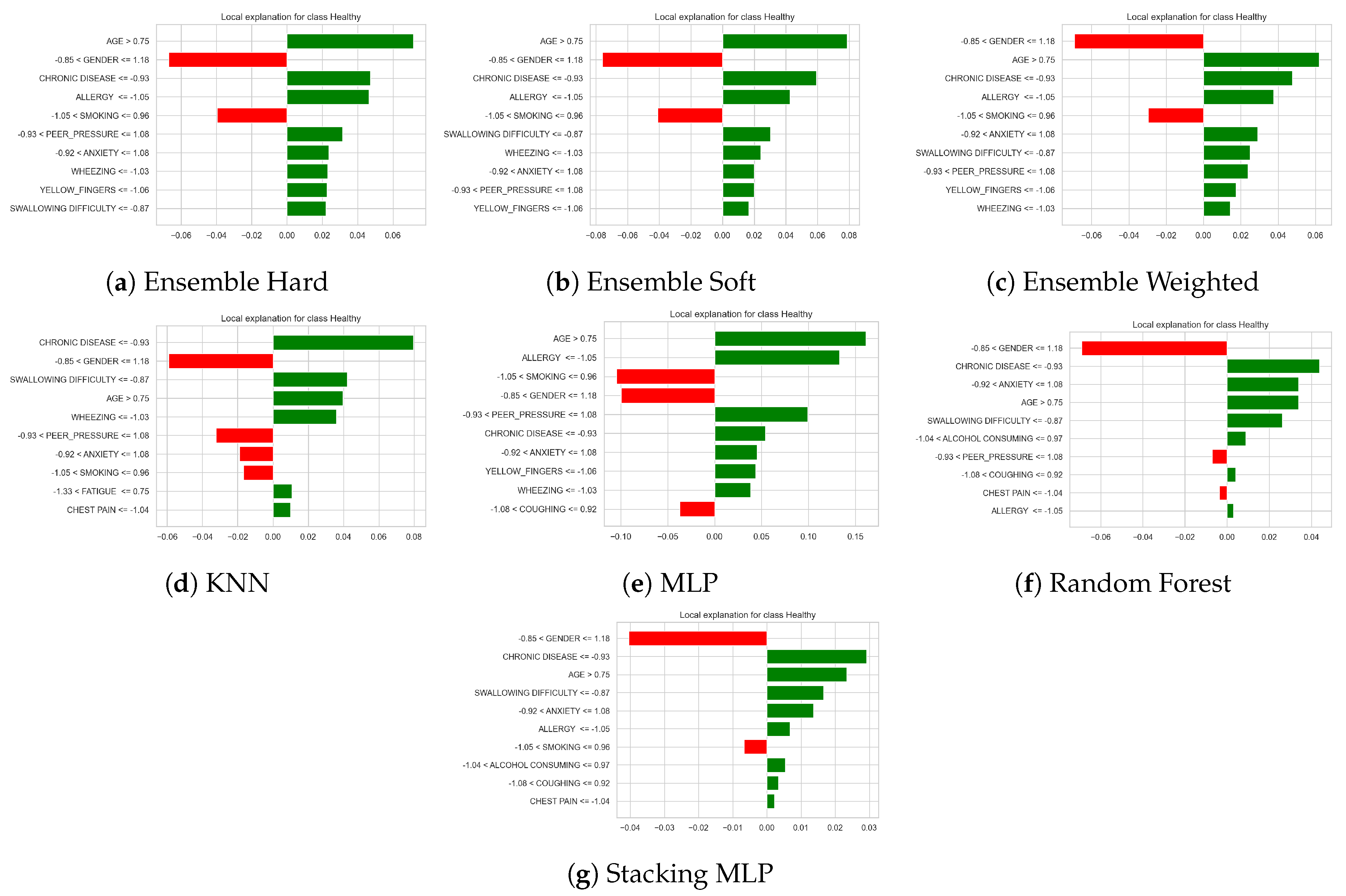
Figure 15.
Lime Explanation for Healthy Class in Dataset 2
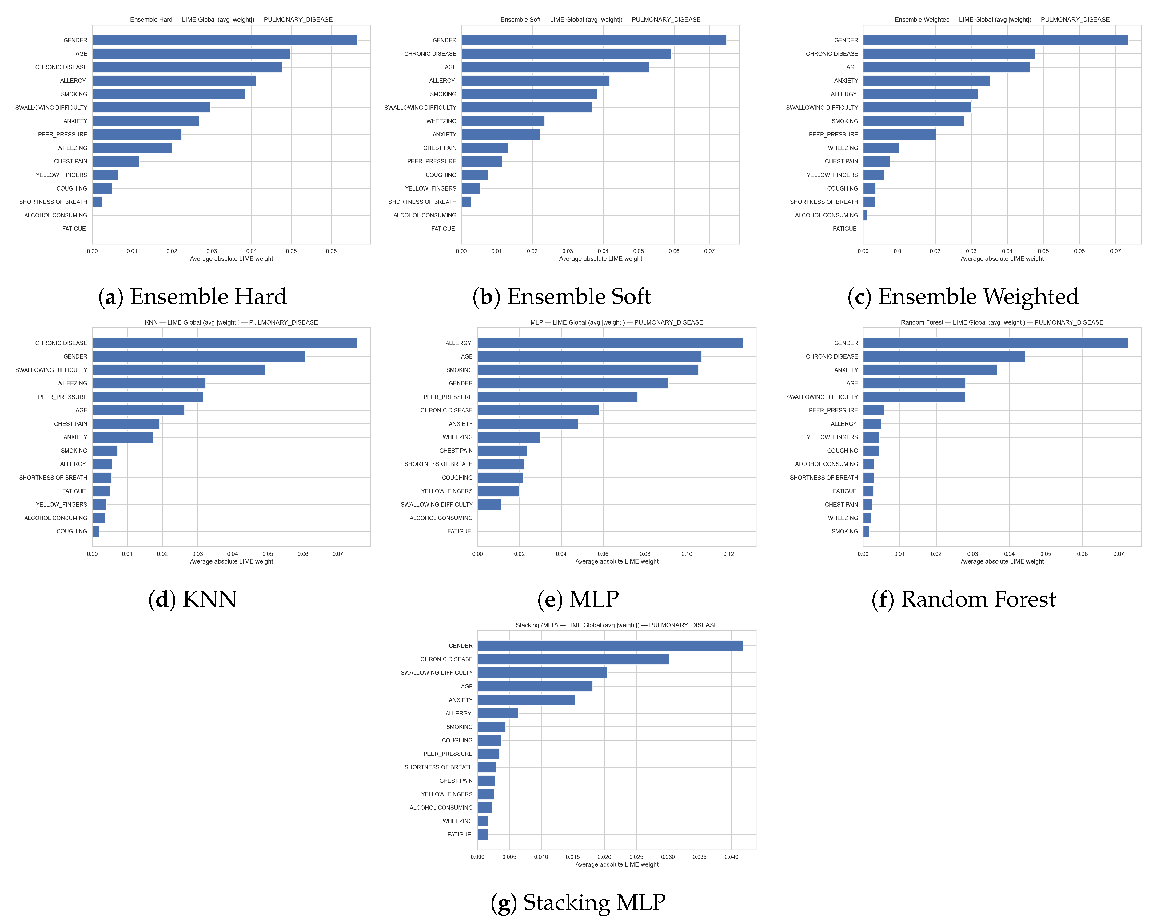
Figure 16.
Lime Explanation for Healthy Class in Dataset 1

Figure 17.
Lime Explanation for Overall Classes in Dataset 2
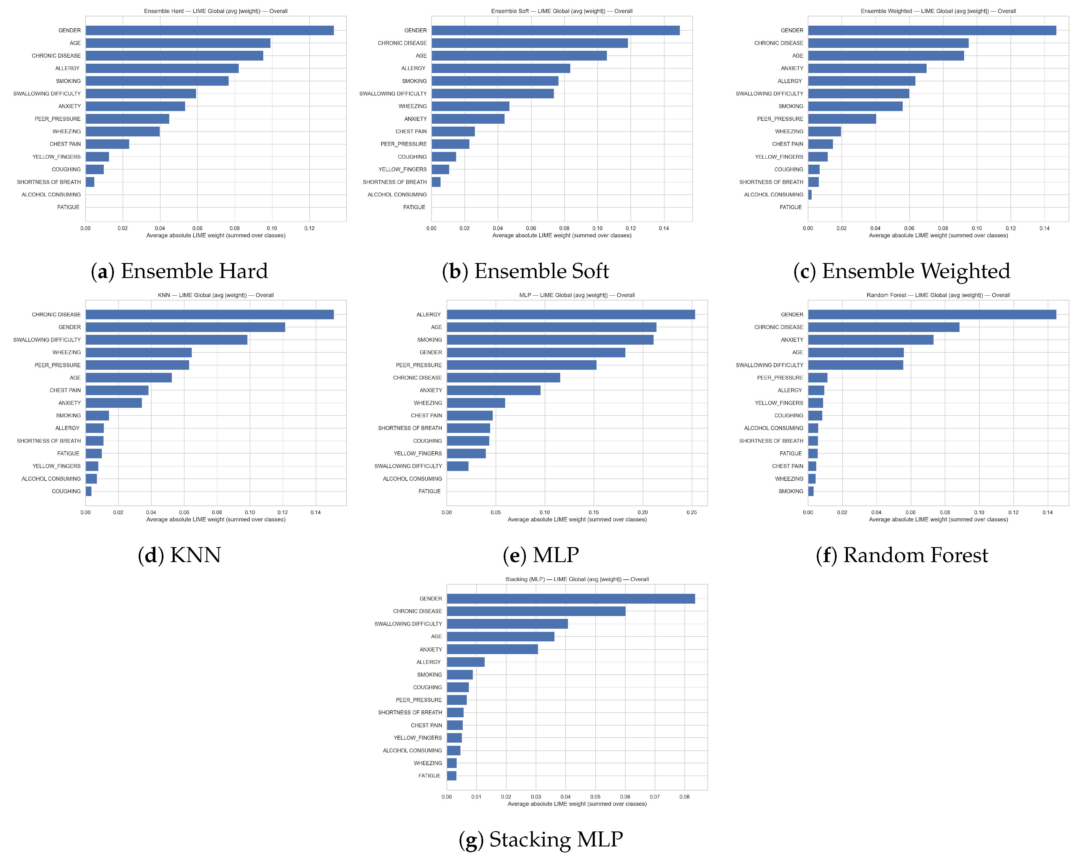
Figure 18.
SHAP Explanation for all Classes in Dataset 1
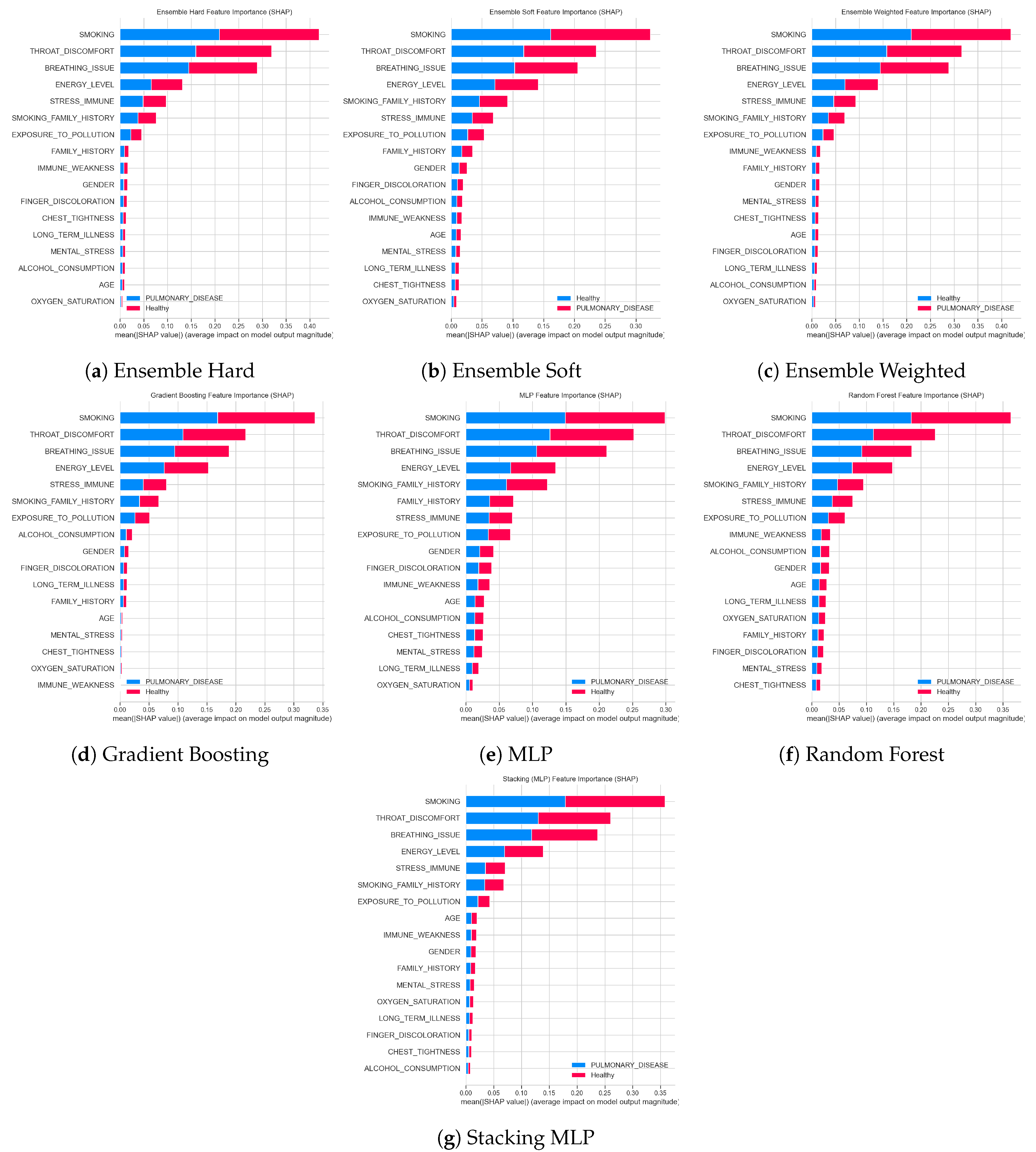
Figure 19.
SHAP Explanation for all Classes in Dataset 2
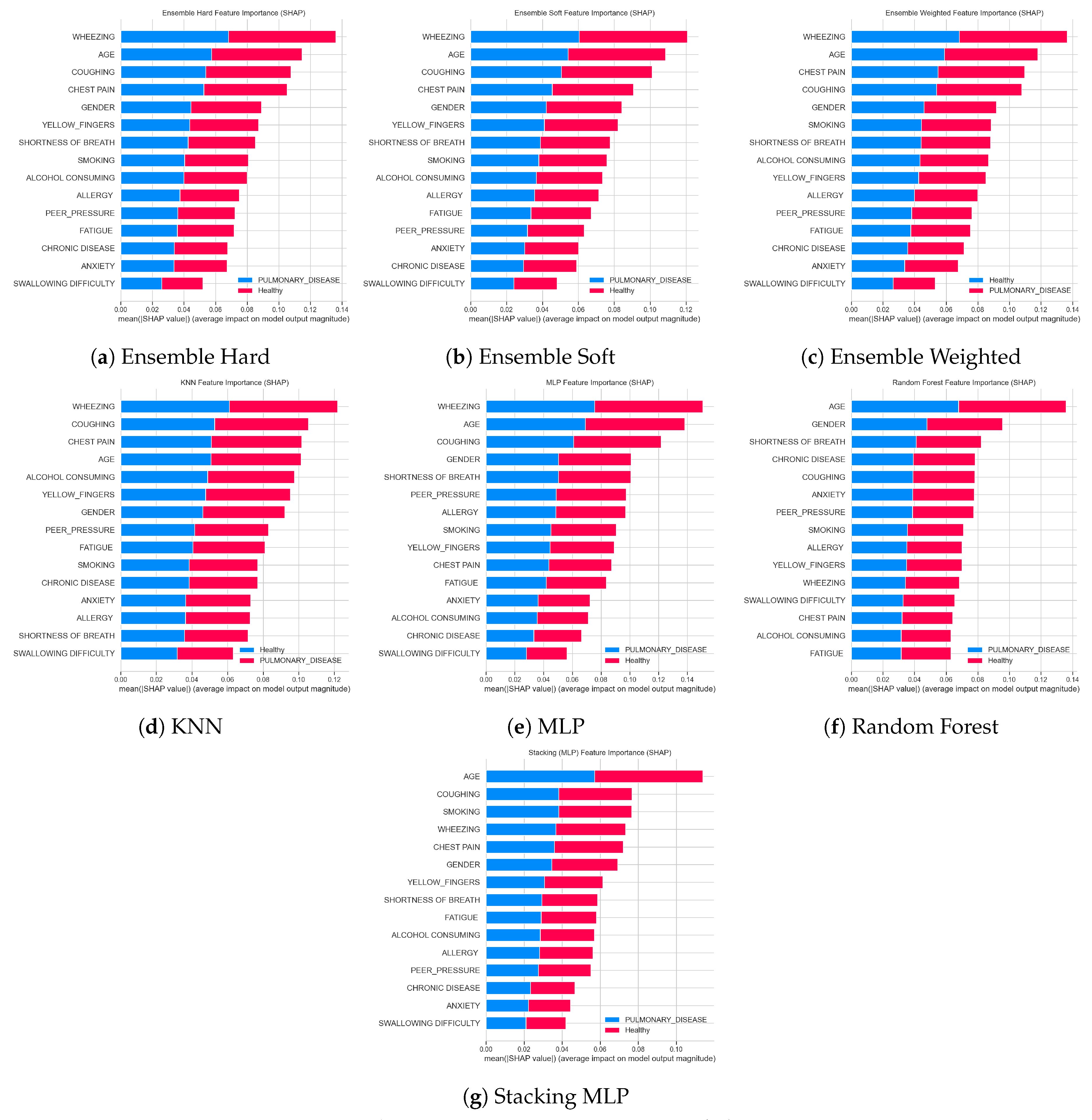
Table 2.
Machine Learning Pool Description.
| Model ID | Model Type | Parameters |
| LR1 | Logistic Regression | penalty=l2, C=0.75, solver=liblinear, multi_class=ovr |
| LR2 | Logistic Regression | penalty=None |
| LR3 | Logistic Regression | penalty=l2, C=0.75, solver=lbfgs |
| LR4 | Logistic Regression | penalty=l2, C=0.5 |
| LR5 | Logistic Regression | penalty=l2, C=1.0 |
| LR6 | Logistic Regression | penalty=l2, C=0.8 |
| KNN | KNN | n_neighbors=2, algorithm=kd_tree, metric=manhattan |
| 3NN | KNN | n_neighbors=3 |
| 5NN | KNN | n_neighbors=5 |
| 6NN | KNN | n_neighbors=6, algorithm=brute, p=1, metric=cosine |
| 9NN | KNN | n_neighbors=9, algorithm=ball_tree, metric=euclidean |
| 10NN | KNN | n_neighbors=10, algorithm=brute, p=2, metric=minkowski |
| NB1 | Naive Bayes | GaussianNB |
| NB2 | Naive Bayes | BernoulliNB |
| DT1 | Decision Tree | criterion=gini, min_samples_leaf=4 |
| DT2 | Decision Tree | criterion=gini, max_features=sqrt, min_samples_leaf=2, min_impurity_decrease=0.01 |
| DT3 | Decision Tree | criterion=gini, max_features=log2, min_samples_leaf=2, min_impurity_decrease=0.01 |
| DT4 | Decision Tree | criterion=entropy, splitter=random, max_depth=6, min_samples_leaf=2 |
| DT5 | Decision Tree | criterion=log_loss, max_depth=8, min_samples_leaf=3, min_impurity_decrease=0.001 |
| RF1 | Random Forest | criterion=entropy, n_estimators=100 |
| RF2 | Random Forest | n_estimators=500 |
| RF3 | Random Forest | n_estimators=1000 |
| RF4 | Random Forest | criterion=log_loss, n_estimators=500 |
| RF5 | Random Forest | criterion=gini, max_features=log2, n_estimators=500 |
| RF6 | Random Forest | criterion=gini, max_features=sqrt, n_estimators=1000, bootstrap=False |
| RF7 | Random Forest | criterion=gini, max_features=log2, n_estimators=500, bootstrap=False |
| RF8 | Random Forest | criterion=entropy, n_estimators=500, bootstrap=False |
| GB1 | Gradient Boosting | n_estimators=500 |
| GB2 | Gradient Boosting | loss=log_loss, n_estimators=1000, criterion=squared_error |
| GB3 | Gradient Boosting | loss=log_loss, n_estimators=400, criterion=friedman_mse |
| GB4 | Gradient Boosting | n_estimators=1100, criterion=squared_error, min_impurity_decrease=0.01 |
| GB5 | Gradient Boosting | loss=log_loss, n_estimators=500, criterion=friedman_mse, min_impurity_decrease=0.001 |
| GB6 | Gradient Boosting | loss=log_loss, n_estimators=800, min_samples_leaf=3, criterion=squared_error |
| GB7 | Gradient Boosting | loss=log_loss, n_estimators=1200, min_impurity_decrease=0.01 |
| GB8 | Gradient Boosting | n_estimators=500, min_samples_split=5, min_impurity_decrease=0.0001 |
| AdaBoost1 | AdaBoost | default |
| AdaBoost2 | AdaBoost | n_estimators=200, algorithm=SAMME |
| AdaBoost3 | AdaBoost | n_estimators=500, algorithm=SAMME, learning_rate=2 |
| AdaBoost4 | AdaBoost | n_estimators=1000, algorithm=SAMME |
| AdaBoost5 | AdaBoost | n_estimators=1200 |
| SVC1 | SVC | probability=True |
| SVC2 | SVC | probability=True, C=0.5, kernel=linear |
| SVC3 | SVC | probability=True, C=0.75, kernel=linear |
| SVC4 | SVC | probability=True, C=1.0, kernel=linear |
| SVC5 | SVC | probability=True, C=1.25, kernel=linear |
| MLP1 | MLP | max_iter=500 |
| MLP2 | MLP | max_iter=200 |
| MLP3 | MLP | learning_rate=adaptive, max_iter=500 |
| MLP4 | MLP | learning_rate=invscaling, max_iter=1000 |
| MLP5 | MLP | hidden_layer_sizes=(100,100), max_iter=1000 |
Table 3.
Evaluation of Machine Learning Pool.
| Model ID | Dataset 1 | Dataset 2 | ||
|---|---|---|---|---|
| Accuracy | F1 | Accuracy | F1 | |
| LR1 | 0.845148 | 0.849126 | 0.61285 | 0.616319 |
| LR2 | 0.84557 | 0.849425 | 0.612814 | 0.61627 |
| LR3 | 0.845148 | 0.849126 | 0.612814 | 0.61627 |
| LR4 | 0.845148 | 0.849126 | 0.612814 | 0.61627 |
| LR5 | 0.845148 | 0.849054 | 0.612814 | 0.61627 |
| LR6 | 0.844937 | 0.848887 | 0.612814 | 0.61627 |
| KNN | 0.784177 | 0.764544 | 0.77093 | 0.765034 |
| 3NN | 0.816667 | 0.822323 | 0.751425 | 0.775123 |
| 5NN | 0.821941 | 0.828337 | 0.74239 | 0.769882 |
| 6NN | 0.83903 | 0.835358 | 0.739271 | 0.748684 |
| 9NN | 0.829114 | 0.835404 | 0.726399 | 0.755462 |
| 10NN | 0.845992 | 0.844402 | 0.725145 | 0.740095 |
| NB1 | 0.822785 | 0.825935 | 0.613818 | 0.618514 |
| NB2 | 0.822152 | 0.828467 | 0.612276 | 0.616453 |
| DT1 | 0.81962 | 0.816134 | 0.736259 | 0.74012 |
| DT2 | 0.718565 | 0.765519 | 0.499839 | 0.33327 |
| DT3 | 0.718565 | 0.765519 | 0.499839 | 0.33327 |
| DT4 | 0.823207 | 0.81399 | 0.499839 | 0.33327 |
| DT5 | 0.855907 | 0.851557 | 0.581765 | 0.589635 |
| RF1 | 0.8827 | 0.880105 | 0.832813 | 0.837466 |
| RF2 | 0.879536 | 0.876935 | 0.834283 | 0.838806 |
| RF3 | 0.879958 | 0.877382 | 0.833566 | 0.838062 |
| RF4 | 0.882068 | 0.879572 | 0.833244 | 0.838032 |
| RF5 | 0.879536 | 0.876935 | 0.834283 | 0.838806 |
| RF6 | 0.88481 | 0.88294 | 0.836506 | 0.838439 |
| RF7 | 0.886076 | 0.884351 | 0.836435 | 0.838386 |
| RF8 | 0.822785 | 0.823382 | 0.806747 | 0.819663 |
| GB1 | 0.858017 | 0.857035 | 0.649564 | 0.658597 |
| GB2 | 0.852321 | 0.851531 | 0.659711 | 0.669583 |
| GB3 | 0.859705 | 0.858773 | 0.647987 | 0.656373 |
| GB4 | 0.778059 | 0.793244 | 0.500018 | 0.666683 |
| GB5 | 0.855696 | 0.854825 | 0.650389 | 0.659524 |
| GB6 | 0.844093 | 0.842322 | 0.597218 | 0.609395 |
| GB7 | 0.778059 | 0.793244 | 0.500018 | 0.666683 |
| GB8 | 0.863502 | 0.861716 | 0.630168 | 0.637603 |
| AdaBoost1 | 0.827426 | 0.836456 | 0.61493 | 0.616302 |
| AdaBoost2 | 0.827426 | 0.836237 | 0.616077 | 0.619523 |
| AdaBoost3 | 0.697046 | 0.689755 | 0.542397 | 0.537384 |
| AdaBoost4 | 0.834388 | 0.84217 | 0.615969 | 0.618537 |
| AdaBoost5 | 0.832278 | 0.840148 | 0.613854 | 0.616122 |
| SVC1 | 0.861814 | 0.860198 | 0.68108 | 0.694091 |
| SVC2 | 0.844304 | 0.845031 | 0.613424 | 0.622187 |
| SVC3 | 0.844304 | 0.84497 | 0.613352 | 0.622116 |
| SVC4 | 0.844726 | 0.845385 | 0.613316 | 0.622015 |
| SVC5 | 0.844937 | 0.845565 | 0.613245 | 0.621969 |
| MLP1 | 0.85 | 0.84861 | 0.676849 | 0.679861 |
| MLP2 | 0.864557 | 0.862641 | 0.676455 | 0.683033 |
| MLP3 | 0.85 | 0.84861 | 0.676849 | 0.679861 |
| MLP4 | 0.839241 | 0.837976 | 0.676849 | 0.679861 |
| MLP5 | 0.83038 | 0.832261 | 0.780252 | 0.791777 |
Table 4.
Model Comparison on Dataset 1.
| Model | Accuracy | F1 Score | ROC AUC | Average Precision |
|---|---|---|---|---|
| Gradient Boosting | 0.860 | 0.860 | 0.860 | 0.815 |
| MLP | 0.861 | 0.861 | 0.861 | 0.813 |
| Random Forest | 0.890 | 0.890 | 0.890 | 0.847 |
| Ensemble Hard | 0.869 | 0.869 | 0.869 | 0.826 |
| Ensemble Weighted | 0.890 | 0.890 | 0.890 | 0.847 |
| Ensemble Soft | 0.866 | 0.866 | 0.866 | 0.819 |
| Stacking (MLP) | 0.889 | 0.889 | 0.889 | 0.846 |
Table 5.
Model Comparison on Dataset 2.
| Model | Accuracy | F1 Score | ROC AUC | Average Precision |
|---|---|---|---|---|
| Random Forest | 0.855 | 0.854 | 0.855 | 0.801 |
| MLP | 0.786 | 0.784 | 0.786 | 0.712 |
| KNN | 0.783 | 0.783 | 0.783 | 0.725 |
| Ensemble Hard | 0.841 | 0.841 | 0.841 | 0.784 |
| Ensemble Weighted | 0.855 | 0.854 | 0.855 | 0.801 |
| Ensemble Soft | 0.827 | 0.827 | 0.827 | 0.758 |
| Ensemble Stacking (MLP) | 0.879 | 0.878 | 0.879 | 0.865 |
Disclaimer/Publisher’s Note: The statements, opinions and data contained in all publications are solely those of the individual author(s) and contributor(s) and not of MDPI and/or the editor(s). MDPI and/or the editor(s) disclaim responsibility for any injury to people or property resulting from any ideas, methods, instructions or products referred to in the content. |
© 2025 by the authors. Licensee MDPI, Basel, Switzerland. This article is an open access article distributed under the terms and conditions of the Creative Commons Attribution (CC BY) license (http://creativecommons.org/licenses/by/4.0/).
Copyright: This open access article is published under a Creative Commons CC BY 4.0 license, which permit the free download, distribution, and reuse, provided that the author and preprint are cited in any reuse.


