1. Introduction
Injection molding is a key plastic manufacturing process widely used in industries such as automotive, aerospace, electronics, healthcare, and consumer goods. It is valued for producing complex parts with high precision, good dimensional accuracy, and low cost in large-scale production, ensuring consistent quality and reliability (Goodship, 2017; Menges et al., 2001; Osswald & Hernández-Ortiz, 2006; Rosato & et al., 2007). However, the core complexity bottleneck in injection molding lies in optimizing the intertwined decision variables, including melt temperature, injection pressure, filling speed, packing conditions, and cooling strategies. These variables have cascading effects on conflicting objectives, including cycle time, dimensional accuracy, structural performance, material efficiency, and surface quality. Traditional optimization methods struggle to manage these nonlinear, high-dimensional relationships, particularly due to their high computational demands, making surrogate-assisted optimization fundamental (Gaspar-Cunha et al., 2025a).
This complexity is particularly evident in the design of injection molds with advanced cooling systems, such as conformal cooling channels (CCCs). By closely following the cavity geometry, CCCs improve cooling uniformity, reduce cycle time, limit warpage and shrinkage, and enhance part quality (S. Feng et al., 2021; Silva et al., 2022). However, empirical and heuristic approaches often struggle with the geometric constraints and multiple conflicting objectives involved in CCC optimization, highlighting the need for more advanced and robust optimization frameworks (Gaspar-Cunha et al., 2025a).
Recent advances in additive manufacturing, particularly Direct Metal Laser Sintering (DMLS), have enabled the fabrication of complex CCC geometries and the integration of additional features, such as embedded sensors and improved heat-transfer structures (Chung & Das, 2018; Wei et al., 2020; Wu & Tovar, 2018). While these advances expand design possibilities, they also increase problem complexity by introducing new decision variables, further reinforcing the need for adaptive and intelligent optimization methods.
To address these issues, this study uses Principal Component Analysis (PCA), Non-Linear PCA (NL-PCA), Mutual Information and clustering (MI/C), Artificial Neural Networks (ANNs), and Multi-Objective Evolutionary Algorithms (MOEAs). PCA and similar methods help select the most important objectives, while ANNs serve as fast, accurate substitutes for costly simulations, reducing computation time (Gaspar-Cunha & Vieira, 2005; Gaspar-Cunha et al., 2022; Gaspar-Cunha et al., 2025a; Jolliffe & Cadima, 2016).
Multi-objective evolutionary algorithms, particularly NSGA-III, are then used to efficiently explore the design space and identify Pareto-optimal trade-offs, providing designers with multiple viable solutions (D. Deb et al., 2014). Unlike previous studies that focused primarily on cycle time, shrinkage, and warpage, this work also considers detailed performance indicators, including thermal profiles, transient thermal behavior, and structural response (Gaspar-Cunha et al., 2025b). Particularly, unlike prior work that optimized only basic parameters, our framework integrates advanced performance metrics, offering a comprehensive approach that enhances both the predictive accuracy and applicability of the optimization results in real-world scenarios.
This work extends a previous publication where the initial methodology is presented (Gaspar-Cunha et a., 2025b) to: i) improve the methodology used to select the objectives, and ii) study the effect of the sampling density. Therefore, the main goal of this research is to evaluate the effectiveness of combining PCA, MI/clustering, ANNs, and MOEAs for optimizing CCC designs in real-world injection molding problems. The approach involves selecting objectives, training ANN surrogate models using Moldex-3D simulations, and running multi-objective optimizations for cooling channel designs. The study also examines various algorithmic configurations, including the number of simulation samples, dimensionality-reduction methods, gate locations, and ANN models.
Overall, this work demonstrates the strong potential of integrated AI-based techniques to capture complex nonlinear interactions among multiple conflicting objectives, thereby improving mold design accuracy, production efficiency, product quality, and economic viability.
The paper is structured as follows:
Section 2 reviews the literature,
Section 3 explains the methods,
Section 4 presents the experimental results, and
Section 5 offers conclusions and suggestions for future research.
2. Injection Molding Process
2.1. Brief Description
Injection molding is a key manufacturing process used in many industries to produce plastic parts with high dimensional accuracy, complex geometries, and consistent quality at low cost (Rosato & et al., 2007). It is especially suitable for mass production due to its high productivity, precision, reliability, and repeatability.
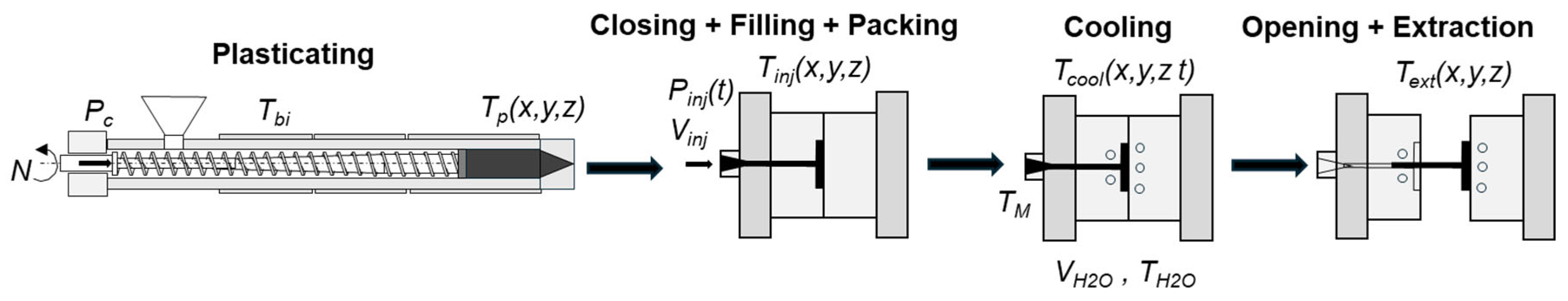
The injection molding cycle includes the main stages shown in
Figure 1 (Faes, 2000; Rosato & et al., 2007):
Plasticating: Solid polymer pellets are fed from the hopper and melted inside a heated barrel by a rotating screw. This stage ensures proper temperature control of the molten polymer before injection.
Mold Closing: The two mold halves align and close securely, forming a cavity that defines the final shape of the part.
Filling: The molten polymer is injected into the closed mold at high pressure and speed, allowing complete filling of complex cavity geometries.
Packing: Pressure is maintained after filling to compensate for material shrinkage during solidification, improving part density and reducing defects.
Cooling: Heat is removed from the polymer through cooling channels in the mold. This stage is critical to ensure dimensional accuracy, structural integrity, and minimal warpage.
Mold Opening and Ejection: After sufficient cooling, the mold opens, and the solidified part is ejected, preparing the mold for the next cycle.
The duration of each stage depends on the material and part design, but cooling typically accounts for 50–80% of the total cycle time, making it the dominant factor in cycle-time reduction efforts (Silva et al., 2022). Improving cooling efficiency is therefore essential to reduce production time without affecting part quality.
At the same time, during cooling, the next polymer shot is plasticized in the barrel, allowing a continuous and efficient production process (Rosato & et al., 2007).
2.2. Optimization Problem
Improving the injection molding (IM) process requires optimizing several interrelated variables to enhance performance, reduce waste, and maintain high product quality. IM optimization, therefore, involves defining decision variables, objectives, and optimization methods and integrating them with numerical simulation tools.
Decision variables are generally grouped into: (i) process conditions, such as injection pressure and velocity, packing pressure and time, melt and mold temperatures, cooling time, and cycle time; and (ii) mold design parameters, including gate, runner, and cavity dimensions, as well as the geometry and layout of cooling channels (e.g., number, diameter, length, and position). This also includes conformal cooling channels (CCCs) enabled by additive manufacturing.
Typical objectives include reducing cooling and total cycle times, shrinkage, warpage, internal stresses, dimensional deviations, part weight, material usage, and defects (e.g., sink marks, weld lines, and flow marks), while improving temperature uniformity, part quality, and dimensional stability.
Multi-objective optimization (MOO) methods are widely used in injection molding to manage these conflicting goals. Examples include Alam & Kamal (2003, 2004, 2005), Fernandes et al. (2010, 2012), and Xu et al. (2012). Advanced approaches that combine MOEAs with surrogate models, such as Response Surface Methodology (RSM) and artificial neural networks (ANNs), enable efficient design space exploration with reduced computational cost (Gaspar-Cunha et al., 2025a).
2.3. Modelling Using Moldex3D
Simulation is crucial in effectively achieving the objectives outlined above. Moldex3D is a powerful simulation tool widely used for modeling and optimizing injection molding processes. It enables comprehensive 3D analysis of each phase of the molding cycle, from filling to cooling and warpage prediction (Osswald & Hernández-Ortiz, 2006).
In the context of process optimization, Moldex3D allows (Kitayama et al., 2018; Nguyen et al., 2023):
Simulation of polymer flow, packing behavior, cooling rates, and temperature gradients.
Evaluation of defect formation, such as weld lines, voids, sink marks, and air traps.
Visualization and analysis of internal mold temperature distribution and flow front progression.
Design and simulation of CCCs, including those fabricated using additive manufacturing techniques such as DMLS.
By integrating Moldex3D simulations with optimization algorithms, such as evolutionary algorithms or hybrid methods, one can develop predictive models (e.g., via ANN or RSM) and systematically explore decision variable combinations to find optimal trade-offs among multiple objectives (Fernandes et al., 2012; Gaspar-Cunha & Viana, 2005).
2.4. Designing CCCs
Conformal cooling channels (CCCs) significantly improve thermal control in injection molding, affecting cycle time, energy consumption, and part quality (Gaspar-Cunha et al., 2025a). Early studies showed that CCCs outperform conventional cooling by reducing warpage, improving temperature uniformity, and shortening cycle times (Brooks & Brigden, 2016; Mazur et al., 2017; Tuteski & Kočov, 2018; van As et al., 2017). Additive manufacturing has enabled the fabrication of more complex CCC geometries with improved performance.
Recent research increasingly uses computational tools. Konuskan et al. (2023) applied LSTM neural networks to optimize cooling, while Zacharski et al. (2023) demonstrated the flexibility and lower cost of modular CCC molds. Optimization methods, from empirical approaches to evolutionary algorithms (EA), have been used to improve channel design and process conditions (Q. Q. Feng & Zhou, 2019; Ferreira et al., 2010; Hashimoto et al., 2020; S. Jahan et al., 2019; Kim & Lee, 2019; Zhai et al., 2009), but many studies still focus on single objectives.
Multi-objective (MO) optimization is required to balance cooling performance, cost, and structural integrity, as shown by Kanbur et al. (2022) and Le Goff & Garcia (2011). Topology optimization (TO), often combined with generative design and machine learning, has been used to create advanced CCCs (Jahan et al., 2016, 2017; Wu & Tovar, 2018; Wilson et al., 2024).
AI and surrogate models, such as Kriging and neural networks, reduce computational cost and improve prediction accuracy (Zhao & Cheng, 2016; Kanbur et al., 2020; X. Liu et al., 2022), although empirical methods are still common (Hsu et al., 2013; Saifullah et al., 2012).
Future research should emphasize MO algorithms (e.g., NSGA-II, MOEA/D), stronger integration of simulation tools like Moldex3D with experiments (S. Jahan et al., 2019; Shen et al., 2019), sustainability metrics such as LCA, AI-based real-time optimization (Gao et al., 2023), and industrial validation (Eiamsa-Ard & Wannissorn, 2015). Thermal–mechanical coupling is also critical, as shown by S. Jahan et al. (2019), highlighting the need for accurate multi-physics models.
3. Optimization of Injection Molding
3.1. Methodology
The proposed methodology combines high-fidelity simulation, data-driven models, and evolutionary optimization to design conformal cooling channels for injection molds. Moldex3D is used to simulate each mold design and generate multiple performance metrics. Because optimizing multiple objectives directly is computationally expensive and involves strong trade-offs, dimensionality reduction and surrogate modeling are used to simplify the problem (Gaspar-Cunha et al., 2025a).
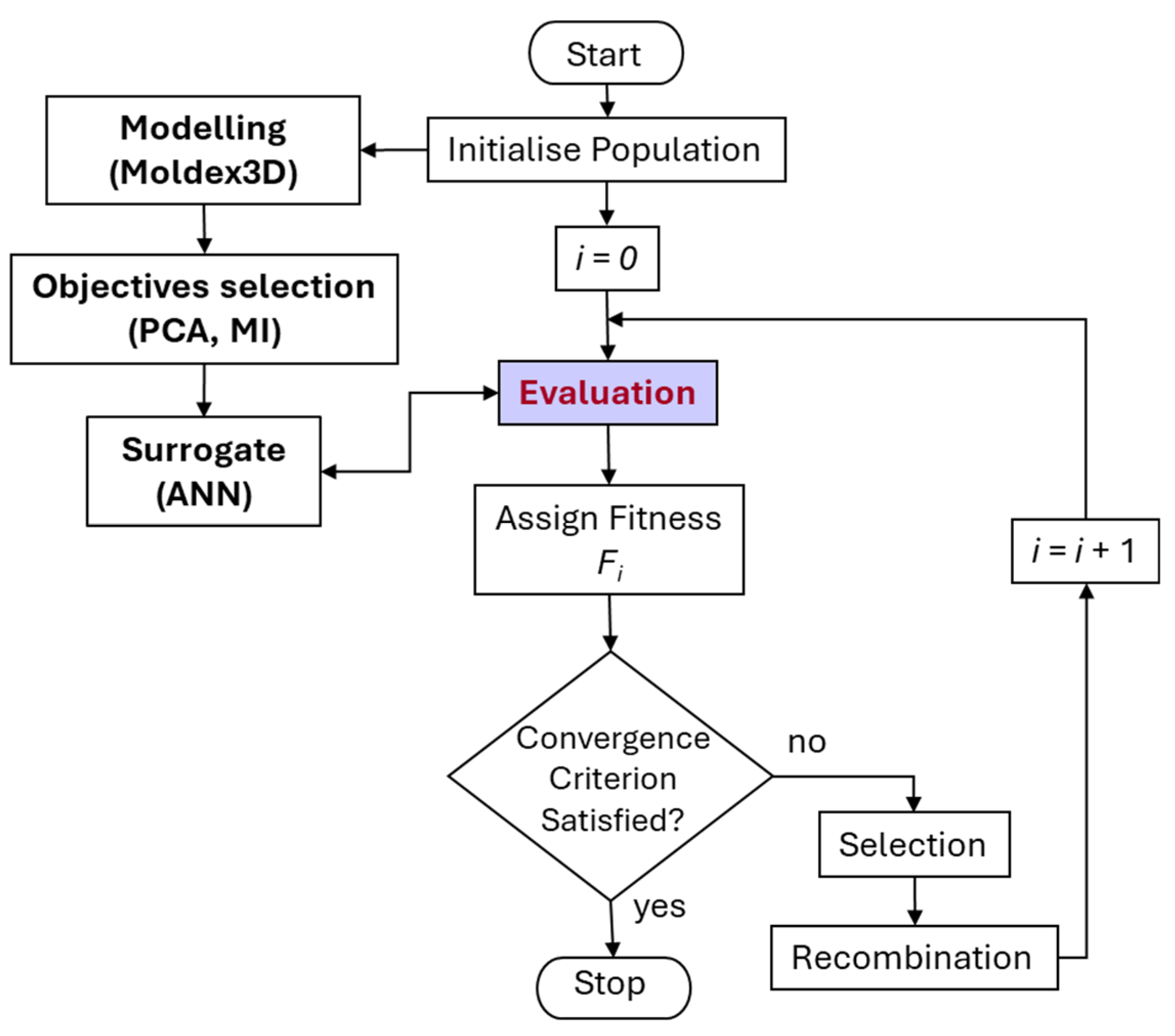
The approach applies objective selection through dimensionality-reduction techniques, trains artificial neural networks (ANNs) as surrogate models of the simulations, and then uses multi-objective evolutionary algorithms (MOEAs) to find optimal trade-offs. All steps are automated through Python scripts connected to the Moldex3D API, enabling efficient simulation, data handling, and optimization within a closed loop (
Figure 2). This strategy preserves accuracy while significantly reducing computational cost and allows the identification of cooling designs that balance cooling time, temperature uniformity, and part quality (Gaspar-Cunha et al., 2025a).
The overall workflow consists of the following main stages (
Figure 2):
Initial design generation and simulation: A set of initial mold designs is generated (randomly or via DOE) by varying cooling channel parameters. Each design is simulated in Moldex3D, and key outputs, including cooling time, temperature distribution, and warpage, are recorded.
Objective analysis and dimensionality reduction: Correlated objectives are analyzed using PCA, NL-PCA, MI/C, or kernel PCA to reduce them to a small number of representative components, typically retaining those explaining at least 95% of the variance.
Surrogate modeling with ANNs: Feed-forward ANNs are trained to predict the reduced objectives from design variables, replacing expensive simulations during optimization while maintaining high accuracy.
Multi-objective optimization: NSGA-II or NSGA-III is used to explore trade-offs among objectives using ANN predictions, efficiently identifying Pareto-optimal solutions.
Final verification: The best designs are re-simulated in Moldex3D to validate the surrogate-based results.
The Python-based integration of Moldex3D, dimensionality reduction, ANNs, and MOEAs enables an efficient and systematic search for high-performance conformal cooling channel designs.
3.2. Selection of Objectives
Injection molding simulations generate multiple quality indicators, including cooling efficiency, temperature uniformity, stresses, shrinkage, density, and warpage, resulting in 34 optimization objectives. Optimizing all of them simultaneously is computationally expensive due to strong redundancy and correlation, necessitating objective reduction.
To address this, the study applies Principal Component Analysis (PCA) and Non-Linear PCA (NL-PCA) to reduce dimensionality. PCA captures linear correlations, whereas NL-PCA better represents nonlinear relationships by mapping data into a higher-dimensional space prior to dimensionality reduction (Mukras et al., 2019; Smola & Schölkopf, 2004). In both cases, a small number of components (typically 2–3) can represent about 95% of the total variance, enabling efficient surrogate modeling with artificial neural networks (ANNs) and improving optimization convergence (Chang et al., 2023; Zhao & Cheng, 2016; Fernandes et al., 2012).
Because latent components can be difficult to interpret in industrial practice, an alternative objective-selection strategy was also implemented. Instead of transforming objectives, this approach selects a small subset of representative objectives while preserving their physical meaning. Redundancy is reduced by grouping highly dependent objectives using clustering based on nonlinear dependence measures such as Mutual Information, HSIC, or Variation of Information. From each group, one representative objective is selected to improve interpretability and computational efficiency (Chormunge & Jena, 2018).
In addition, Minimum Redundancy Maximum Relevance (mRMR) methods were used as a complementary selection strategy. In this unsupervised setting, objective relevance is measured using variance or entropy, while redundancy is quantified through pairwise dependence. Objectives are selected iteratively to maximize information gain while minimizing overlap with previously chosen ones (Peng et al., 2005).
Together, dimensionality reduction, clustering-based selection, and mRMR provide a robust framework for selecting informative and non-redundant objectives, improving efficiency and reliability in many-objective optimization of injection molding processes.
3.3. Strategy for Selecting a Reduced Number of Objectives
The clustering-based and mRMR-style methods described previously are applied across multiple parameter configurations, yielding several candidate objective subsets. To consolidate these results into a reduced subset for many-objective optimization, a consensus-based selection strategy is adopted.
Each objective is evaluated using two criteria: a consensus indicator, computed as the frequency with which it appears across candidate subsets (optionally weighted when user-defined objective weights are provided), and a redundancy indicator, computed as the average dependence on the objectives already selected. In this work, redundancy is quantified using signed Pearson correlation between objectives (after normalization) and updated iteratively as the subset grows.
The procedure starts with an initial “anchor” objective derived from the global dependency structure, then adds objectives sequentially by prioritizing high consensus and low redundancy, using a small tie-breaking/augmentation term to discriminate among near-equivalent candidates. To avoid selecting near-duplicates, objectives whose correlation with the selected set exceeds a threshold (0.95) are temporarily blocked; if all remaining candidates are blocked, the threshold is relaxed slightly to ensure progress. Because the relative importance of consensus versus redundancy depends on the intended application, a sensitivity grid is used to explore the hyperparameters controlling the emphasis on consensus (λ), redundancy (κ), and the tie-breaking term (μ). For each grid combination, the resulting subset and summary indicators (e.g., average normalized consensus and mean intra-subset correlation) are reported, enabling selection of the final configuration based on user preference.
3.4. Surrogate Models
This study uses artificial neural networks (ANNs) as surrogate models to approximate the relationship between mold design variables and performance objectives, avoiding the high computational cost of repeated Moldex3D simulations during optimization (Forrester et al., 2008; F. Liu et al., 2024).
A feedforward multilayer perceptron (MLP) is used, with inputs defined by cooling-channel parameters (e.g., diameter, spacing, number of channels) and outputs given by reduced objectives obtained using the techniques presented above. Training on simulation data allows the ANN to learn the complex nonlinear relationships between design variables and performance (Bishop, 1995). In particular, using ANN surrogates can significantly reduce the runtime per design iteration, potentially saving several hours of computational effort.
The data are split into training and validation sets, using mean squared error (MSE) as the loss function and optimizers such as SGD or Adam. Overfitting is controlled through early stopping and regularization (Bishop, 1995; Rasmussen & Williams, 2006). Hyperparameters are tuned using Bayesian optimization with the Tree-structured Parzen Estimator (TPE) from the Hyperopt library, which efficiently balances exploration and exploitation of the search space (Bergstra et al., 2011; Chen et al., 2010; Shahriari et al., 2016).
The hyperparameter search space considered in the Bayesian optimization is summarized in
Table 1. It covers network depth and width (number of hidden layers and neurons per layer), regularization (dropout), activation functions, optimizer type, learning rate, batch size, and the maximum number of training epochs. Each configuration is evaluated using cross-validation and normalized mean absolute error, and the best-performing setup is selected after multiple TPE evaluations. This Bayesian approach converges faster and more reliably than grid or random search, leading to robust and generalizable ANN models.
The trained ANNs achieve low prediction errors, typically only a few percent of the objective range, ensuring reliable approximation of simulation results (Q. Feng et al., 2020; Kurkin et al., 2021; Ma et al., 2023). This accuracy is essential, as poor surrogate models can misguide the optimizer (K. Deb et al., 2002).
By replacing expensive 3D thermal simulations with fast ANN predictions, population-based optimization methods such as MOEAs become computationally feasible (K. Deb et al., 2002; Kennedy & Eberhart, 1995). The ANN captures the key physical effects modeled in Moldex-3D, particularly the impact of cooling-channel geometry on part quality (Baruffa et al., 2024; S. Feng et al., 2021; Wilson et al., 2024), and is fully integrated into an automated Python-based simulation–optimization workflow.
3.5. Multi-Objective Optimization
In multi-objective optimization, a solution is evaluated across multiple conflicting objectives, typically expressed as a minimization problem:
where
is the feasible decision space and
maps to the objective space. The concept of
dominance defines the relative quality between solutions. A solution
dominates
(denoted
) if and only if:
A solution is considered optimal if no other solution improves one objective without worsening at least one other. The set of such solutions forms the Pareto front, which represents the best possible trade-offs. Multi-objective evolutionary algorithms (MOEAs) aim to approximate this front with solutions that are both accurate and well distributed (Coello et al., 2007; K. Deb, 2001).
Early MOEAs methods, such as VEGA and MOGA, relied on basic dominance concepts (Schaffer, 1985; Fonseca & Fleming, 1993). Later, second-generation algorithms such as NSGA-II and SPEA2 introduced elitism and efficient sorting, thereby improving convergence and diversity (K. Deb et al., 2002; Zitzler et al., 2001). More recent approaches include indicator-based and decomposition-based algorithms, as well as learning-assisted and interactive MOEAs, which focus on efficiency in complex problems (Beume et al., 2007; Jin, 2011; Zitzler & Künzli, 2004; Zhang & Li, 2007; D. Deb et al., 2014).
In this study, NSGA-II and NSGA-III are used because they are well-suited for engineering problems with conflicting objectives, such as cooling efficiency, temperature uniformity, and warpage in injection molding (Chang et al., 2023; Fernandes et al., 2010). NSGA-II is applied to two-objective problems, while NSGA-III is used when three or more objectives are considered, ensuring good solution diversity in higher-dimensional spaces (Deb et al., 2002, 2014; Mukras et al., 2019).
As referred to before, to reduce computational time, ANN surrogates are used to evaluate objectives quickly, making large-scale optimization feasible (Chang et al., 2023; Zhao & Cheng, 2016). Previous studies have shown that ANN-assisted MOEAs can reduce both warpage and cycle time (Kitayama et al., 2017; Lu & Huang, 2020).
4. Case Study
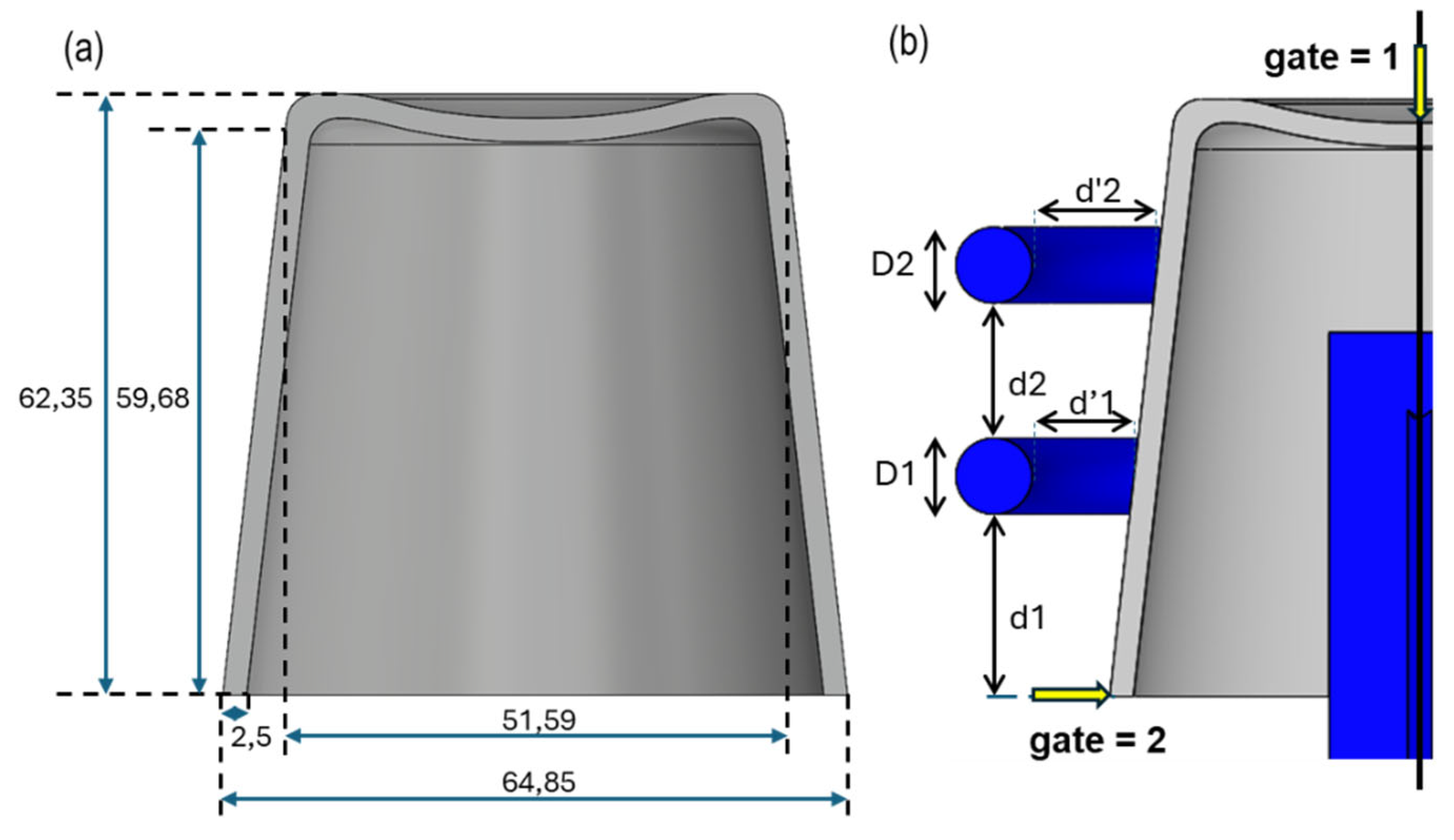
The mold used in this study, located at the university, produces a polymer cup and serves as a realistic test case for evaluating AI-based optimization methods in injection molding (
Figure 7a). It was chosen to balance sufficient geometric and thermal complexity with clear physical interpretation, making it suitable for validating the proposed methodology under practical conditions.
The mold has a conventional cooling system with circuits in both the fixed and movable halves to ensure proper thermal control and good part quality. The fixed side contains two independent circular cooling circuits with rectangular cross-sections, sealed with O-rings to promote stable and uniform cooling. The movable side employs a baffle-cooling system to enhance internal heat dissipation. In the original design, the gate is located at the base of the cup.
Two alternative gate configurations were analyzed (
Figure 3b). Gate 1 promotes more uniform filling and reduces weld lines and warpage, while Gate 2 creates bidirectional flow and visible weld lines. These configurations serve as a stress test for the cooling system and the surrogate models, enabling assessment of ANN performance under varying flow conditions.
As shown in
Figure 7b, two-ring conformal cooling channels (CCCs) were designed to comply with Moldex3D Studio API limitations and manufacturing constraints, including lateral channel entry and exit. The design variables and their allowed ranges are summarized in
Table 2.
The material used is Polypropylene BG055AI from Borealis AG, which is easy to process and well characterized. It has a melt flow rate of 22 g/10 min (230 °C/2.16 kg) and a recommended melt temperature of 220-250 °C. All processing parameters were fixed and standardized, as listed in
Table 3, to ensure that observed differences result only from cooling design and optimization strategies.
This case study investigates three main aspects: (i) the effect of gate location on the ability of the method to handle different initial temperature distributions; (ii) the impact of the number of initial designs (60, 160, and 300) on ANN performance; and (iii) the influence of different dimensionality reduction methods (PCA, NL-PCA, MI/C) on objective selection.
Overall, the study evaluates whether the proposed hybrid AI-based approach can manage the complexity of real injection molding optimization problems with high-dimensional and nonlinear objectives. The results aim to support practical guidelines for applying AI methods in industrial process optimization beyond injection molding.
The objectives were grouped into categories related to cooling efficiency and defect reduction to manage the complex effects caused by changes in the cooling system. Selection methods such as PCA, NL-PCA, and MI/Clustering were used to reduce the dataset and identify the most relevant objectives (
Table 4).
Temperature-based objectives focus on controlling temperature gradients inside the molded part, which strongly affect part quality. The analysis considers temperature differences through the part thickness, between the surface and core, and between opposite surfaces at the end of the cooling phase. To better target critical regions, the optimization emphasizes the 20% of areas with the highest temperature gradients, helping to reduce stresses and deformation.
Defect-based objectives address part quality using sixteen indicators. Warpage is evaluated using the maximum and minimum displacements along the X, Y, and Z directions, as well as the total deformation. Shrinkage is assessed by measuring volume changes in each direction and the overall volume. Separating maximum and minimum values helps detect asymmetries, which is important for nominally symmetric parts and for understanding the influence of flow direction.
Time-based objectives relate to production efficiency. Both the predefined cooling time and the cooling time predicted by Moldex3D are analyzed, allowing improvements in cycle time without reducing part quality.
Density and thermal efficiency objectives aim to ensure uniform material behavior. Density variation is quantified using the standard deviation to mitigate internal stresses and shrinkage. Thermal efficiency is evaluated by comparing heat transfer between fixed and movable cooling channels, thereby supporting improved energy efficiency and more uniform temperatures.
Von Mises stress objectives are used to assess mechanical performance. Maximum stress identifies critical zones, average stress represents overall behavior, and standard deviation indicates stress uniformity. These metrics help detect design weaknesses and improve part durability.
Based on these objectives, optimization was conducted to identify the optimal cooling configurations. The specific optimization cases are summarized in
Table 5. Final objective selection is performed by the decision maker (DM), supported by PCA, NL-PCA, and MI/Clustering methods.
5. Results and Discussion
5.1. An Illustrative Example
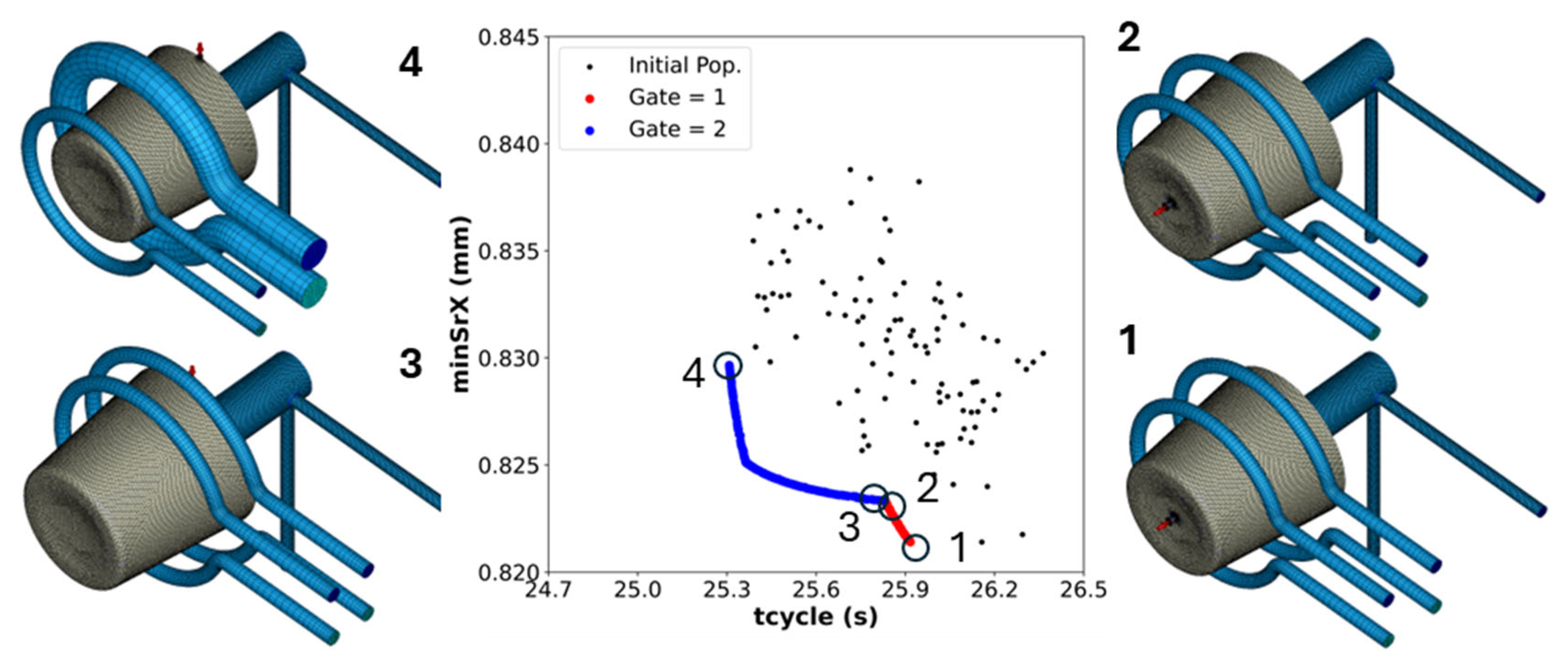
In this subsection, a bi-objective problem is considered in order to illustrate the complete workflow from dimensionality reduction to optimization and design interpretation. The two objectives are the cycle time of the process (tcycle) and the minimum shrinkage in the
-direction (
), representing productivity and dimensional stability, respectively. As shown in
Figure 5 (run 6), the DM selected this pair as a representative test case.
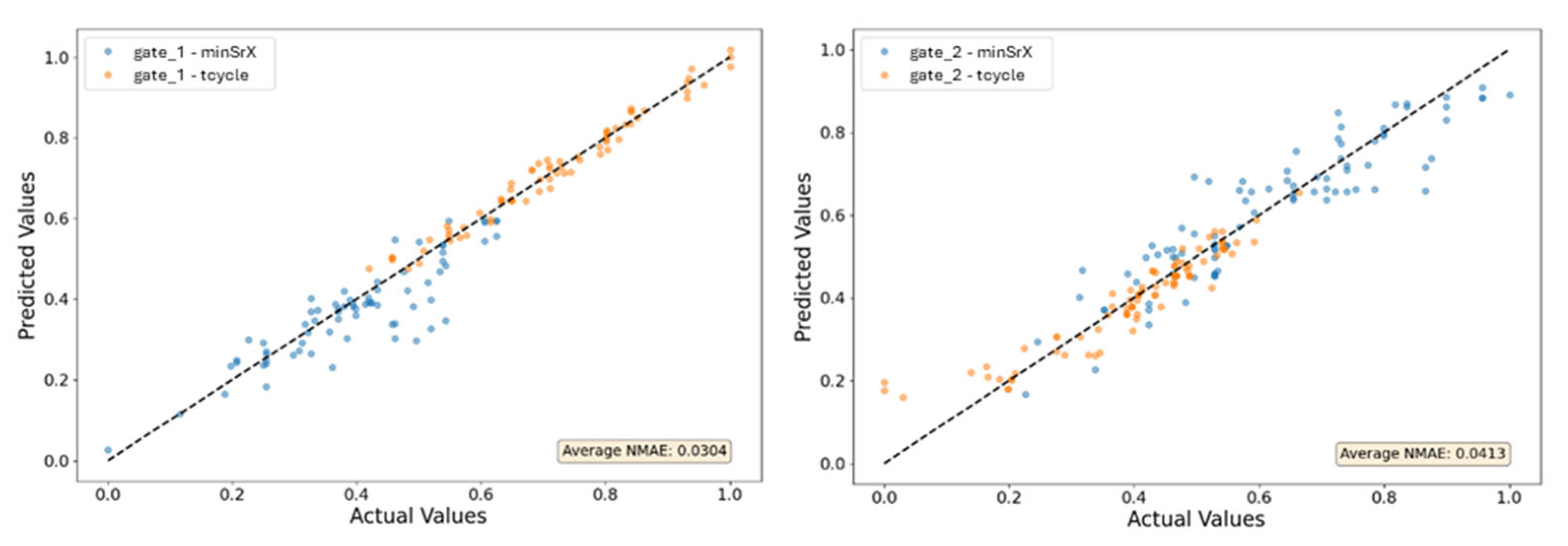
For each gate configuration (Gate 1 and Gate 2), separate feedforward ANN surrogate models were trained to approximate the two objectives using approximately 160 simulated data points.
Figure 4 shows the parity plots between the normalized predicted and actual values for both objectives and both gates. The points cluster closely around the diagonal, indicating a good agreement between simulations and surrogate predictions. The average normalized mean absolute error (NMAE) is approximately 0.030 for Gate 1 and 0.041 for Gate 2, confirming that the ANNs provide sufficiently accurate approximations to be used as cost-effective replacements for full injection-molding simulations in the subsequent runs. In the remainder of this paper, the ANN errors lie in the interval [0.0171; 0.0803].
The trained surrogates were then embedded in the multi-objective evolutionary algorithm to generate Pareto-optimal solutions in the (tcycle, minSrX) space.
Figure 5 displays the resulting fronts alongside the initial population, revealing distinct trade-off behaviors for the two gate locations. Generally, Gate 1 produces solutions with slightly lower shrinkage at the expense of longer cycle times. In contrast, Gate 2 accesses the region of highest productivity (shorter cycles) with a modest increase in shrinkage. To illustrate the physical implications of these results, four representative designs from the Gate 2 front (labeled 1–4) are highlighted. As the design progresses from Design 1 to Design 4, cycle time decreases while shrinkage gradually increases, reflecting the typical trade-off between productivity and dimensional accuracy.
Figure 5.
MOEA results for run 6 (
Table 4), tcycle versus minSrX: initial population (Gen. 1), Pareto front for Gates 1 and 2, and geometrical representation of four selected solutions.
Figure 5.
MOEA results for run 6 (
Table 4), tcycle versus minSrX: initial population (Gen. 1), Pareto front for Gates 1 and 2, and geometrical representation of four selected solutions.
The cooling-channel layouts associated with these four designs exhibit noticeable geometric differences that explain this performance shift. Design 1 employs thinner cooling channels, which moderate the heat-extraction rate; although this extends cycle time, it reduces internal stresses, thereby improving control over shrinkage. In contrast, Design 4 features larger-diameter channels strategically positioned to target critical heat accumulation zones, such as the cup’s bottom. This configuration maximizes heat removal efficiency, delivering the shortest cycle time but leading to slightly higher dimensional values. This example demonstrates how the proposed framework enables surrogate-based optimization to explore and visualize meaningful design trade-offs in a form directly interpretable to process engineers.
5.2. The Influence of Gate Location
To assess the robustness of the proposed methodology and to diversify the set of solutions, this study considers two distinct injection configurations. The gate location significantly alters the polymer melt flow and thermal history, resulting in a distinct defect pattern for each scenario.
Two gate locations were selected:
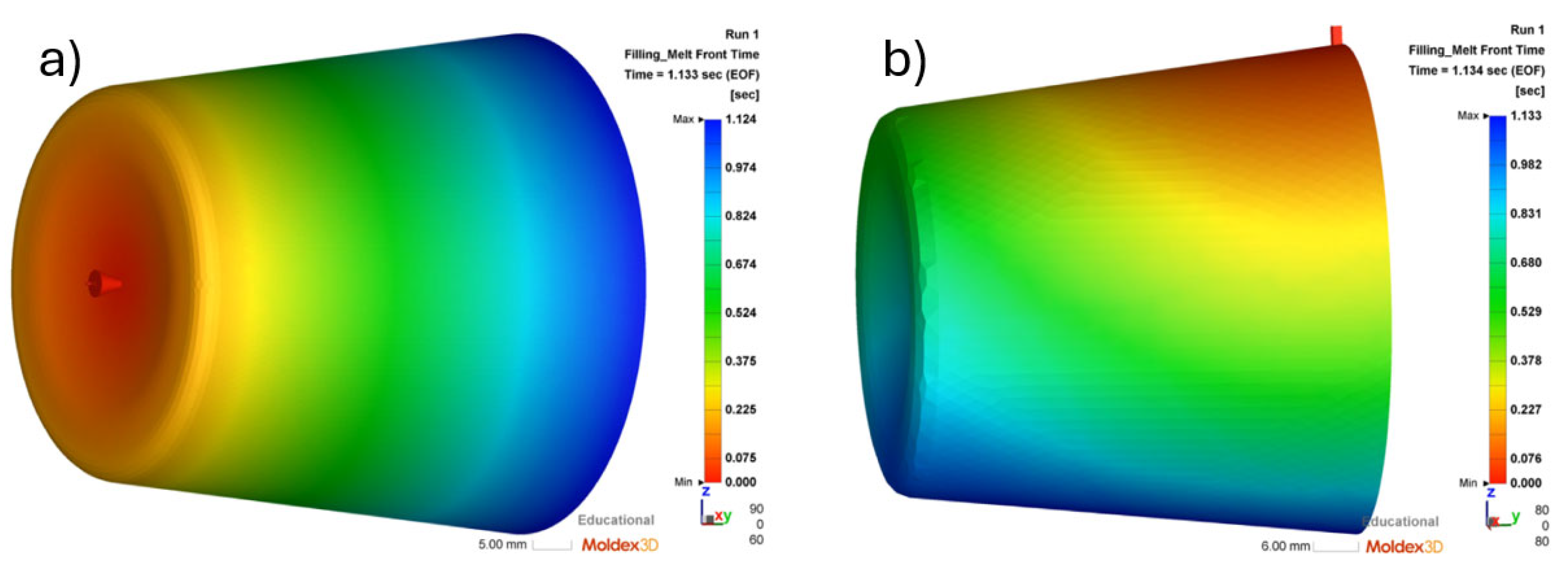
As illustrated in
Figure 6, melt-front propagation differs significantly between the two cases.
Figure 6a) shows a concentric filling pattern typical of a bottom gate, while
Figure 6b) demonstrates a transversal flow resulting from the side gate. Due to these physical discrepancies, the nonlinear relationships between the input variables and the objective functions differ fundamentally across the two gates.
Consequently, two independent Artificial Neural Networks (ANNs) were developed to accurately model the two gates.
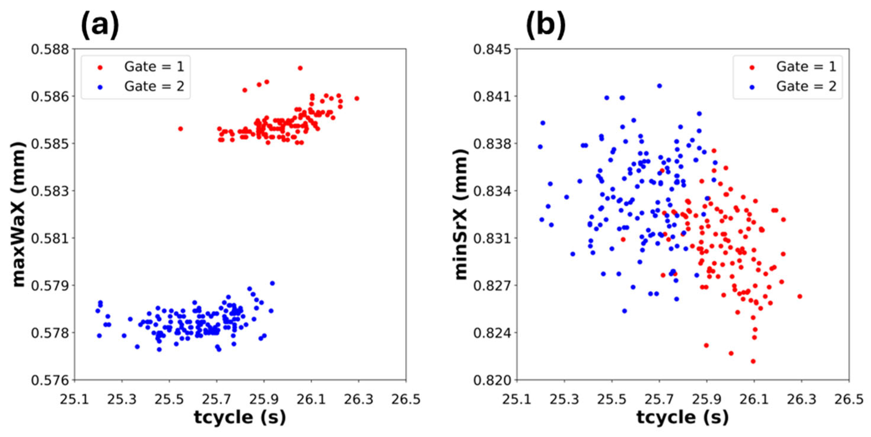
Figure 6 presents the scatter plots of the initial random populations used for training. A k-fold with five intervals and 60, 160, and 300 solutions was applied.
The solution spaces for Gate 1 (Red) and Gate 2 (Blue) are distinct. In
Figure 7a), the Gate 2 population clusters at significantly lower warpage values compared to Gate 1, suggesting an inherent advantage of the side-gate configuration for dimensional stability. This separation confirms that changing the gate location effectively diversifies the problem landscape, necessitating specific surrogate models for each dynamic.
Figure 7.
Scatter plots of the initial set of solutions used to train the ANN: (a) run 5; (b) run 6.
Figure 7.
Scatter plots of the initial set of solutions used to train the ANN: (a) run 5; (b) run 6.
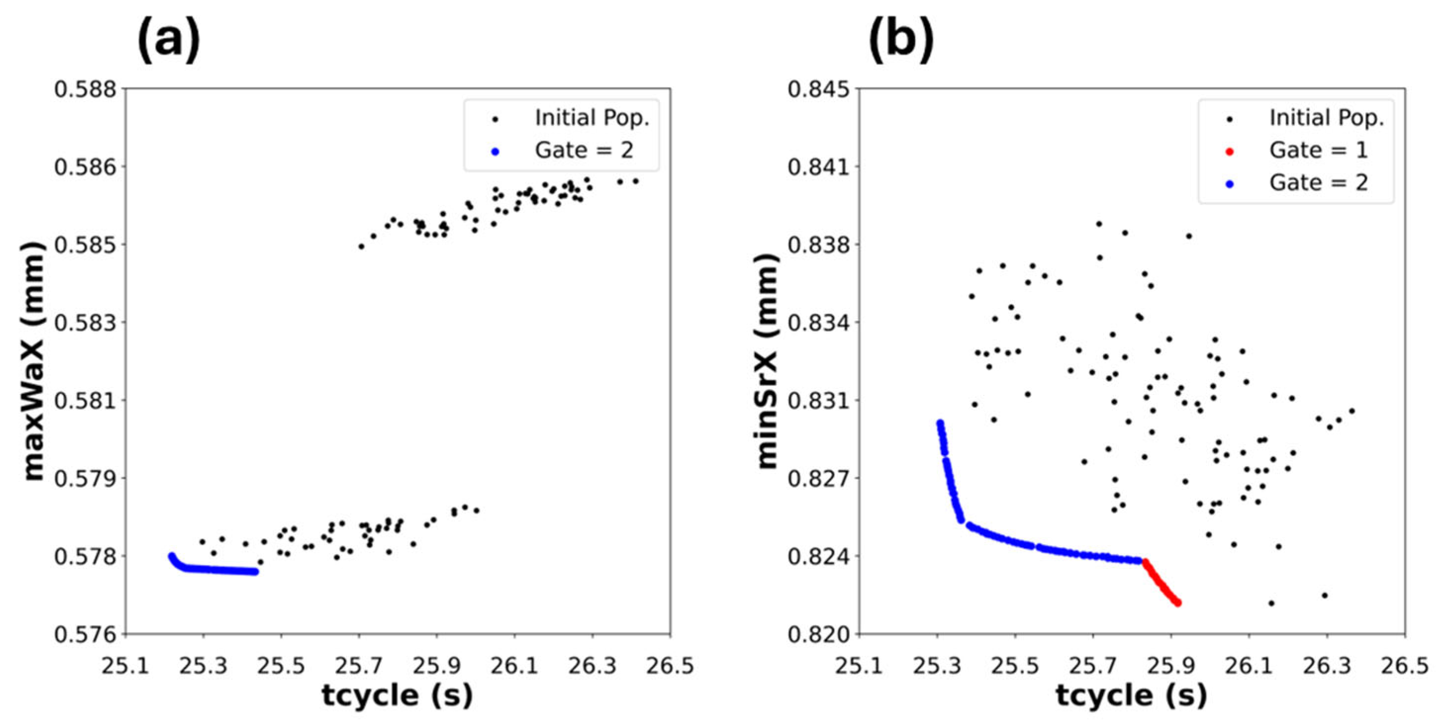
Finally, optimization was performed using the two ANNs simultaneously, treating the gate as an integer decision variable, with values 1 and 2 (see
Table 2).
Figure 8 displays the Pareto plots of this unified optimization approach, where black dots represent the initial population and colored points (Red for Gate 1, Blue for Gate 2) represent the identified non-dominated solutions.
The results demonstrate the methodology’s ability to converge to the minimization of objectives from widely dispersed populations. More importantly, the resulting fronts quantify the performance limits of each gate:
Warpage vs. Cycle Time (Figure 8a
): The side gate (Gate 2) yields significantly lower warpage. This is likely driven by transverse melt flow, which yields a more symmetric stress distribution along the X-axis compared with the complex radial stresses of the bottom gate.
Shrinkage vs. Cycle Time (Figure 8b
): A continuous Pareto front results. Gate 2 enables faster cycles (shorter cycle time) but with higher shrinkage, while the Gate 1 front extends into the region of longer cycle times to deliver minimum shrinkage.
5.3. Effect of the Number of Initial Solutions
5.3.1. Physical Consistency of the Results
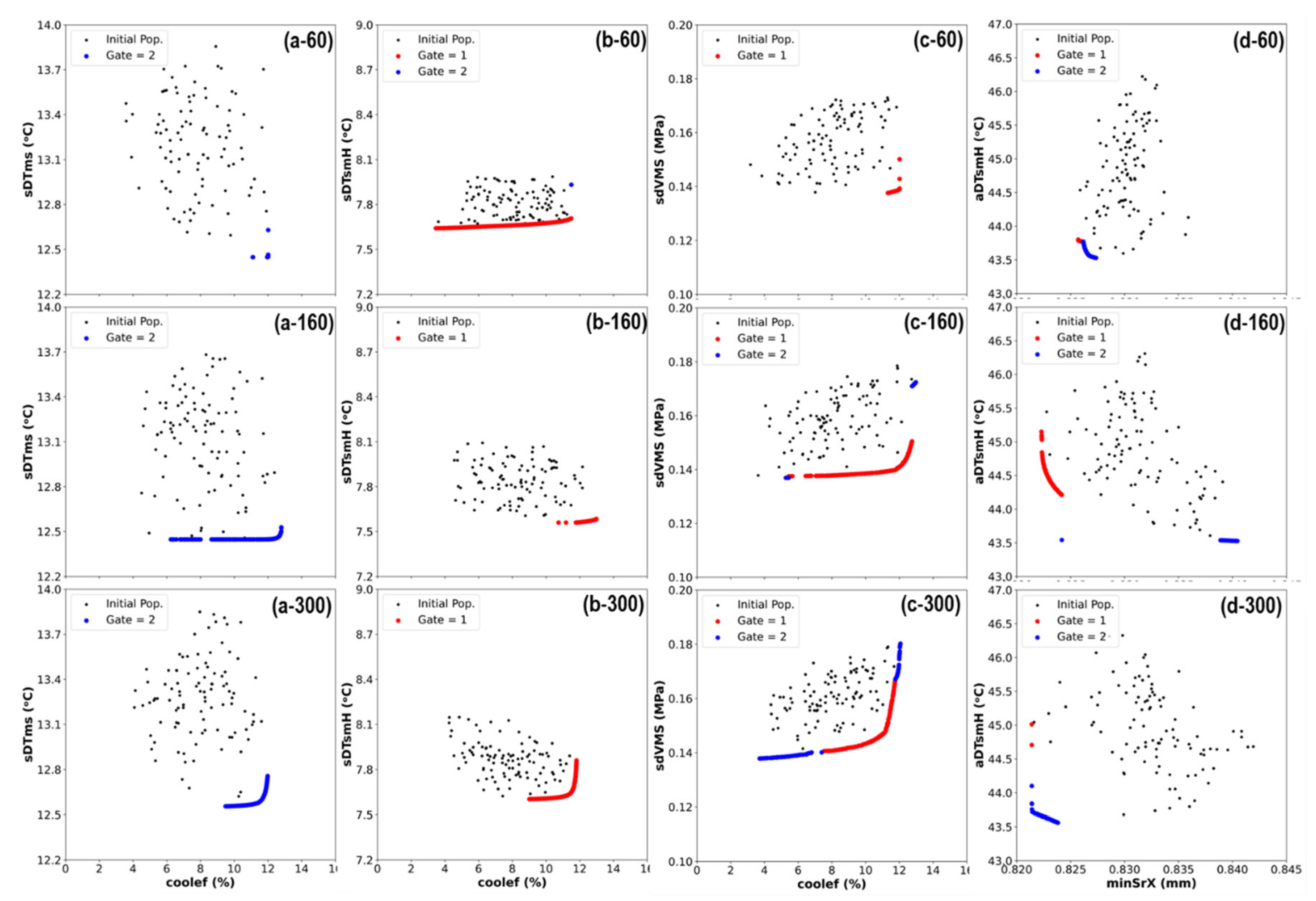
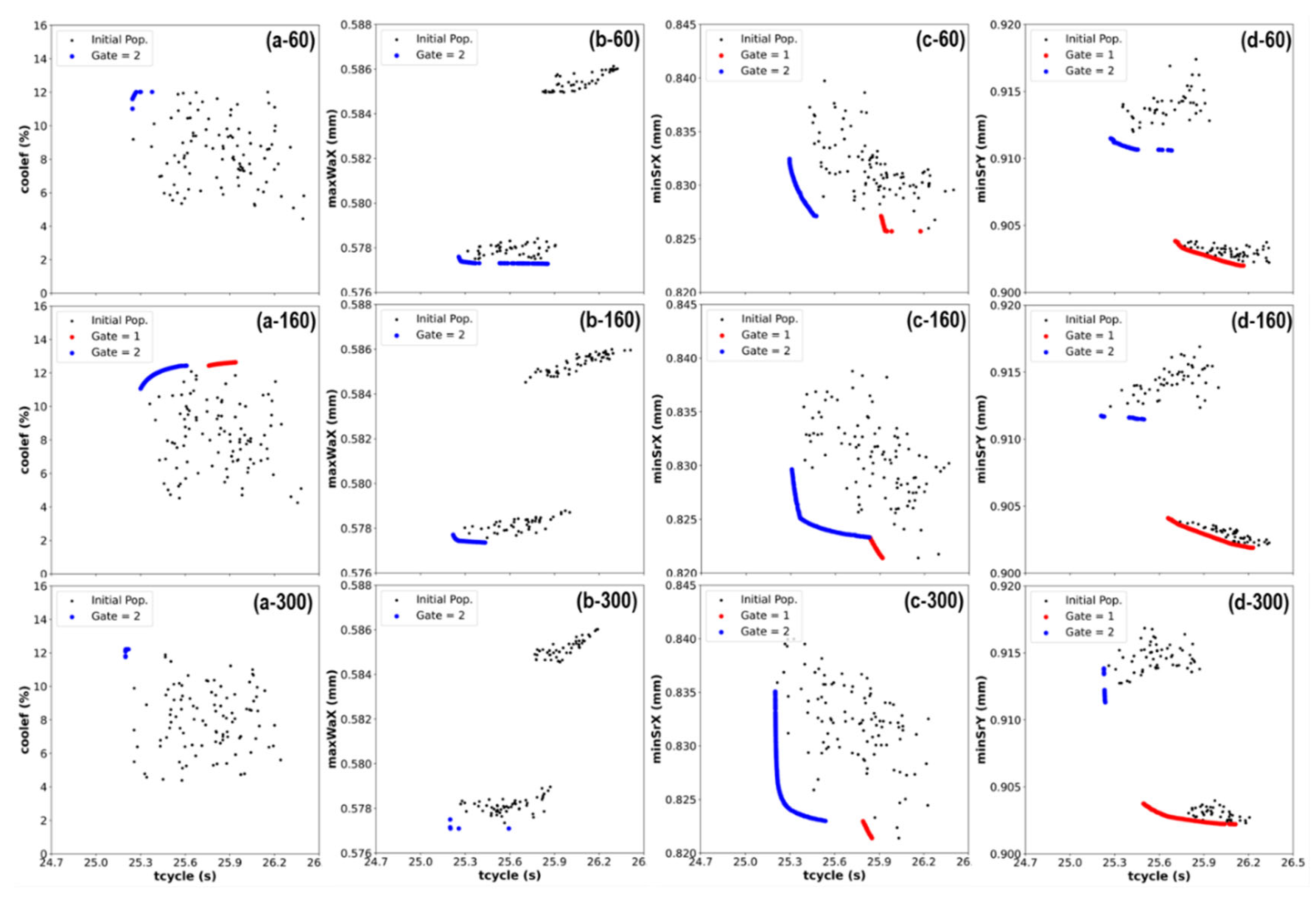
Before analyzing the statistical influence of the sampling density, it is essential to verify that the optimization results remain physically consistent across different numbers of initial solutions (N). Whether using 60, 160, or 300 simulations, the resulting Pareto fronts conform to the fundamental governing laws of polymer processing, as shown in
Figure 9 and
Figure 10. The conflict between objectives is evident in all cases, confirming that the algorithm is responding to physical phenomena rather than numerical noise:
Cycle Time vs. Thermal Homogeneity: In all datasets, a reduction in cycle time (tcycle) is consistently penalized by an increase in temperature standard deviation (sDTms). Physically, strictly limiting the cooling time prevents the uniform dissipation of heat, resulting in larger thermal gradients.
Cooling Efficiency vs. Shear Stress: Solutions that maximize cooling efficiency often require aggressive injection parameters or specific gate locations that induce higher shear rates (minSrX). The optimization consistently captures this trade-off, showing that thermal gains often come at the cost of mechanical stress.
Warpage vs. Productivity: The minimization of warpage (maxWaX) typically demands longer packing and cooling phases to ensure uniform shrinkage, which directly conflicts with maximizing productivity (minimizing tcycle).
5.3.2. Bi-Objective Optimization Runs
In the bi-objective optimization scenarios, as illustrated in
Figure 9 and
Figure 10, the impact of the initial population size is analyzed by observing the continuity and extension of the Pareto curves.
Low Density (N=60): The fronts are generally fragmented, presenting significant gaps between optimal solutions. The algorithm identifies the general trend but fails to populate the transition zones between conflicting objectives.
High Density (N=300): As expected, increasing the sample size to 300 typically results in the most continuous and smooth Pareto fronts. The “L-shape” of the trade-off is clearly defined, and the solutions extend further towards the asymptotes of the objective space.
Intermediate Density (N=160): While the general trend suggests that “more is better,” the improvement is not strictly linear across all objective pairs. In most cases, N=160 provides a significant improvement over N=60. However, in specific projections such as Shear Rate vs. Cycle Time (minSrX – tcycle), the configuration with 160 solutions yielded a remarkably well-defined and continuous front (
Figure 10, third column), in some aspects comparable to or even cleaner than the 300-solution optimizations. This suggests that, for specific physical interactions, a medium-density sampling is sufficient to capture the optimal boundary, and adding more points may yield only marginal density gains without extending the front.
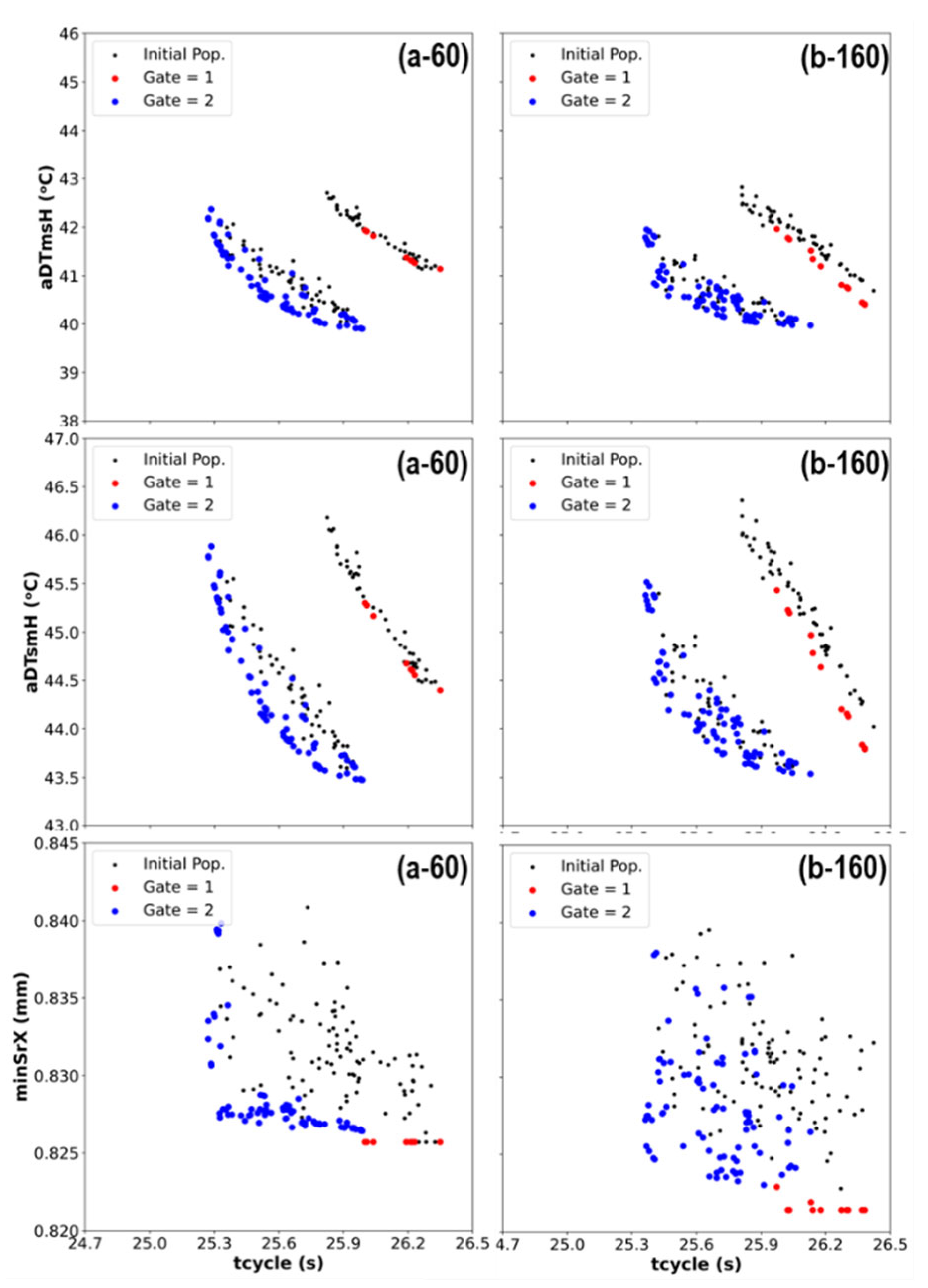
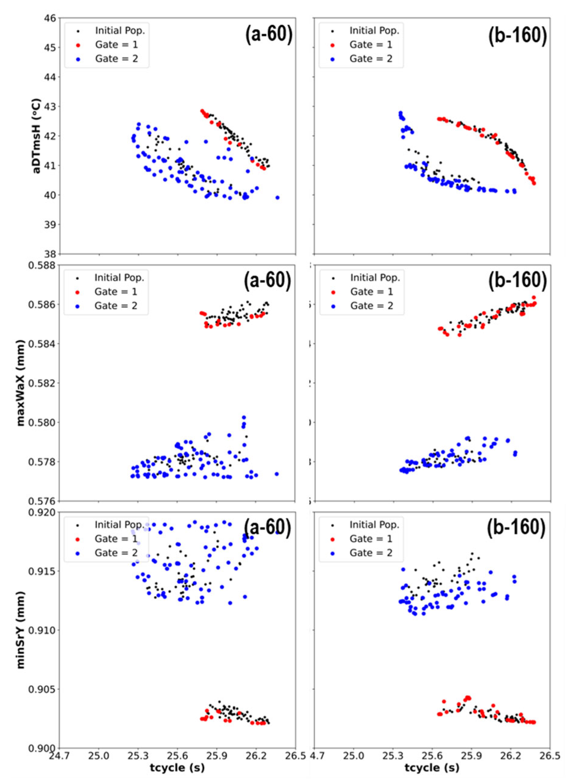
5.3.3. Four-Objective Optimization Runs
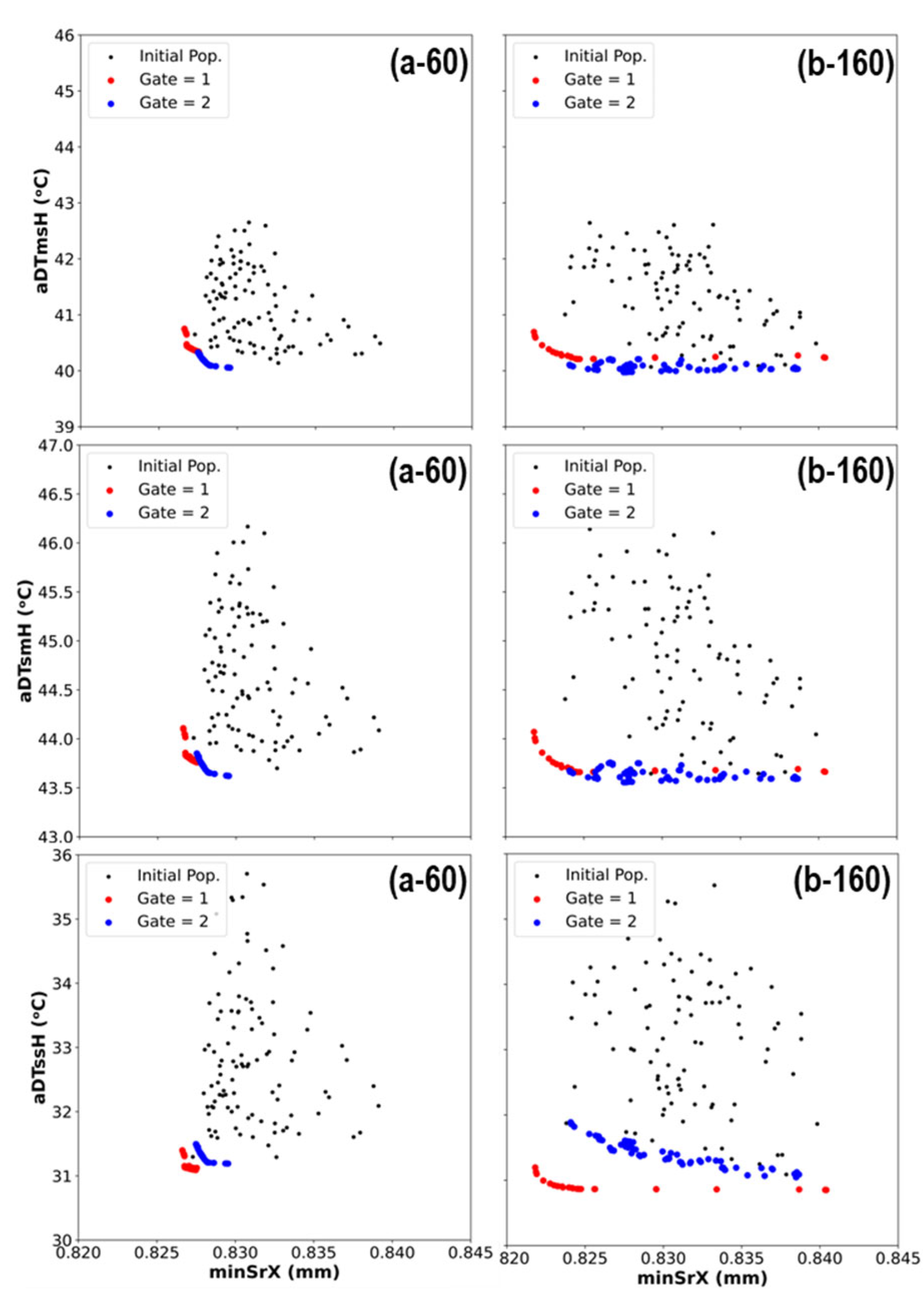
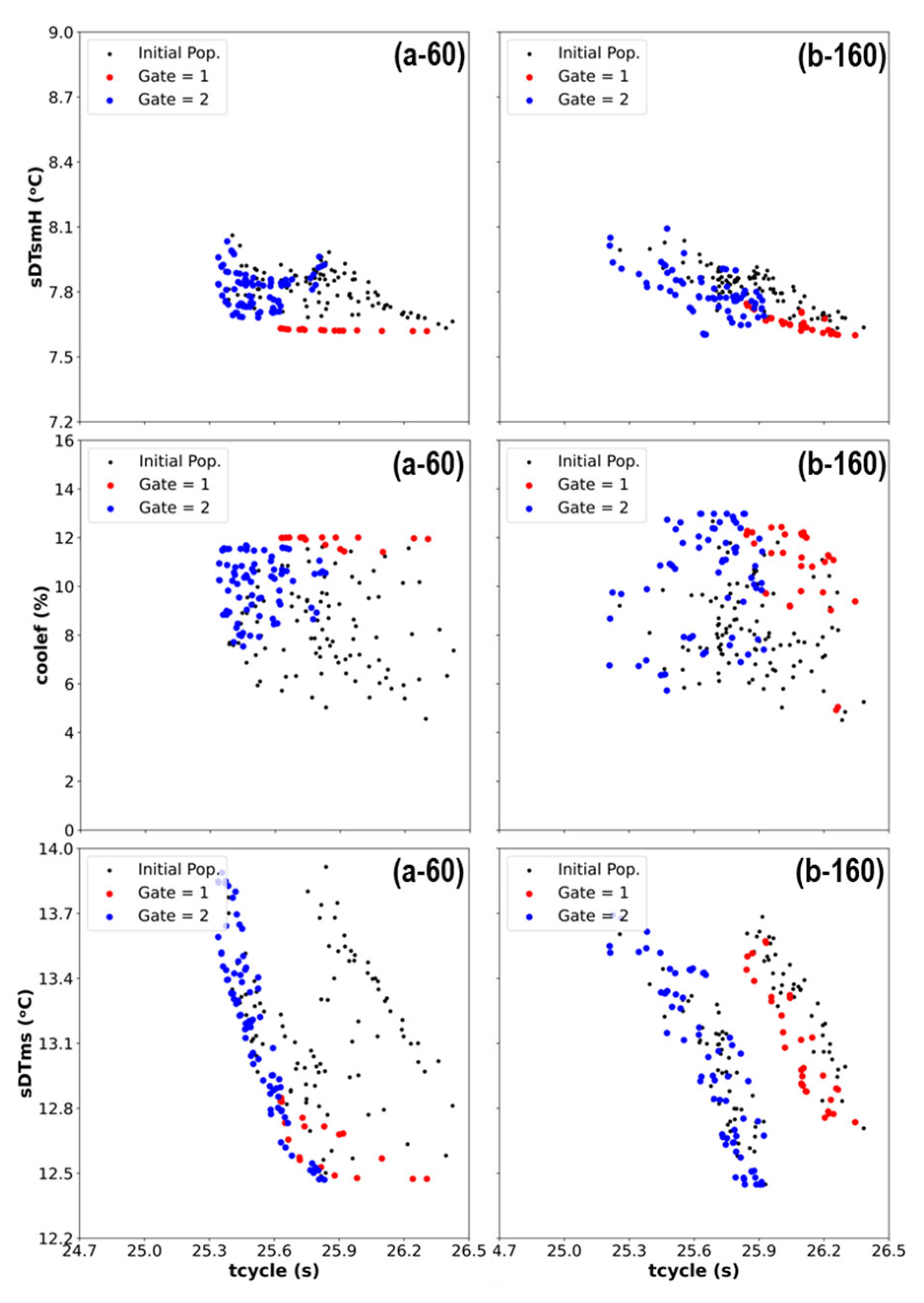
For the four-objective problems, the analysis requires interpreting 2D projections of a complex 4D hypersurface. Unlike the bi-objective cases, the solutions here manifest as scattered regions rather than distinct lines.
The interplay between Thermal Homogeneity and Cycle Time is a primary indicator of process quality, as shown in
Figure 11 and
Figure 12. Comparing the plots for N=60 and N=160 shows that the larger population size significantly shifts the “cloud” of solutions toward the bottom-left corner (the minimization region). The N=160 case successfully identifies solutions with lower cycle times that still maintain acceptable temperature deviations (aDTmsH), thereby revealing a high-performance region of the design space that remained largely unexplored in the N=60 case due to insufficient sampling.
When examining the mechanical constraints within the four-objective framework, specifically the Shear Rate (minSrX) projected against thermal indicators in
Figure 13, the complexity of the design space becomes evident. Since these plots represent 2D projections of a 4D hypersurface, the Pareto front manifests as a dispersed region rather than a single curve.
In the case with 60 initial solutions, this region appears as a sparse, disconnected cloud, providing limited insight into the actual Pareto front. However, increasing the population to 160 initial solutions significantly improves the solution density. This increased density reveals a clearer thick front, providing the designer with a continuum of valid choices rather than isolated points. Such density is crucial in multi-objective decision-making, as it allows for precise fine-tuning; for instance, one can select a specific Shear Rate limit and immediately observe the exact range of associated thermal penalties, which represents a level of detail that the sparse 60-solution dataset fails to provide.
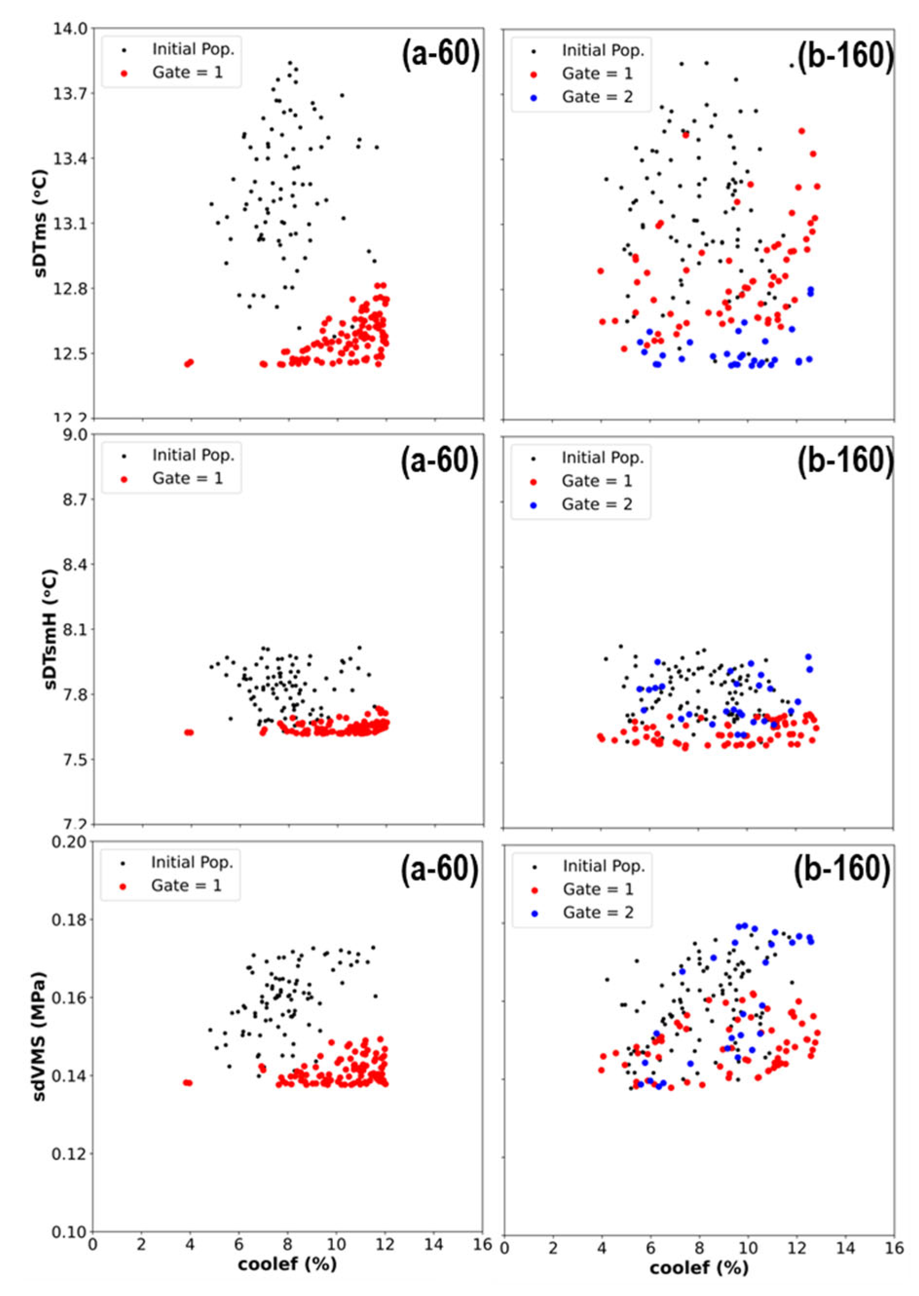
Finally, the optimization of Cooling Efficiency (coolef), as illustrated in
Figure 14 and
Figure 15, clearly demonstrates Pareto dominance. The fronts obtained with 160 solutions visually dominate those obtained with 60 solutions. This implies that, at the same level of cooling efficiency, the algorithm trained on a larger dataset identified gate configurations that yielded better performance across the remaining objectives (e.g., lower temperature variance), thereby validating the computational investment in the larger simulation set.
The comprehensive analysis of the initial sampling population size reveals a critical trade-off between computational cost and the fidelity of the optimization results. Based on the comparison between the cases using 60, 60, and 300 solutions, the following discussion is made:
Cost–fidelity trade-off: Increasing the initial sampling size generally produces denser Pareto fronts and can improve coverage near the extremes of the objective space. The transition from 60 to 160 initial solutions typically yields the most noticeable improvement in front density. At the same time, the gain from 160 to 300 is smaller and often exhibits diminishing returns relative to the additional computational effort.
Impact on decision-making: For early-stage exploration and constraint screening, 60 initial solutions already provide a meaningful set of trade-off solutions that support engineering insight and comparative decisions. Larger samples (160-300) primarily improve the front’s granularity, enabling finer adjustments among competing objectives when tight targets must be met (e.g., satisfying a specific mechanical limit with minimal impact on thermal performance).
Robustness and variability: Because the optimization process is stochastic, improvements with larger initial solutions are not uniform across all runs and objective regions. In practice, larger initial samples tend to reduce run-to-run variability and increase the likelihood of reaching more extreme trade-offs. In contrast, smaller samples may occasionally achieve comparable fronts at a fraction of the cost.
Therefore, the size of 60 initial solutions is sufficient for exploratory studies and time-constrained industrial settings, where a cost-effective yet informative approximation of the trade-offs is required; 160 is recommended when a denser and more robust front is needed for detailed design selection, and 300 is justified primarily for high-fidelity studies focused on accurately capturing the extreme regions of the Pareto front.
5.4. Effect of the Dimensionality Reduction Method
Dimensionality-reduction procedures do not modify the optimization algorithm itself, but they strongly influence which objectives are made available to the optimizer. Starting from the same set of 34 quality indicators, each method produces a reduced subset with a different emphasis on the underlying physical phenomena. The final subsets obtained in all optimizations are summarized in Table . When PCA is applied, the retained objectives correspond to those that contribute most strongly to the leading principal components. In the present case, PCA consistently selects indicators related to cooling performance (coolef) and temperature uniformity and stress (sDTms, sDTsmH, sdVMS), which together explain most of the variance in the original objective space. As a result, the reduced set focuses on the part’s global thermal and mechanical behavior, whereas other aspects, such as cycle time or local shrinkage, are not explicitly represented.
The NL-PCA configuration yields a different set of objectives. Because the latent structure is extracted in a non-linear feature space, back-projection onto the original indicators favors objectives that capture non-linear temperature differences and shrinkage (aDTsmH, aDTssH, aDTmsH, minSrX). In this case, the reduced set emphasises detailed thermal gradients and dimensional stability, whereas explicit measures of global cooling efficiency or warpage are omitted. The MI/C-based approach, which relies directly on mutual-information distances and clustering, tends to select at least one representative from each major group of correlated indicators (cooling efficiency, temperature uniformity, shrinkage/warpage and cycle time). In the present study, the final subset obtained with this method (run 14 in
Table 4) comprises the objectives aDTsmH, minSrX, coolef and sdVMS. This combination simultaneously captures non-linear temperature differences (aDTsmH), local shrinkage in the flow direction (minSrX), global cooling efficiency (coolef) and von Mises stress dispersion (sdVMS). Compared with PCA and NL-PCA, the MI/C configuration is less driven by total variance and more by informational diversity, favouring objectives that are weakly redundant with one another and preserving a broad coverage of the different physical phenomena involved in the process.
Therefore, the comparison shows that the choice of dimensionality-reduction method primarily determines which members of each correlated-objective family are retained in the reduced set. PCA emphasizes high-variance thermal and stress indicators; NL-PCA highlights non-linear temperature and shrinkage effects; and MI/C favors a more balanced, low-redundancy mix. Despite these differences, all methods consistently identify cooling performance, thermal homogeneity, and dimensional stability as key drivers of the process, indicating that the selection of physically meaningful objectives is robust with respect to the dimensionality reduction
6. Conclusions
A comparison of dimensionality-reduction methods shows that each approach places different emphasis on the physical phenomena represented in the reduced objective set. PCA primarily emphasizes high-variance thermal and stress indicators; NL-PCA highlights nonlinear temperature and shrinkage effects; and MI/C-based selection favors a low-redundancy combination that simultaneously covers cooling efficiency, temperature uniformity, and dimensional stability. Although all methods identify cooling performance and dimensional accuracy as key drivers, the MI/C configuration offers the most balanced and physically interpretable subset, which is advantageous for mitigating genetic bias by exposing the optimizer to diverse but non-redundant objectives.
The analysis of the number of initial solutions further illustrates the trade-off between search quality and computational cost. Increasing the initial sample from 60 to 160 and 300 designs produces, on average, progressively denser and slightly superior Pareto fronts, but at the price of a near-linear increase in simulation time (approximately one hour per design). However, in some optimization runs, a smaller initial sample yielded Pareto fronts comparable to, or even marginally better than, those obtained with a larger sample. This behavior is consistent with the stochastic nature of evolutionary algorithms and with genetic drift, whereby random fluctuations in the population may occasionally compensate for a reduced sampling density. These occasional inversions do not contradict the overall trend; instead, they indicate that beyond a certain number of initial solutions, the marginal benefits become small and are easily masked by stochastic effects. Consequently, a reduced initial sample of around 60 solutions appears to offer a more efficient compromise, yielding informative trade-offs while limiting the impact of genetic and surrogate bias within a feasible computational budget.
Given genetic bias in evolutionary search, improving the optimization process when surrogate models are employed is essential. The genetic operators and chromosome encoding tend to favor certain regions of the design space, which may lead to an over-representation of particular trade-off patterns and an under-exploration of others. When surrogate models are used as fitness evaluators, this algorithmic bias is compounded by the modelling bias of the surrogates themselves, making the choice of dimensionality-reduction strategy and initial sampling particularly critical.
The results indicate that controlling genetic bias in surrogate-assisted many-objective optimization cannot rely solely on the algorithm. The choice of dimensionality-reduction method and the allocation of the simulation budget (i.e., the number of initial solutions) play a decisive role in shaping the search space presented to the optimizer. Careful design of these components is therefore necessary to obtain Pareto fronts that are not only numerically competitive but also physically meaningful and robust for industrial decision-making.
Overall, the proposed methodology can be used to design CCC for injection molding and can be readily adapted to real-world, complex problems characterized by non-trivial relationships among DVs and objectives, and among objectives themselves when there are many objectives of different natures.
Author Contributions
“Conceptualization, A.G-C.; methodology, A.G-C., T.M., J.B.M.; software, T.M., J.B.M.; validation, T.M., J.B.M.; formal analysis, X.X.; investigation, X.X.; resources, A.J.P.; writing—original draft preparation, T.M., J.B.M.; writing—review and editing, A.G-C. and A.J.P.; .; supervision, A.G-C.; project administration, A.G-C and A.J.P.; funding acquisition, A.J.P.
Funding
This research was funded by FEDER funds through the COMPETE 2020 Program and National Funds through FCT (Portuguese Foundation for Science and Technology) under the projects UID-B/05256/2020 and UID-P/05256/2020.
Conflicts of Interest
The authors declare no conflicts of interest.
References
- Alam, K., & Kamal, M. R. (2003). A Genetic optimization of shrinkage by runner balancing. SPE Annual Technical Conference, 5, 639–641.
- Alam, K., & Kamal, M. R. (2004). Runner balancing by a direct genetic optimization of shrinkage. Polymer Engineering and Science, 44(10), 1949–1959. [CrossRef]
- Alam, K., & Kamal, M. R. (2005). A robust optimization of injection molding runner balancing. Comp. Chem. Eng., 29, 1934–1944.
- Baruffa, G., Pieressa, A., Sorgato, M., & Lucchetta, G. (2024). Transfer learning-based artificial neural network for predicting weld line occurrence through process simulations and molding trials. Journal of Manufacturing and Materials Processing, 8(3). [CrossRef]
- Bergstra, J., Bardenet, R., Bengio, Y., & Kégl, B. (2011). Algorithms for Hyper-Parameter Optimization. In J. Shawe-Taylor, R. Zemel, P. Bartlett, F. Pereira, & K. Q. Weinberger (Eds.), Advances in Neural Information Processing Systems (Vol. 24). Curran Associates, Inc. https://proceedings.neurips.cc/paper_files/paper/2011/file/86e8f7ab32cfd12577bc2619bc635690-Paper.pdf.
- Beume, N., Naujoks, B., & Emmerich, M. (2007). SMS-EMOA: Multiobjective selection based on dominated hypervolume. European Journal of Operational Research, 181, 1653–1669.
- Bishop, C. M. (1995). Neural networks for pattern recognition. Oxford University Press. [CrossRef]
- Brooks, H., & Brigden, K. (2016). Design of conformal cooling layers with self-supporting lattices for additively manufactured tooling. Additive Manufacturing, 11, 16–22. [CrossRef]
- Chang, H., Sun, Y., Wang, R., & Lu, S. (2023). Application of the NSGA-II algorithm and kriging model to optimise the process parameters for the improvement of the quality of fresnel lenses. Polymers, 15(16). [CrossRef]
- Chen, W., Zhou, X. H., Wang, H. F., & Wang, W. (2010). Multi-objective optimal approach for injection molding based on surrogate model and particle swarm optimization algorithm. Journal of Shanghai Jiaotong University (Science), 15(1), 88–93. [CrossRef]
- Chormunge, S., & Jena, S. (2018). Correlation based feature selection with clustering for high dimensional data. Journal of Electrical Systems and Information Technology, 5(3), 542–549. [CrossRef]
- Chung, K., & Das, S. (2018). Additive manufacturing of conformal cooling channels for injection mold tools: Current progress and challenges. Additive Manufacturing, 21, 672–686.
- Coello, C. A. C., Lamont, G. B., & Van Veldhuizen, D. A. (2007). Evolutionary algorithms for solving multi-objective problems. Springer. [CrossRef]
- Deb, D., Jain, A., & Singh, R. K. (2014). An evolutionary many-objective optimization algorithm using reference-point-based nondominated sorting approach, part I: Solving problems with box constraints. IEEE Transactions on Evolutionary Computation, 18(4), 577–601. [CrossRef]
- Deb, K. (2001). Multi-objective optimization using evolutionary algorithms. Wiley.
- Deb, K., Pratap, A., Agarwal, S., & Meyarivan, T. (2002). A fast and elitist multi-objective genetic algorithm: NSGA-II. IEEE Transactions on Evolutionary Computation, 6(2), 182–197. [CrossRef]
- Eiamsa-Ard, K., & Wannissorn, K. (2015). Conformal bubbler cooling for molds by metal deposition process. CAD Computer Aided Design, 69, 126–133. [CrossRef]
- Faes, A. G. (2000). Injection Molding Handbook. Hanser Gardner Publications.
- Feng, Q., Liu, L., & Zhou, X. (2020). Automated multi-objective optimization for thin-walled plastic products using Taguchi, ANOVA, and hybrid ANN-MOGA. The International Journal of Advanced Manufacturing Technology, 106(1–2), 559–575. [CrossRef]
- Feng, Q. Q., & Zhou, X. (2019). Automated and robust multi-objective optimal design of thin-walled product injection process based on hybrid RBF-MOGA. International Journal of Advanced Manufacturing Technology, 101(9–12), 2217–2231. [CrossRef]
- Feng, S., Kamat, A. M., & Pei, Y. (2021). Design and fabrication of conformal cooling channels in molds: Review and progress updates. International Journal of Heat and Mass Transfer, 171, 121082. [CrossRef]
- Fernandes, C., Pontes, A. J., Viana, J. C., & Gaspar-Cunha, A. (2010). Using multiobjective evolutionary algorithms in the optimization of operating conditions of polymer injection molding. Polymer Engineering and Science, 50(8), 1667–1678. [CrossRef]
- Fernandes, C., Pontes, A. J., Viana, J. C., & Gaspar-Cunha, A. (2012). Using multi-objective evolutionary algorithms for optimization of the cooling system in polymer injection molding. Int. Polym. Proc., 27, 213–223. [CrossRef]
- Ferreira, I., Weck, O. De, Saraiva, P., & Cabral, J. (2010). Multidisciplinary optimization of injection molding systems. Structural and Multidisciplinary Optimization, 41, 621–635. [CrossRef]
- Fonseca, C. M., & Fleming, P. J. (1993). Genetic Algorithms for Multiobjective Optimization: FormulationDiscussion and Generalization. International Conference on Genetic Algorithms. https://api.semanticscholar.org/CorpusID:7129189.
- Forrester, A., Sobester, A., & Keane, A. J. (2008). Engineering design via surrogate modelling: A practical guide. Wiley. [CrossRef]
- Gao, Z., Dong, G., Tang, Y., & Zhao, Y. F. (2023). Machine learning aided design of conformal cooling channels for injection molding. Journal of Intelligent Manufacturing, 34(3), 1183–1201. [CrossRef]
- Gaspar-Cunha, A., Melo, J., Marques, T., & Pontes, A. (2025a). A Review on Injection Molding: Conformal Cooling Channels, Modelling, Surrogate Models and Multi-Objective Optimization. Polymers, 17(7), 919. [CrossRef]
- Gaspar-Cunha, A., Melo, J., Marques, T., & Pontes, A. (2025b). Application of artificial intelligence techniques to select the objectives in the multi-objective optimization of injection molding. International Polymer Processing. [CrossRef]
- Gaspar-Cunha, A., & Viana, J. (2005). Using multi-objective evolutionary algorithms to optimize mechanical properties of injection molded part. Int. Polym. Process., 20, 274–285.
- Goodship, V. (2017). Injection molding: A practical guide. Smithers Rapra.
- Hashimoto, S., Kitayama, S., Takano, M., Kubo, Y., & Aiba, S. (2020). Simultaneous optimization of variable injection velocity profile and process parameters in plastic injection molding for minimizing weldline and cycle time. Journal of Advanced Mechanical Design, Systems and Manufacturing, 14(3), 1881–3054. [CrossRef]
- Hsu, F. H., Wang, K., Huang, C. T., & Chang, R. Y. (2013). Investigation on conformal cooling system design in injection molding. Advances in Production Engineering & Management, 8(2), 107–115. [CrossRef]
- Jahan, S. A., Wu, T., Zhang, Y., El-Mounayri, H., Tovar, A., Zhang, J., Acheson, D., Nalim, R., Guo, X., & Lee, W. H. (2016). Implementation of Conformal Cooling & Topology Optimization in 3D Printed Stainless Steel Porous Structure Injection Molds. Procedia Manufacturing, 5, 901–915. [CrossRef]
- Jahan, S. A., Wu, T., Zhang, Y., Zhang, J., Tovar, A., & Elmounayri, H. (2017). Thermo-mechanical design optimization of conformal cooling channels using design of experiments approach. Procedia Manufacturing, 10, 898–911. [CrossRef]
- Jahan, S., Wu, T., Shin, Y., Tovar, A., & El-Mounayri, H. (2019). Thermo-fluid topology optimization and experimental study of conformal cooling channels for 3D printed plastic injection molds. Procedia Manufacturing, 34, 631–639. [CrossRef]
- Jin, Y. (2011). Surrogate-assisted evolutionary computation: Recent advances and future challenges. Swarm and Evolutionary Computation, 1(2), 61–70.
- Jolliffe, I. T., & Cadima, J. (2016). Principal component analysis: a review and recent developments. Philosophical Transactions of the Royal Society A: Mathematical, Physical and Engineering Sciences, 374(2065).
- Kanbur, B. B., Zhou, Y., Shen, S., & Duan, F. (2020). Neural network-integrated multiobjective optimization of 3D-printed conformal cooling channels. IEEE Xplore. [CrossRef]
- Kanbur, B. B., Zhou, Y., Shen, S., Wong, K. H., Chen, C., Shocket, A., & Duan, F. (2022). Metal additive manufacturing of conformal cooling channels in plastic injection molds with high number of design variables. Materials Today: Proceedings, 70, 541–547. [CrossRef]
- Kariminejad, M., Tormey, D., Ryan, C., O’Hara, C., Weinert, A., & McAfee, M. (2024). Single and multi-objective real-time optimisation of an industrial injection moulding process via a bayesian adaptive design of experiment approach. Scientific Reports, 14, 1. [CrossRef]
- Kennedy, J., & Eberhart, R. (1995). Particle swarm optimization. Proceedings of ICNN’95 - International Conference on Neural Networks, 4, 1942–1948. [CrossRef]
- Kim, J., & Lee, S. (2019). Intelligent design optimization of conformal cooling channels for plastic injection molding. Journal of Computational Design and Engineering, 6(2), 161–168.
- Kitayama, S., Miyakawa, H., Takano, M., & Aiba, S. (2017). Multi-objective optimization of injection molding process parameters for short cycle time and warpage reduction using conformal cooling channel. International Journal of Advanced Manufacturing Technology, 88(5–8), 1735–1744. [CrossRef]
- Kitayama, S., Tamada, K., Takano, M., & Aiba, S. (2018). Numerical optimization of process parameters in plastic injection molding for minimizing weldlines and clamping force using conformal cooling channel. Journal of Manufacturing Processes, 32, 782–790. [CrossRef]
- Konuskan, Y., Yılmaz, A. H., Tosun, B., & Lazoglu, I. (2023). Machine learning-aided cooling profile prediction in plastic injection molding. International Journal of Advanced Manufacturing Technology, 2957–2968. [CrossRef]
- Kurkin, E., Kishov, E., Barcenas, O. U. E., & Chertykovtseva, V. (2021). Gate location optimization of injection molded aerospace brackets using metaheuristic algorithms. 2021 International Scientific and Technical Engine Conference, EC 2021, 1–6. [CrossRef]
- Le Goff, R., & Garcia, D. (2011). Multi-objective optimization strategy for the design of injection mold cooling system. Society of Plastics Engineers - EUROTEC 2011 Conference Proceedings, March.
- Liu, F., Pang, J., & Xu, Z. (2024). Multi-objective optimization of injection molding process parameters for moderately thick plane lens based on PSO-BPNN, OMOPSO, and TOPSIS. Processes, 12(1). [CrossRef]
- Liu, X., Fan, X., Guo, Y., Liu, Z., & Ding, W. (2022). Quality monitoring and multi-objective optimization of the glass fiber-reinforced plastic injection molded products. SAE International Journal of Materials and Manufacturing, 16(1). [CrossRef]
- Lu, Y., & Huang, H. (2020). Multi-objective optimization of injection process parameters based on EBFNN and NSGA-II. Journal of Physics: Conference Series, 1637(1). [CrossRef]
- Ma, Y., Dang, K., Wang, X., Zhou, Y., Yang, W., & Xie, P. (2023). Intelligent recommendation system of injection molding process parameters based on CAE simulation, process window and machine learning. The International Journal of Advanced Manufacturing Technology, 128(9–10), 4703–4716. [CrossRef]
- Mazur, M., Brincat, P., Leary, M., & Brandt, M. (2017). Numerical and experimental evaluation of a conformally cooled H13 steel injection mould manufactured with selective laser melting. International Journal of Advanced Manufacturing Technology, 93(1–4), 881–900. [CrossRef]
- Menges, G., Rosato, D. V., & Rosato, D. V. (2001). Injection molding handbook. Kluwer Academic Publishers.
- Mukras, S. M. S. (2020). Experimental-based optimization of injection molding process parameters for short product cycle time. Advances in Polymer Technology, 2020. [CrossRef]
- Mukras, S. M. S., Omar, H. M., & Al-Mufadi, F. A. (2019). Experimental-based multi-objective optimization of injection molding process parameters. Arabian Journal for Science and Engineering, 44(9), 7653–7665. [CrossRef]
- Nguyen, V.-T., Minh, P. S., Uyen, T. M. T., Do, T. T., Ha, N. C., & Nguyen, V. T. T. (2023). Conformal cooling channel design for improving temperature distribution on the cavity surface in the injection molding process. Polymers, 15(13), 2793.
- Osswald, T. A., & Hernández-Ortiz, J. P. (2006). Polymer processing: Modeling and simulation. Hanser.
- Peng, H., Long, F., & Ding, C. (2005). Feature selection based on mutual information criteria of max-dependency, max-relevance, and min-redundancy. IEEE Transactions on Pattern Analysis and Machine Intelligence, 27(8), 1226–1238. [CrossRef]
- Rasmussen, C. E., & Williams, C. K. I. (2006). Gaussian processes for machine learning. MIT Press. [CrossRef]
- Rosato, D. V, & et al. (2007). Injection Molding Handbook.
- Saifullah, A. B. M., Masood, S. H., & Sbarski, I. (2012). Thermal-structural analysis of bi-metallic conformal cooling for injection moulds. International Journal of Advanced Manufacturing Technology, 62(1–4), 123–133. [CrossRef]
- Schaffer, J. (1985). Multiple Objective Optimization with Vector Evaluated Genetic Algorithms. In Proceedings of the First Int. Conference on Genetic Algortihms, Ed. G.J.E Grefensette, J.J. Lawrence Erlbraum.
- Shahriari, B., Swersky, K., Wang, Z., Adams, R. P., & de Freitas, N. (2016). Taking the human out of the loop: A review of Bayesian optimization. Proceedings of the IEEE, 104(1), 148–175. [CrossRef]
- Shen, S., Kanbur, B. B., Zhou, Y., & Duan, F. (2019). Thermal and mechanical analysis for conformal cooling channel in plastic injection molding. Materials Today: Proceedings, 28(xxxx), 396–401. [CrossRef]
- Silva, H. M., Noversa, J. T., Fernandes, L., Rodrigues, H. L., & Pontes, A. J. (2022). Design, simulation and optimization of conformal cooling channels in injection molds: a review. In International Journal of Advanced Manufacturing Technology (Vol. 120, Issues 7–8, pp. 4291–4305). Springer Science and Business Media Deutschland GmbH. [CrossRef]
- Smola, A. J., & Schölkopf, B. (2004). A tutorial on support vector regression. Statistics and Computing, 14(3), 199–222. [CrossRef]
- Tuteski, O., & Kočov, A. (2018). Conformal cooling channels in injection molding tools – design considerations. Int. Sci. Congr. Mach. Technol. Mater., 12(11), 445–448.
- van As, B., Combrinck, J., Booysen, G. J., & de Beer, D. J. (2017). Direct metal laser sintering, using conformal cooling, for high volume production tooling. South African Journal of Industrial Engineering, 28(4), 170–182. [CrossRef]
- Wang, D., Fan, X., Guo, Y., Lu, X., Wang, C., & Ding, W. (2022). Quality prediction and control of thin-walled shell injection molding based on GWO-PSO, ACO-BP, and NSGA-II. Journal of Polymer Engineering, 42(9), 876–884. [CrossRef]
- Wei, Z., Wu, J., Shi, N., & Li, L. (2020). Review of conformal cooling system design and additive manufacturing for injection molds. Mathematical Biosciences and Engineering, 17(5), 5414–5431. [CrossRef]
- Wilson, N., Gupta, M., Patel, M., Mazur, M., Nguyen, V., Gulizia, S., & Cole, I. (2024). Generative design of conformal cooling channels for hybrid-manufactured injection moulding tools. International Journal of Advanced Manufacturing Technology, 133(1–2), 861–888. [CrossRef]
- Wu, T., & Tovar, A. (2018). Design for additive manufacturing of conformal cooling channels using thermal-fluid topology optimization and application in injection molds. Proceedings of the ASME Design Engineering Technical Conference, 2B-2018. [CrossRef]
- Xu, G., Yang, Z., & Long, G. (2012). Multi-objective optimization of MIMO plastic injection molding process conditions based on particle swarm optimization. Int. J. Adv. Manuf. Technol., 58, 521–531.
- Zacharski, A., Samborski, T., Zbrowski, A., Kozioł, S., & Poszwa, P. (2023). Modular injection mould with a conformal cooling channel for the production of hydraulic filter housings. Technologia i Automatyzacja Montażu, 122(4), 48–55. [CrossRef]
- Zeng, W., Yi, G., Zhang, S., & Wang, Z. (2024). Multi-objective optimization method of injection molding process parameters based on hierarchical sampling and comprehensive entropy weights. International Journal of Advanced Manufacturing Technology, 133(3–4), 1481–1499. [CrossRef]
- Zhai, M., Lam, Y. C., & Au, C. K. (2009). Runner sizing in multiple cavity injection mould by non-dominated sorting genetic algorithm. Engineering with Computers, 25(3), 237–245. [CrossRef]
- Zhang, Q., & Li, H. (2007). MOEA/D: A multiobjective evolutionary algorithm based on decomposition. IEEE Transactions on Evolutionary Computation, 11(6), 712–731.
- Zhao, J., & Cheng, G. (2016). An innovative surrogate-based searching method for reducing warpage and cycle time in injection molding. Advances in Polymer Technology, 35(3), 288–297. [CrossRef]
- Zitzler, E., & Künzli, S. (2004). Indicator-Based Selection in Multiobjective Search. In X. Yao, E. K. Burke, J. A. Lozano, J. Smith, J. J. Merelo-Guervós, J. A. Bullinaria, J. E. Rowe, P. Tiňo, A. Kabán, & H.-P. Schwefel (Eds.), Parallel Problem Solving from Nature - PPSN VIII (pp. 832–842). Springer Berlin Heidelberg. [CrossRef]
- Zitzler, E., Laumanns, M., & Thiele, L. (2001). SPEA2: Improving the strength pareto evolutionary algorithm. https://api.semanticscholar.org/CorpusID:16584254.
Figure 1.
Steps of the injection molding process.
Figure 1.
Steps of the injection molding process.
Figure 2.
Flow chart of the interrelation between the MOEA and numerical modelling, selection of objectives, and surrogate models.
Figure 2.
Flow chart of the interrelation between the MOEA and numerical modelling, selection of objectives, and surrogate models.
Figure 3.
Two-ring CCC system to be optimized: (a) part geometry (half cup); (b) design variables (quarter cup).
Figure 3.
Two-ring CCC system to be optimized: (a) part geometry (half cup); (b) design variables (quarter cup).
Figure 4.
ANN training errors for run 6 (tcycle vs. minSrX) considering Gates 1 and 2.
Figure 4.
ANN training errors for run 6 (tcycle vs. minSrX) considering Gates 1 and 2.
Figure 6.
Melt front time for a) gate 1; b) gate 2.
Figure 6.
Melt front time for a) gate 1; b) gate 2.
Figure 8.
Optimization results - Initial population vs. Pareto front for: (a) run 5; (b) run 6.
Figure 8.
Optimization results - Initial population vs. Pareto front for: (a) run 5; (b) run 6.
Figure 9.
Pareto fronts for optimization runs 1 to 4 (organized by column) using 60, 160, and 300 sampling solutions: a) run 1; b) run 2; c) run 3; and d) run 4.
Figure 9.
Pareto fronts for optimization runs 1 to 4 (organized by column) using 60, 160, and 300 sampling solutions: a) run 1; b) run 2; c) run 3; and d) run 4.
Figure 10.
Pareto fronts for optimization runs 5 to 8 (organized by column) using 60, 160, and 300 sampling solutions: a) run 5; b) run 6; c) run 7; and d) run 8.
Figure 10.
Pareto fronts for optimization runs 5 to 8 (organized by column) using 60, 160, and 300 sampling solutions: a) run 5; b) run 6; c) run 7; and d) run 8.
Figure 11.
Pareto fronts for optimization run 9 with four objectives and using 60 and 160 sampling solutions.
Figure 11.
Pareto fronts for optimization run 9 with four objectives and using 60 and 160 sampling solutions.
Figure 12.
Pareto fronts for optimization run 13 with four objectives and using 60 and 160 sampling solutions.
Figure 12.
Pareto fronts for optimization run 13 with four objectives and using 60 and 160 sampling solutions.
Figure 13.
Pareto fronts for optimization run 12 with four objectives and using 60 and 160 sampling solutions.
Figure 13.
Pareto fronts for optimization run 12 with four objectives and using 60 and 160 sampling solutions.
Figure 14.
Pareto fronts for optimization run 10 with four objectives and using 60 and 160 sampling solutions.
Figure 14.
Pareto fronts for optimization run 10 with four objectives and using 60 and 160 sampling solutions.
Figure 15.
Pareto fronts for optimization run 11 with four objectives and using 60 and 160 sampling solutions.
Figure 15.
Pareto fronts for optimization run 11 with four objectives and using 60 and 160 sampling solutions.
Table 1.
Hyperparameter search space used for ANN surrogate tuning.
Table 1.
Hyperparameter search space used for ANN surrogate tuning.
| Hyperparameter |
Search Range |
| Number of Hidden Layers |
1 to 5 |
| Number of Neurons |
10 to 300 |
| Dropout Rate |
0.1 to 0.8 |
| Activation Functions |
ReLU, ELU, SELU, Sigmoid, Tanh, Softmax, Softplus, Softsign, Exponential |
| Optimizers |
SGD, Adam, RMSprop, Adagrad, Adamax, Nadam, FTRL |
| Number of Epochs |
10 to 500 |
| Batch Size |
16, 32, 64 and 128 |
| Learning Rate |
0,001 to 1 |
Table 2.
Decision variables and range of variation.
Table 2.
Decision variables and range of variation.
| Description |
Two-rings |
| d’1 (mm) |
[8, 20] |
| d’2 (mm) |
[8, 20] |
| d1 (mm) |
[0, 10] |
| d2 (mm) |
[8, 20] |
| D1 (mm) |
[6, 15] |
| D2 (mm) |
[6, 15] |
| Gate location |
[1, 2] |
Table 3.
Operating conditions for Polypropylene BG055AI, manufactured by Borealis AG.
Table 3.
Operating conditions for Polypropylene BG055AI, manufactured by Borealis AG.
| Parameter |
Designation |
Value |
Unities |
| Injection pressure |
PiMax |
140 |
MPa |
| Packing pressure |
PpMax |
140 |
MPa |
| Injection time |
tfill |
1,13 |
sec |
| Packing time |
tpack |
7,09 |
sec |
| Transition from volume to pressure |
vpswit |
98 |
% |
| Melt temperature |
Tmelt |
240 |
°C |
| Mold temperature |
Tmold |
40 |
°C |
| Flow rate of the cooling system |
Qcoolt |
120 |
cm^3 sec^-1 |
| Cooling fluid temperature |
Tcoolt |
40 |
°C |
| Environment temperature |
Tair |
25 |
°C |
| Ejection temperature |
Teje |
115 |
°C |
| Cooling time (pre-defined) |
tcool |
16,5 |
sec |
| Mold open time |
tmopen |
5 |
sec |
Table 4.
Set of objectives considered.
Table 4.
Set of objectives considered.
| Name |
Unities |
Description |
| aDTsm |
°C |
Average difference in temperature between the inner and outer surfaces and the centre |
| sDTsm |
°C |
Standard deviation of aDTsm |
| aDTsmH |
°C |
Average difference of 20% higher variation temperatures between the inner and outer surfaces and the centre |
| sDTsmH |
°C |
Standard deviation of aDTsmH |
| aDTms |
°C |
Average difference in temperature between the centre and outer surface |
| sDTms |
°C |
Standard deviation of aDTms |
| aDTmsH |
°C |
Average difference of 20% higher variation temperatures between the centre and outer surface |
| sDTmsH |
°C |
Standard deviation of aDTmsH |
| aDTss |
°C |
Average difference in temperature between the outer and inner surfaces |
| sDTss |
°C |
Standard deviation of aDTss |
| aDTssH |
°C |
Average difference of the 20% higher variation temperatures between the outer and inner surfaces |
| sDTssH |
°C |
Standard deviation of aDTssH |
| maxWaT |
mm |
Maximum total warpage |
| maxWaX |
mm |
Maximum warpage in X direction |
| maxWaY |
mm |
Maximum warpage in Y direction |
| maxWaZ |
mm |
Maximum warpage in Z direction |
| minWaT |
mm |
Minimum total warpage |
| minWaX |
mm |
Minimum warpage in X direction |
| minWaY |
mm |
Minimum warpage in Y direction |
| minWaZ |
mm |
Minimum warpage in Z direction |
| maxSrT |
mm |
Maximum total shrinkage |
| maxSrX |
mm |
Maximum shrinkage in X direction |
| maxSrY |
mm |
Maximum shrinkage in Y direction |
| maxSrZ |
mm |
Maximum shrinkage in Z direction |
| minSrT |
mm |
Minimum total shrinkage |
| minSrX |
mm |
Minimum shrinkage in X direction |
| minSrY |
mm |
Minimum shrinkage in Y direction |
| minSrZ |
mm |
Minimum shrinkage in Z direction |
| tcMX3D |
s |
Cycle time predicted by Moldex3D |
| sdDens |
g cm-3
|
Standard deviation of density |
| coolef |
% |
Difference between heat flux transfer from core cooling system and cavity cooling systems |
| maxVMS |
MPa |
Max value of Von Mises Stress |
| aVMS |
MPa |
Average value of Von Mises Stress |
| sdVMS |
MPa |
Standard deviation of Von Mises Stress |
Table 5.
Set of optimization runs made.
Table 5.
Set of optimization runs made.
| Run |
Method |
Objectives |
| 1 |
DM |
coolef |
sDTms |
|
|
| 2 |
DM |
coolef |
sDTsmH |
|
|
| 3 |
DM |
coolef |
sdVMS |
|
|
| 4 |
DM |
coolef |
tcycle |
|
|
| 5 |
DM |
maxWaX |
tcycle |
|
|
| 6 |
DM |
minSrX |
tcycle |
|
|
| 7 |
DM |
minSrY |
tcycle |
|
|
| 8 |
DM |
minSrX |
aDTsmH |
|
|
| 9 |
3 PCA+1 DM |
minSrX |
aDTmsH |
aDTsmH |
tcycle |
| 10 |
3 PCA+1 DM |
sDTsmH |
coolef |
sDTms |
tcycle |
| 11 |
PCA |
coolef |
sDTms |
sDTsmH |
sdVMS |
| 12 |
NL-PCA |
aDTsmH |
aDTssH |
aDTmsH |
minSrX |
| 13 |
Rnd-NL-PCA |
aDTmsH |
maxWaX |
tcycle |
minSrY |
| 14 |
MI/C |
aDTsmH |
minSrX |
coolef |
sdVMS |
|
Disclaimer/Publisher’s Note: The statements, opinions and data contained in all publications are solely those of the individual author(s) and contributor(s) and not of MDPI and/or the editor(s). MDPI and/or the editor(s) disclaim responsibility for any injury to people or property resulting from any ideas, methods, instructions or products referred to in the content. |
© 2025 by the authors. Licensee MDPI, Basel, Switzerland. This article is an open access article distributed under the terms and conditions of the Creative Commons Attribution (CC BY) license (http://creativecommons.org/licenses/by/4.0/).