Particles’ Mass Relationship to the Square of the Magnetic Flux Quantum, and the Quarks at the Three Energy Levels Within the Baryons

Israel Fried

doi:10.20944/preprints202512.2286.v2

Submitted:

26 December 2025

Posted:

06 January 2026

You are already at the latest version

Abstract

The motivation for investigating the issues presented in this article stemmed from a discovery that resulted from using the magnetic flux quantum, that combine the Planck's constant and the Elementary charge. It led to a new relationship between the combined expressions, it reviled that the mass of the electron is associated with the magnitude of the square of the magnetic flux quantum. Also, It revile a novel significance of the vacuum permittivity constant (in SI units), that relies also on an analogy to the kinetic theory of gases. By using the concept of the nucleus motion around the center of mass shared with the electron in the Hydrogen atom, along with defineing the orbital angular momentum of the proton at the trajectory around the center of mass, yield a velocity of the proton at this trajectory, and also a new physical constant which fulfill a similar role like the fine structure constant. The new constant yield results for the proton and neutron masses and their radii. Another aspect presented in a briefly way, demonstrates the connection between the square of the magnetic flux quantum through the Bohr radius that provides a novel significance of the wave function in the atom. This paper presents also a new perspective on the internal structure of the proton and neutron with their quarks, and on the origin of the weak force bosons associated with this internal structure. The proton, neutron and all baryons consist of two energy levels on which the Up and Down quarks are in orbit, and a third energy level that equal to ~ 80 [Gev], that plays a central role in the decay process via the weak force. The results are in full accordance with the results published by NIST CODATA 2018 that I’ve used, validating the results.

Keywords:

a novel significance of the mass

;

a novel significance of the wave function

;

the quarks at the three energy levels within the baryons

Subject:

Physical Sciences - Theoretical Physics

Introduction

The theory presented in this article deal with the magnitudes of Universal Constants in physics. The theory presents the use of the combination of the magnetic flux quantum constant with using Universal Constants from different fields (Eelectromagnetic, Gravitation and Nuclear) and finding new relations through them that have not yet been reflected in the knowledge available today. The formalism developed in this article introduces a relationship between the masses of the electron, proton, and neutron to the square of the magnetic flux quantum. This relationship is unknown to science today. The method used today to calculate the proton and neutron masses theoretically is based for instance on the Quantum Chromodynamics theory of binding energy, which combines the kinetic energy of the quarks and the energy of the gluons within these particles. The theory presented here calculates the electron, proton, and neutron masses in a new straightforward nearly identical formulas, whose their main component is the square of the magnetic flux quantum.

This paper presents also a new perspective on the internal structure of the proton and neutron with their quarks, and on the origin of the weak force bosons associated with this internal structure. The proton, neutron and all baryons consist of two energy levels on which the quarks orbit and a third energy level that equal to ~ 80 [Gev], which plays a central role in the decay process via the weak force, while containing charged mesons that were absorbed in the baryon at this level for a split second, and are emitted out after the reaction via

\pm W

bosons that acquire the energy of the level. The third energy level also meets the requirement that the particle be a carrier of full electric charge

\pm e

while being positioned on it.

Materials and Methods

Using parameters like the universal constants from different fields (electromagnetic, gravitation and nuclear) and combine them in equations in order to find a new relations between them that have not yet been reflected in the knowledge available today. For instance analyzing an established equation, finding connecting factors between its parts that can define new equations by using them. The subjects in the article are presented in such order that each new topic is based on the development of its predecessor that explains where it stems from. The article presents methods of analyzing traditional physics concepts to extract embedded information. In every step the findings are checked and matched with the highly important tool such as the data provided from experiments by NIST CODATA 2018 publication. The technique uses a simple mathematical means that is practical to obtain results.

Results

1.: Relationships between the electron mass and the square of the magnetic flux quantum, the Bohr radius and the vacuum permittivity.

The magnetic flux quantum

Φ_{0}

[1] is defined according to the following

e = h / 2 Φ_{0} \to e^{2} = h^{2} / 4 Φ_{0}^{2}

(1)

where

e

is the elementary charge of an electron and

h

is Planck’s constant. The electrostatic force acting on the electron at the Bohr level, is

e^{2} / 4 π a_{0}^{2} ε_{0} = m_{e} v_{e}^{2} / a_{0}

e^{2} = m_{e} v_{e}^{2} 4 π a_{0} ε_{0}

(2)

where

a_{0}

is the Bohr radius,

ε_{0}

is the vacuum permittivity,

m_{e}

is the electron mass, and

v_{e}

is the electron velocity at the Bohr radius. The electron’s angular momentum, is

\frac{h}{2 π} = m_{e} v_{e} a_{0} \to h = 2 π m_{e} v_{e} a_{0}

(3)

By substituting Eq. (3) in Eq. (1) (the squared term)

e^{2} = h^{2} / 4 Φ_{0}^{2}

, we obtain

e^{2} = m_{e} v_{e} 2 π a_{0} \times m_{e} v_{e} 2 π a_{0} / 4 Φ_{0}^{2}

(4)

We can then rewrite Eq. (4) as follows:

e^{2} = m_{e} v_{e}^{2} 4 π a_{0} \times (π a_{0} m_{e} / 4 Φ_{0}^{2})

(5)

By multiplying both the numerator and denominator of Eq. (5) by

ε_{0}

, we have

e^{2} = m_{e} v_{e}^{2} 4 π a_{0} ε_{0} (π a_{0} m_{e} / 4 ε_{0} Φ_{0}^{2})

(6)

According to Eq. (2), the expression in parentheses in Eq. (6) should equal unity; thus, we obtain

(π a_{0} m_{e} / 4 ε_{0} Φ_{0}^{2}) = 1

(7)

We can then substitute the following values published by the National Institute of Standards and Technology Committee on Data for Science and Technology in 2018 (NIST CODATA 2018) [2] in Eq. (7) (SI units):

a_{0} = 5.291772109 \times 1 0^{- 11} m

ε_{0} = 8.8541878128 \times 1 0^{- 12} A^{2} s^{4} {kg}^{- 1} m^{- 3}

Φ_{0} = 2.067833848 \times 1 0^{- 15} {kg m}^{2} s^{- 2} A^{- 1}

Φ_{0}^{2} = 4.275936823 \times 1 0^{- 30} k g^{2} m^{4} s^{- 4} A^{- 2}

m_{e} = 9.1093837015 \times 1 0^{- 31} kg

These substitutions give us the following relationship:

\frac{π}{4} \times \frac{5.291772109 \times 1 0^{- 11} m}{8.8541878128 \times 1 0^{- 12} A^{2} s^{4} {kg}^{- 1} m^{- 3}} \times \frac{9.1093837015 \times 1 0^{- 31} kg}{4.275936823 \times 1 0^{- 30} k g^{2} m^{4} s^{- 4} A^{- 2}} = 1

(8)

We can consider the multiplication of the vacuum permittivity and the square of the magnetic flux in the denominator of Eq. (8) and multiply their units:

{(A}^{2} s^{4} {kg}^{- 1} m^{- 3}) (k g^{2} m^{4} s^{- 4} A^{- 2}) = k g m

(9)

We consider this reduction further in the next section.

2.: Analysis of Equation (8).

a. After reducing the units in the denominator of Eq. (8), we obtained units corresponding to those in the numerator in Eq. (9). The result in Eq. (9) implies two options: Either

Φ_{0}^{2}

has units of mass

[k g]

or units of length

[m]

or, vice versa,

ε_{0}

has units of mass

[k g]

or has units of length

[m]

.

b. The orders of magnitude in Eq. (8) indicate the scale of magnitude of these parameters. The Bohr radius scale is

1 0^{- 11} m

, and the vacuum permittivity scale is

1 0^{- 12} {F m}^{- 1}

. The scale of the electron mass is

1 0^{- 31} k g

, and the scale of the square of the magnetic flux quantum is

1 0^{- 30} {[Wb]}^{2}

. From this consideration and the two options presented in (a), it is clearly nonsensical for

ε_{0}

to have units of mass or

Φ_{0}^{2}

to have units of length. No particle mass on the scale of

1 0^{- 12} k g

or a length on the scale of

1 0^{- 30} m

exist in the atom.

c. From these considerations, we can conclude with a high degree of certainty that the Bohr radius and the vacuum permittivity are the same entity:

ε_{0} \equiv a_{0}

(10)

The electron mass and square of magnetic flux quantum are the same entity:

m_{e} \equiv Φ_{0}^{2}

(11)

d. The last conclusion is not as strange as it may seem, as the square of the magnetic flux quantum

Φ_{0}^{2}

appears in the context of magnetic energy in a current loop and according to Albert Einstein's special theory of relativity, energy is equivalent to mass.

See also section #8 further for the meaning of the vacuum permittivity

ε_{0}

!

3.: Using the conclusions from Sections 2(c) and 2(d) for the electron mass and vacuum permittivity.

By rearranging Eq. (7) for the electron mass calculation and substituting the values of

ε_{0}, a_{0}, Φ_{0}^{2}

from NIST CODATA 2018, we obtain

\begin{array}{r} m_{e} = \frac{4}{π} \times \frac{ε_{0}}{a_{0}} \times Φ_{0}^{2} = \frac{4}{π} \times \frac{8.8541878128 \times 1 0^{- 12} m}{5.291772109 \times 1 0^{- 11} m} \times 4.275936823 \times 1 0^{- 30} kg \\ = 9.109383697 \times 1 0^{- 31} kg \end{array}

(12)

This value compares well with NIST value of

m_{e} = 9.1093837015 \times 1 0^{- 31} kg

Another expression for

m_{e}

from Eq. (3) with the electron Compton wavelength

λ_{e}

, and

(v_{e} = c α)

, is

λ_{e} = h / m_{e} c = α 2 π a_{0}

(13)

where

c

is the speed of light in vacuum and

α

is the fine structure constant.

Here, we can rearrange Eq. (12) as

a_{0} = 4 ε_{0} Φ_{0}^{2} π^{- 1} m_{e}^{- 1}

and substitute this term in Eq. (13) for another expression of

m_{e}

:

m_{e} = (\frac{8 α ε_{0}}{λ_{e}}) Φ_{0}^{2}

(14)

To calculate the value of the vacuum permittivity

ε_{0}

, we rewrite Eq. (7) and substitute the values of

Φ_{0}^{2}, m_{e}, a_{0}

from NIST CODATA 2018, which yields

\begin{array}{r} ε_{0} = \frac{π}{4} \times \frac{m_{e}}{Φ_{0}^{2}} \times a_{0} = \frac{π}{4} \times \frac{9.1093837015 \times 1 0^{- 31} kg}{4.275936823 \times 1 0^{- 30} kg} \times 5.291772109 \times 1 0^{- 11} m \\ = 8.854187816 \times 1 0^{- 12} m \end{array}

(15)

This value compares well with NIST value

ε_{0} = 8.8541878128 \times 1 0^{- 12} A^{2} s^{4} {kg}^{- 1} m^{- 3}

4.: Using the conclusions from Sections 2(c) and 2(d) for elementary charge $e$ and the Planck constant $h$

In this subsection, we derive a new expression for the elementary charge

e

with

m_{e} = 4 ε_{0} Φ_{0}^{2} π^{- 1} a_{0}^{- 1}

from Eq. (12), the fine structure constant

α

and the speed of light

c

.

Substitute

m_{e}

in Eq. (2) with

v_{e}^{2} = c^{2} α^{2}

to obtain an expression of

e

:

e^{2} = m_{e} c^{2} α^{2} 4 π ε_{0} a_{0} = (4 ε_{0} Φ_{0}^{2} π^{- 1} a_{0}^{- 1}) (c^{2} α^{2} 4 π ε_{0} a_{0})

e = 4 c α ε_{0} Φ_{0}

(16)

In Eq. (16), we substitute the values of

ε_{0}, Φ_{0}

, the speed of light in vacuum

c

, and the fine structure constant

α

from NIST CODATA 2018:

c = 2.99792458 \times 1 0^{8} m s^{- 1}

and

α = 7.2973525684 \times 1 0^{- 3}

, this yields

e = 1.602176633 \times 1 0^{- 19} C

(17)

This value compares well with the NIST CODATA value of

e = 1.602176634 \times 1 0^{- 19} C

We can substitute

c^{2} ε_{0} = μ_{0}^{- 1}

(where

μ_{0}

is the vacuum permeability) in Eq.(16) to obtain another expression for the elementary charge

e

:

e = 4 α Φ_{0} {(ε_{0} / μ_{0})}^{1 / 2}

(18)

Substituting the expression of

e

from Eq. (16) in Eq. (1) for a new

h

expression

h = 8 c α ε_{0} Φ_{0}^{2}

(19)

Applying the values of

ε_{0}, Φ_{0}, c, α

from NIST CODATA 2018 in Eq. (19), gives

h = 6.626070146 \times 1 0^{- 34} k {g m}^{2} s^{- 1}

This value compares well with the NIST value

h = 6.626070146 \times 1 0^{- 34} k {g m}^{2} s^{- 1}

Moreover, we obtain another expression by utilizing

c^{2} ε_{0} = μ_{0}^{- 1}

:

h = 8 α {(ε_{0} / μ_{0})}^{1 / 2} Φ_{0}^{2}

(20)

5. Radius of the proton (hydrogen nucleus).

For further development, it is necessary to find the proton's radius. According to the Physicist Arthur Beiser on the nucleus motion in his book 'Concepts of Modern Physics' [3], the nucleus of a hydrogen atom (proton) revolves around the center of mass shared with the electron. The rotation of both the electron and nucleus arises from considerations of momentum conservation in an isolated system and is taken into account by a computational correction called the reduced mass of the electron. The notion of reduced mass played an important part in the discovery of the deuterium and also corrects a small but definite discrepancy between the predicted wavelengths of the spectral lines of hydrogen and the measured ones. The center of mass is very close to the axis of the nucleus because of its larger mass; thus, we can assume that the trajectory depicted by the nucleus while revolving around the center of mass lies at a distance almost equivalent to the nucleus radius. We will denote this radius as the proton radius, validated in the final result. As a side note, this radius is not equivalent to the proton's charge radius; however, there is a connection between these two parameters, which will be clarified in Section 5b. To find the proton's radius, we will use nown formulas generated for the natural units of the Stoney [4] and Planck [5] scales. We will start with the Stoney scale, from which we move to the Planck scale. The Stoney length

l_{s}

in natural units is

l_{s} = \sqrt{\frac{e^{2} G}{4 π ε_{0} c^{4}}}

(21)

Here

G

is the gravitational constant. The Stoney mass

m_{s}

in the natural units is

m_{s} = \sqrt{\frac{e^{2}}{4 π ε_{0} g}}

(22)

Or rewrite Eq. (22) for the gravitational constant

G

:

G = \frac{e^{2}}{4 π ε_{0} m_{s}^{2}}

(23)

By substituting the relation

e^{2} = 2 h c α ε_{0}

from the relation introduced by the Physicist Arnold Sommerfeld

α = e^{2} / 2 h c ε_{0}

[6], in Eq. (23), we obtain

G = \frac{2 h c α ε_{0}}{4 π ε_{0} m_{s}^{2}}

(24)

The orbital angular momentum of the proton at the trajectory around the center of mass should be expressed by the reduced Planck constant. The proton's velocity at this trajectory is denoted here as

v_{p}

. An initial estimation of the velocity

v_{p}

yields approximately one fifth of the speed of light in vacuum. It is necessary also to add a relativistic element

{(1 - v_{p}^{2} / c^{2})}^{1 / 2}

with

v_{p} = c β

.

h = m_{p} c β 2 π r_{p} \sqrt{1 - β^{2}}

(25)

where

m_{p}

is the proton mass,

β

is the ratio of

v_{p}

to

c

, and

r_{p}

is the proton radius. Substituting the expression of

h

from Eq. (25) in Eq. (24) and reducing:

G = \frac{m_{p} c^{2} α β r_{p} \sqrt{1 - β^{2}}}{m_{s}^{2}}

(26)

The

β

is similar to the fine structure constant

α

also known as the electromagnetic coupling constant, and it appears in the electron's velocity expression at the Bohr radius as

v_{e} = c α

. We can divide Eq. (21) by Eq. (22),

(

4 π ε_{0}

is reduced, the elementary charge

e

is partially reduced):

\frac{l_{s}}{m_{s}} = \sqrt{\frac{e^{2}}{e^{2}} \times \frac{g^{2}}{c^{4}}} = \frac{e}{e} \times \frac{g}{c^{2}}

(27)

Then rearrange Eq. (27) to obtain an expression for

G

:

G = \frac{e}{e} \times \frac{l_{s}}{m_{s}} c^{2}

(28)

By setting the expressions in Eq. (28) and Eq. (26) equal to each other, here

\frac{e}{e} \times \frac{l_{s}}{m_{s}} c^{2} = \frac{m_{p} c^{2} α β r_{p} \sqrt{1 - β^{2}}}{m_{s}^{2}}

(29)

Dividing both sides of Eq. (29) by

(e / e)

, multiply by

m_{s}^{2}

, reduce and rearrange:

m_{s} \times l_{s} \times c^{2} = [(\frac{1}{e} m_{p} β) (\frac{α r_{p} \sqrt{1 - β^{2}}}{\frac{1}{e}})] \times c^{2}

(30)

Eq. (30) presents a similarity between the right and left flanks (mass component and length component). The expression is split into two parts on the right-hand side of the equation because it contains the solutions corresponding to actual experimental results in the final analysis. The following expressions from Eq. (30), are proposed for the Stoney units.

New expression of Stoney mass

m_{s}

:

m_{s} = \frac{1}{e} m_{p} β

New expression of Stoney length

l_{s}

:

l_{s} = (\frac{α r_{p} \sqrt{1 - β^{2}}}{\frac{1}{e}})

Note that the

(1 / e)

expression in Eq. (30), represents a dimensionless number, for instance, the number of charged particles in one Coulomb

[C]

, here

\frac{1}{e} = \frac{1 C}{1.602176634 \times 10^{- 19} C} = 6 . 2415090744 \times 10^{18}

(31)

This number, as a multiplier, creates a quantity of charged particles (in our case, the number of protons contained within the Stoney mass, which corresponds to a quintillion protons) or, as a divisor, creates the smallest length (in our case, a contracted radius of the proton within the Stoney mass under internal attraction forces, which corresponds to a quintillionth of the proton radius that represents the Stoney length). This expression is displayed in the following equations as in Eq. (31) to indicate that this value is dimensionless. The gravitational constant

G

with the propsed Stoney units in Eq. (28), is

G = \frac{(\frac{α r_{p} \sqrt{1 - β^{2}}}{\frac{1}{e}})}{(\frac{1}{e} m_{p} β)} \times c^{2}

(32)

We can then set Eq. (23) and Eq. (32) equal to each other and substitute the square of the Stoney mass

m_{s}^{2} = {(1 / e m_{p} β)}^{2}

in the denominator of Eq. (23), it yields

\frac{e^{2}}{4 π ε_{0} {(\frac{1}{e} m_{p} β)}^{2}} = \frac{α r_{p} \sqrt{1 - β^{2}}}{\frac{1}{e} (\frac{1}{e} m_{p} β)} \times c^{2}

(33)

Multiplying both sides of Eq. (33) by

4 π ε_{0} m_{p} β

, reducing, and rearranging, gives

e^{2} = 2 [m_{p} c β 2 π r_{p} \sqrt{1 - β^{2}}] c α ε_{0}

(34)

The expression of Eq. (34) shows the equivalence of

e^{2} = 2 h c α ε_{0}

, where the right-hand side (in brackets) contains the expression of the Planck constant

h

with the proton parameters introduced in Eq. (25). This result confirms the choice of the proposed solutions for the Stoney units of mass and length from Eq. (30). Although this option was based on a logical consideration, there are additional combinations that could be chosen that yield incorrect results. We multiply the numerator and denominator of Eq. (32) by

α^{- 1 / 2}

to obtain the gravitational constant at Planck's scale:

G = \frac{(\frac{α^{1 / 2} r_{p} \sqrt{1 - β^{2}}}{\frac{1}{e}})}{\frac{1}{α^{1 / 2}} (\frac{1}{e} m_{p} β)} \times c^{2}

(35)

Note: The difference between the Stoney and Planck units arises from the need to multiply Planck units by the square root of the fine structure constant

α^{1 / 2}

, gives

New expression of Planck mass

m_{pl}

:

m_{pl} = \frac{1}{α^{1 / 2}} (\frac{1}{e} m_{p} β)

New expression of Planck length

l_{pl}

:

l_{pl} = (\frac{α^{1 / 2} r_{p} \sqrt{1 - β^{2}}}{\frac{1}{e}})

By using the Planck mass in natural units and the new expression of Planck mass, we can derive the expression and value of

β

. The Planck mass defined by natural units, is

m_{pl} = \sqrt{\frac{h c}{2 π G}}

(36)

The new expression for the Planck mass from Eq. (35) is

m_{pl} = \frac{1}{α^{1 / 2}} (\frac{1}{e} m_{p} β)

(37)

Setting Eq. (36) and Eq. (37) as equal:

\sqrt{\frac{h c}{2 π G}} = \frac{1}{α^{1 / 2}} (\frac{1}{e} m_{p} β)

(38)

Then rearrange Eq. (38) to obtain an expression for

β

:

β = \sqrt{\frac{h c α}{2 π G}} \times \frac{1}{1 / e \times m_{p}}

(39)

In Eq. (39), we substitute the values of

h, c, α, m_{p}

and the following values from NIST CODATA 2018:

1 / e = 6 . 2415090744 \times 10^{18}

and

G = 6.6743 \times 10^{- 11} m^{3} k G^{- 1} s^{- 2}

We obtain

β = 0.178090537

As a side note, the relationship of

β

to nuclear research is through the strong coupling constant in QCD;

α_{s} = 2 / 3 β \to α_{s} = 2 / 3 \times 0.178090537 = 0.118727

.

This value compares well with the value obtained experimentally [7], [8],

α_{s} \approx 0.1187

.

Using the Planck length from natural units and the new expression for the Planck length, we can derive the expression and value of the proton radius

r_{p}

.

l_{pl} = \sqrt{\frac{h G}{2 π c^{3}}}

(40)

The new expression for the Planck length from Eq. (35), is

l_{pl} = (\frac{α^{1 / 2} r_{p} \sqrt{1 - β^{2}}}{\frac{1}{e}})

(41)

By setting the expressions in Eq. (40) and Eq. (41) as equal, we obtain

\sqrt{\frac{h G}{2 π c^{3}}} = (\frac{α^{1 / 2} r_{p} \sqrt{1 - β^{2}}}{\frac{1}{e}})

(42)

We then rearrange Eq. (42) for the proton radius

r_{p}

:

r_{p} = \sqrt{\frac{h G}{2 π c^{3} α}} \times \frac{1}{e} \times \frac{1}{\sqrt{1 - β^{2}}}

(43)

Substituting

β = 0.178090537

and the values of

h, G, c, α

and

(1 / e)

from NIST CODATA 2018 in Eq. (43), It yields

r_{p} = 1.200094665 \times 1 0^{- 15} m

a. The proton radius obtained in Eq. (43) complies with the experimental formulation that assumes a spherical nucleus with radius expressed by the Fermi equation for the nuclear radius

R_{n}

:

R_{n} = R_{0} A^{1 / 3}

, where

R_{0}

is from experimental results

R_{0} = 1.2 \times 1 0^{- 15} m

and A is the atomic number. For Hydrogen

A = 1

and

R = 1.2 \times 1 0^{- 15} m

* The proton charge radius in the following is based on a proton inner stracture, presented further in section (12): ʺThe three energy levels within the protonʺ.

b. The proton charge radius

r_{p c r}

represents the maximum distance from the proton axis that the electron or muon reaches in their penetration to the proton due to interactions with two UP quarks. This radius is

r_{p c r} = 4 β \times r_{p} {(1 - β^{2})}^{1 / 2}

Substituting the following in the expression for

r_{p c r}

;

r_{p} = 1.200094665 \times 1 0^{- 15} m

and

β = 0.178090537

, yields:

r_{p c r} = 8.4123564 \times 1 0^{- 16} m

.

The proton's Compton wavelength from Eq. (25) is

λ_{p} = \frac{h}{m_{p} c} = 2 π β r_{p} \sqrt{1 - β^{2}}

(44)

Substituting the values of

β

and

r_{p}

in Eq. (44), it yields

\begin{array}{r} λ_{p} = 2 π \times 0.178090537 \times 1.200094665 \times 1 0^{- 15} m \times 0.984014106 \\ = 1.3214098539 \times 1 0^{- 15} m \end{array}

This values compares well with the NIST value of

λ_{p} = 1.3214098539 \times 1 0^{- 15} m

The last result shows that

β

combined with the proton radius

r_{p}

obtained from Eq. (43) and used in Eq. (44) is entirely consistent with the value of the proton's Compton wavelength

λ_{p}

from NIST CODATA 2018, confirming the validity of our approach. To obtain the gravitational constant

G

, we utilize Eq. (32) and substitute the

m_{p}, c, α

from NIST CODATA 2018 and also

1 / e = 6 . 2415090744 \times 10^{18}

,

β

and

r_{p}

:

G = \frac{(\frac{r_{p} \sqrt{1 - β^{2}}}{6 . 2415090744 \times 10^{18}}) α}{(6 . 2415090744 \times 10^{18} \times m_{p}) β} \times c^{2}

(45)

It yields

G = 6.6743 \times 10^{- 11} m^{3} k G^{- 1} s^{- 2}

Which compares well with the NIST CODATA value

G = 6.6743 \times 10^{- 11} m^{3} k G^{- 1} s^{- 2}

6.: Radius of the neutron.

The ratio between the proton mass and neutron mass is the same as the ratio between the neutron Compton wavelength and proton Compton wavelength. The values of

m_{p}, m_{n}, λ_{n}, λ_{p}

are substituted from the NIST CODATA 2018 in the following ratios:

\frac{m_{p}}{m_{n}} = \frac{1.67262192369 \times 1 0^{- 27} k G}{1.67492749804 \times 1 0^{- 27} k G} = 0.998623478

\frac{λ_{n}}{λ_{p}} = \frac{1.31959090581 \times 1 0^{- 15} m}{1.32140985539 \times 1 0^{- 15} m} = 0.998623478

This result indicates that the ratio is also appropriate for the ratio between the neutron and proton radii.

\frac{m_{p}}{m_{n}} = \frac{r_{n}}{r_{p}} \to r_{n} = \frac{m_{p}}{m_{n}} \times r_{p}

(46)

By substituting the values of

m_{p}, m_{n}

from NIST CODATA 2018 and the radius

r_{p}

from Eq. 43 in Eq. (46) for the neutron radius, we obtain

r_{n} = \frac{1.67262192369 \times 1 0^{- 27} k G}{1.67492749804 \times 1 0^{- 27} k G} \times 1.200094667 \times 10^{- 15} m = 1.19844271 \times 1 0^{- 15} m

The proton and neutron are almost identical in size, and the

β

constant is found to be related to both radii. Consequently,

v_{n} = v_{p} = c β

. It is validated by the neutron Compton wavelength

λ_{n}

with

β

and

r_{n}

, as follows

λ_{n} = \frac{h}{m_{n} c} = 2 π β r_{n} \sqrt{1 - β^{2}}

(47)

Substituting the values of

β

and

r_{n}

in Eq. (47) for

λ_{n}

, we obtain

λ_{n} = 2 π \times 0.178090537 \times 1.19844271 \times 1 0^{- 15} m \times 0.9840141 = 1.319590905 \times 1 0^{- 15} m

This value matches well NIST CODATA value

λ_{n} = 1.31959090581 \times 1 0^{- 15} m

The result obtained for

β

with the neutron radius

r_{n}

given at Eq. (46) and substituting in Eq. (47) is consistent with the NIST CODATA 2018 value of the neutron Compton wavelength

λ_{n}

.

7.: Additional expressions for the proton and neutron masses and radii.

We divide Eq. (3) (with

(v_{e} = c α)

by Eq. (25) as follows:

\frac{m_{e} α 2 π a_{0}}{m_{p} β 2 π r_{p} \sqrt{1 - β^{2}}} = 1

(48)

By rearranging Eq. (48) and solving for the proton mass, we obtain

m_{p} = \frac{m_{e} α a_{0}}{β \times r_{p} \sqrt{1 - β^{2}}}

(49)

Substituting

m_{e} = 4 ε_{0} Φ_{0}^{2} π^{- 1} a_{0}^{- 1}

from Eq. (12) in Eq. (49) yields the proton

m_{p}

:

m_{p} = \frac{4}{π} \times \frac{α}{β} \times \frac{ε_{0}}{r_{p} \sqrt{1 - β^{2}}} \times Φ_{0}^{2}

(50)

Substituting

λ_{e} = α 2 π a_{0}

and

λ_{p} = β 2 π r_{p} \sqrt{1 - β^{2}}

in Eq. (48), yields

\frac{m_{e}}{m_{p}} = \frac{λ_{p}}{λ_{e}} Or \to m_{p} = \frac{m_{e} λ_{e}}{λ_{p}}

(51)

Substitute

λ_{e} = α 2 π a_{0}

and

m_{e}

from Eq. (12) in Eq. (51) for

m_{p}

, it gives

m_{p} = (\frac{8 α ε_{0}}{λ_{p}}) Φ_{0}^{2}

(52)

Substituting the values

α, ε_{0}, λ_{p}, Φ_{0}^{2}

from NIST in Eq. (52) for

m_{p}

, it gives

\begin{array}{r} m_{p} = \frac{8 \times 7.297352569 \times 1 0^{- 3} \times 8.8541878128 \times 1 0^{- 12} m}{1.32140985539 \times 1 0^{- 15} m} \times 4.2759368 \times 1 0^{- 30} k g \\ = 1.672621922 \times 1 0^{- 27} k g \end{array}

(53)

This value matches well with the NIST value:

m_{p} = 1.67262192369 \times 1 0^{- 27} k g

Rearrange Eq. (47) to obtain the orbital angular momentum of the neutron:

\frac{h}{2 π} = m_{n} c β r_{n} \sqrt{1 - β^{2}} O r h = m_{n} c β 2 π r_{n} \sqrt{1 - β^{2}}

(54)

We then divide Eq. (3) by Eq. (54), as follows:

\frac{m_{e} c α 2 π a_{0}}{m_{n} c β 2 π r_{n} \sqrt{1 - β^{2}}} = 1

(55)

Rearranging Eq. (55) for the neutron mass, gives

m_{n} = \frac{m_{e} α a_{0}}{β r_{n} \sqrt{1 - β^{2}}}

(56)

Substituting

m_{e}

from Eq. (12) in Eq. (56) yields an expression for

m_{n}

mass:

m_{n} = \frac{4}{π} \times \frac{α}{β} \times \frac{ε_{0}}{r_{n} \sqrt{1 - β^{2}}} \times Φ_{0}^{2}

(57)

Substituting

λ_{e} = α 2 π a_{0}

from Eq. (13) and the neutron

λ_{n} = β 2 π r_{n} \sqrt{1 - β^{2}}

from Eq. (47) in Eq. (55), gives

\frac{m_{e}}{m_{n}} = \frac{λ_{n}}{λ_{e}} Or \to m_{n} = \frac{m_{e} λ_{e}}{λ_{n}}

(58)

We substitute

λ_{e} = α 2 π a_{0}

and

m_{e} = 4 ε_{0} Φ_{0}^{2} π^{- 1} a_{0}^{- 1}

from Eq. (12) in Eq. (58) for another expression of

m_{n}

, it gives

m_{n} = (\frac{8 α ε_{0}}{λ_{n}}) Φ_{0}^{2}

(59)

Now, substitue the values of

α, ε_{0}, λ_{n}, Φ_{0}^{2}

from NIST CODATA 2018 in Eq. (59), it gives

\begin{array}{r} m_{n} = \frac{8 \times 7.297352569 3 \times 1 0^{- 3} \times 8.8541878128 \times 1 0^{- 12} m}{1.31959090581 \times 1 0^{- 15} m} \times 4.275936823 \times 1 0^{- 30} k g \\ = 1.6749274973 \times 1 0^{- 27} k g \end{array}

(60)

This value compares well with NIST value

m_{n} = 1.67492749804 \times 1 0^{- 27} k g

.

The ratio of proton mass to electron mass is obtained from Eq. (49). After rearranging and substituting the NIST CODATA 2018 values for

α

,

a_{0}

and

β

and

r_{p}

, it gives

m_{p} / m_{e} = α / β \times a_{0} / r_{p} \sqrt{1 - β^{2}} = 183 6.152675

(61)

This ratio can also be obtained from Eq. (51). This value matches well with the NIST ratio of

m_{p} / m_{e} = 183 6.1526734

The ratio of neutron mass to electron mass is obtained from Eq. (56). After rearranging and substituting the NIST CODATA 2018 values for

α

,

a_{0}

and

β

and

r_{n}

, it gives

m_{n} / m_{e} = α / β \times a_{0} / r_{n} \sqrt{1 - β^{2}} = 183 8.683661

(62)

This ratio can also be obtained from Eq. (58). This value matches well with the NIST ratio of

m_{n} / m_{e} = 183 8.683661

8.: The meaning of the permittivity of vacuum $ε_{0}$ from a different aspect.

The electron in the Hydrogen atom revolves around the center of mass shared with the proton as was described in section #5. Let's assume now that the virtual photons, responsible for the force acting between them, collide with the virtual shell that represents the supposed locations of the electron at the Bohr level (The absorption and emission process). What if it is possible to describe the virtual photons' rapid motion within the 'shell space' in terms of molecules in an ideal gas?

The centripetal force

F_{c}

that holds the electron at Bohr radius

a_{0}

level [10], is

F_{c} = \frac{m_{e} v_{e}^{2}}{a_{0}}

(63)

And the electric force

F_{e}

that holds the electron at Bohr radius

a_{0}

level, is

F_{e} = \frac{e^{2}}{4 π ε_{0} a_{0}^{2}}

(64)

The condition for a dynamically stable at Bohr radius

a_{0}

level, is

F_{c} = F_{e}

\frac{m_{e} v_{e}^{2}}{a_{0}} = \frac{e^{2}}{4 π ε_{0} a_{0}^{2}}

(65)

Multiplying both sides of Eq. (65) by

(\frac{a_{0}}{2})

, it gives

\frac{m_{e} v_{e}^{2}}{2} = \frac{e^{2}}{8 π ε_{0} a_{0}}

(66)

We obtain at the left side of Eq. (66) the kinetic energy

E_{k}

of the electron at

a_{0}

level, as follows

E_{k} = \frac{m_{e} v_{e}^{2}}{2}

(67)

where

m_{e}

is the electron mass, and

v_{e}

is the electron velocity at

a_{0}

level.

The potential energy of the electron that equals to the kinetic energy

E_{k}

at the right side of Eq. (66), is

E_{p} = \frac{e^{2}}{8 π ε_{0} a_{0}}

(68)

where

e

the elementary charge of the electron, and

ε_{0}

is the vcuum permittivity constant.

The average kinetic energy

E_{k}

of the virtual photons exchanged between the electron and the proton that support the movement of the electron in its trajectory at the Bohr level (as an approximation of molecules in motion in Ideal gas), is

P V = \frac{2}{3} E_{k}

(69)

where

V

is the volume contained within the spherical shell, and

P

is the pressure that the virtual photons impose on the spherical shell.

Substituting

E_{k}

from Eq. (67) in Eq. (69), as flollows

P V = \frac{2}{3} [\frac{1}{2} m_{e} v_{e}^{2}]

(70)

The pressure

P

is defined as the force acting on a given surface. If the spherical shell surface is

A = 4 π a_{0}^{2}

, and

a_{0}

is the Bohr radius, the pressure is

P = \frac{F}{4 π a_{0}^{2}}

(71)

where

F

is the total force imposed by the virtual photons on the inner surface of the spherical shell. Substituting Eq. (71) into Eq. (70) and rearrange, gives

F V = \frac{2}{3} (\frac{1}{2} m_{e} v_{e}^{2}) 4 π a_{0}^{2} \to F V = 2 [\frac{m_{e} v_{e}^{2} 4 π a_{0}^{2}}{6}]

(72)

The same mathematical development can be applied for the potential energy, as

P V = \frac{2}{3} E_{p}

(73)

Substituting Eq. (68) ( from the equality of

E_{k} = E_{p}

at Eq. (66)) and Eq. (71) in Eq. (73) and rearrange , it gives

F V = \frac{2}{3} (\frac{e^{2}}{8 π ε_{0} a_{0}}) 4 π a_{e}^{2} \to F V = e^{2} \times 2 (\frac{a_{0}}{6 ε_{0}})

(74)

Setting Eq. (74) as equal to Eq. (72) with reducing the integer 2 from both sides:

e^{2} (\frac{a_{e}}{6 ε_{0}}) = \frac{m_{e} v_{e}^{2} 4 π a_{0}^{2}}{6}

(75)

Set the expression in parentheses at the left side of Eq. (75), as equal to unity

(\frac{a_{e}}{6 ε_{0}}) = 1 o r \frac{a_{0}}{6} = ε_{0}

(76)

And then substituting the last expression obtained in Eq. (76) for

ε_{0}

in the right side of Eq. (75) ,we obtain the electrostatic force acting on the electron at the Bohr level from Eq. (2) at section #1, as follows

e^{2} = m_{e} v_{e}^{2} 4 π a_{0} ε_{0}

(77)

Note: Eq. (76) shows the relation between the Bohr radius

a_{0}

and the vcuum permittivity

ε_{0}

constant that corresponds with the conclussion from the analysis of Equation (8) at section #2.

9.: Developing the new expressions proposed for the Stoney mass and length from a different aspect.

Using the term of

e^{2} = h^{2} / 4 Φ_{0}^{2}

from Eq. (1) and substitute

h = 2 π m_{e} v_{e} a_{0}

(with

v_{e} = c α

) from Eq. (3) and

h = m_{p} c β 2 π r_{p} \sqrt{1 - β^{2}}

from Eq. (25) in it, as

e^{2} = \frac{m_{e} c α 2 π a_{0} \times m_{p} c β 2 π r_{p} \sqrt{1 - β^{2}}}{4 Φ_{0}^{2}}

(78)

Substitute

a_{0} = 4 ε_{0} Φ_{0}^{2} π^{- 1} m_{e}^{- 1}

from Eq. (7) in Eq. (78), reduce and rearrange, gives

e^{2} = \frac{m_{e} c α 2 π (4 ε_{0} Φ_{0}^{2} π^{- 1} m_{e}^{- 1}) \times m_{p} c β 2 π r_{p} \sqrt{1 - β^{2}}}{4 Φ_{0}^{2}} \to e^{2} = m_{p} c^{2} α β 4 π ε_{0} r_{p} \sqrt{1 - β^{2}}

(79)

Rearranging Eq. (79), as follows

\frac{e^{2}}{4 π ε_{0}} = (m_{p} β) α r_{p} \sqrt{1 - β^{2}} c^{2}

(80)

Dividing both sides of Eq. (80) by the square of the Stoney mass term

m_{s}^{2} = {(\frac{1}{e} m_{p} β)}^{2}

(proposed at Eq. (30)), after reducing and rearrenging, it gives

\frac{e^{2}}{4 π ε_{0} {(\frac{1}{e} m_{p} β)}^{2}} = \frac{α r_{p} \sqrt{1 - β^{2}}}{\frac{1}{e} (\frac{1}{e} m_{p} β)} \times c^{2} = G

(81)

We obtain in Eq. (81) the Gravitational Constant

G

acording to Eq. (33).

10.: The squared values of the magnetic flux quantum used in the wave function, yield solutions which depict the flow pattern of the magnetic flux surrounding electrons at a given energy level.

Using the Normalized Wave Function of the 'Hydrogen-like atom' equation [11]:

R_{n l} (r) = \sqrt{{(\frac{2 Z}{n a_{0}})}^{3} \frac{(n - 1 - l)!}{2 n {[(n + l)!]}^{3}}} {(\frac{2 Ζ r}{n a_{0}})}^{l} e^{- {Ζ r / n a}_{0}} L_{n + l}^{2 l + 1} (\frac{2 Ζ r}{n a_{0}})

(82)

Substituting

a_{0} = 4 ε_{0} Φ_{0}^{2} π^{- 1} m_{e}^{- 1}

from Eq. (7) in Eq. (82) and rearranging, it gives

\begin{array}{l} R_{n l} (r) = {(\frac{π}{2 ε_{0}} \times \frac{Z m_{e}}{n Φ_{0}^{2}})}^{3 / 2} {(\frac{(n - 1 - l)!}{2 n {[(n + l)!]}^{3}})}^{1 / 2} \\ \times {(\frac{π r}{2 ε_{0}} \times \frac{Z m_{e}}{n Φ_{0}^{2}})}^{l} e^{- {Ζ r / n a}_{0}} L_{n + l}^{2 l + 1} (\frac{π r}{2 ε_{0}} \times \frac{Z m_{e}}{n Φ_{0}^{2}}) \end{array}

(83)

Now writing the third expression in parentheses at Eq. (83), as follows

{(\frac{π r}{2 ε_{0}} \times \frac{Z m_{e}}{n Φ_{0}^{2}})}^{l}

(84)

Using it as an example that provides the value of the derivative

r

at the electron wave function of the 'Hydrogen-like Atom' equation by rearranging it, as

r = \frac{2 ε_{0}}{π Z m_{e}} \times n Φ_{0}^{2} When l = 0 \to {(\frac{π r}{2 ε_{0}} \times \frac{Z m_{e}}{n Φ_{0}^{2}})}^{0}

(85)

11.: The quarks model from a different and larger point of view.

The quark model was independently proposed by physicists Murray Gell-mann and George Zweig in 1964 [13,14].

We'll use the magnetic flux quantum

Φ_{0}

from Eq. (1) that is defined as follows:

e = h / 2 Φ_{0} \to e^{2} = h^{2} / 4 Φ_{0}^{2}

The orbital angular momentum of the proton with the mass

m_{p}

, the proton radius

r_{p}

and the proton velocity

v_{p}

, is from Eq. (25):

h = m_{p} v_{p} 2 π r_{p} \sqrt{1 - β^{2}}; h / 2 π = m_{p} v_{p} r_{p} \sqrt{1 - β^{2}}

And the square of the magnetic flux quantum, from Eq. (7), is:

Φ_{0}^{2} = \frac{4 ε_{0}}{π a_{0} m_{e}}

The elementary charge of a proton

e

with the proton’s angular momentum

h

using the similarity of the electron from Eq. (4), as follow

e^{2} = \frac{h^{2}}{4 Φ_{0}^{2}} = \frac{m_{p} v_{p} 2 π r_{p} \sqrt{1 - β^{2}} \times m_{p} v_{p} 2 π r_{p} \sqrt{1 - β^{2}}}{4 Φ_{0}^{2}}

(86)

Substituting the square of the magnetic flux quantum

Φ_{0}^{2}

in it, as follows

e^{2} = m_{p} v_{p} 2 π r_{p} \sqrt{1 - β^{2}} \times m_{p} v_{p} 2 π r_{p} \sqrt{1 - β^{2}} \times \frac{4 ε_{0}}{4 π a_{0} m_{e}}

(87)

After reducing, with using

ε_{0} / a_{0} = 1 / 6

from Eq. (76), it gives

e^{2} = m_{p} v_{p} r_{p} \sqrt{1 - β^{2}} \times m_{p} v_{p} r_{p} \sqrt{1 - β^{2}} \times \frac{4 π}{6 m_{e}} = {(h / 2 π)}^{2} \times \frac{4 π}{6 m_{e}}

(88)

The general angular momentum in the atomic domain is given here, as follows

\vec{L} = n (h / 2 π) = n (m v r)

; For the proton the quantum angular momentum

{\vec{L}}_{p_{n}} : {\vec{L}}_{p_{n}} = n (h / 2 π) = n (m_{p} v_{p} r_{p} \sqrt{1 - β^{2}})

(89)

Substituting Eq. (89) in Eq. (88) and divideing both flanks by

4 π r_{p}^{2} \sqrt{1 - β^{2}}

, with the squared elementary charge marked as

e_{p_{n}}^{2}

, as follows

\frac{e_{p_{n}}^{2}}{4 π r_{p}^{2} \sqrt{1 - β^{2}}} = \frac{n^{2} (m_{p} v_{p} r_{p} \sqrt{1 - β^{2}} \times m_{p} v_{p} r_{p} \sqrt{1 - β^{2}})}{4 π r_{p}^{2} \sqrt{1 - β^{2}}} \times \frac{4 π}{6 m_{e}}

(90)

And by using the following expressions fron Eq. (25):

v_{p} = c β; (h / 2 π) = m_{p} v_{p} r_{p} \sqrt{1 - β^{2}}

And substitute them in Eq. (90) , yields after reducing and rearrange the expression of the energy level of a particle within a proton that will be marked temporarily as

E_{p_{n}}

:

E_{p_{n}} = \frac{e_{p_{n}}^{2}}{4 π r_{p}^{2} \sqrt{1 - β^{2}}} = \frac{(h / 2 π) \times c (n β) r_{p} \sqrt{1 - β^{2}}}{2 r_{p} (\frac{r_{p} \sqrt{1 - β^{2}}}{n})} \times \frac{1 / 3 m_{p}}{m_{e}}

(91)

The equetion in the form of Eq. (91), suggest from obsevation, that the velocity

c (n β)

and the radius

(\frac{r_{p} \sqrt{1 - β^{2}}}{n})

are components of energy levels set by a principal number n (n is the level number), with a particle of a third of the proton mass

1 / 3 m_{p}

. Lets assume that there are energy levels within the proton with a quark that has a third of the proton mass (just keep in mind, that this mass is associated with the magnitude of the square of the magnetic flux quantum). This assumption is expressed by a quark's angular momentum marked as

{\vec{L}}_{q_{n}}

within the proton:

{\vec{L}}_{q_{n}} = n (\frac{h}{2 π}) = n (m_{q} v_{q_{n}} r_{n})

(92)

Quark mass:

m_{q} = 1 / 3 m_{p}

;

Quark velocity:

v_{q_{n}} = c (n β)

;

Quarks energy level:

r_{q_{n}} = (\frac{r_{p} \sqrt{1 - β^{2}}}{n})

(within the proton).

To check it, multiply the right flank of Eq. (91) by

{(\frac{r_{p} \sqrt{1 - β^{2}}}{n})}^{2} / {(\frac{r_{p} \sqrt{1 - β^{2}}}{n})}^{2}

, with using

v_{p} = c β; (h / 2 π) = m_{p} v_{p} r_{p} \sqrt{1 - β^{2}}

, as follows

\frac{e_{p_{n}}^{2}}{4 π r_{p}^{2} \sqrt{1 - β^{2}}} = \frac{m_{p} c (n β) r_{p} \sqrt{1 - β^{2}} \times c (n β) r_{p} \sqrt{1 - β^{2}}}{2 r_{p} (\frac{r_{p} \sqrt{1 - β^{2}}}{n})} \times \frac{1 / 3 m_{p}}{m_{e}} \times \frac{{(\frac{r_{p} \sqrt{1 - β^{2}}}{n})}^{2}}{{(\frac{r_{p} \sqrt{1 - β^{2}}}{n})}^{2}}

(93)

Reducing on both sides of Eq. (93), transposing

4 π

to right side, and rearange

e_{p_{n}}^{2} = n (m_{p} \times c (n β) \times (\frac{r_{p} \sqrt{1 - β^{2}}}{n})) \times n (1 / 3 m_{p} \times c (n β) \times (\frac{r_{p} \sqrt{1 - β^{2}}}{n})) \times \frac{4 π}{2 m_{e}}

(94)

Now multiply the right-hand side of the Eq. (94), by

{(1 / 3)}^{2}

, as follows

e_{p_{n}}^{2} = n (m_{p} \times c (n β) \times (\frac{r_{p} \sqrt{1 - β^{2}}}{n})) \times n (1 / 3 m_{p} \times c (n β) \times (\frac{r_{p} \sqrt{1 - β^{2}}}{n})) \times \frac{4 π}{2 m_{e}} \times {(1 / 3)}^{2}

(95)

After rearange Eq. (95), we receive the general equation for the quark's electrical charge marked now as

e_{q_{n}}

, as follows

e_{q_{n}}^{2} = n (1 / 3 m_{p} \times c (n β) \times (\frac{r_{p} \sqrt{1 - β^{2}}}{n})) \times n (1 / 3 m_{p} \times c (n β) \times (\frac{r_{p} \sqrt{1 - β^{2}}}{n})) \times \frac{4 π}{6 m_{e}}

(96)

Then the quark’s angular momentum

{\vec{L}}_{q_{n}}

is expressed from Eq. (96) in the parentheses, as follows

{\vec{L}}_{q_{n}} = n (1 / 3 m_{p} \times c (n β) \times (\frac{r_{p} \sqrt{1 - β^{2}}}{n}))

(97)

The quarks electrical charge with the quark’s angular momentum

{\vec{L}}_{q_{n}}

, is

e_{q_{n}}^{2} = {({\vec{L}}_{q_{n}})}^{2} \frac{4 π}{6 m_{e}}

(98)

Substitute

{\vec{L}}_{q_{n}}

from Eq. (97) in the right flank of Eq.(91), reducing and rearange, it gives the general equation of the quark's energy levels marked now as

E_{q_{n}}

:

E_{q_{n}} = \frac{n (1 / 3 m_{p} \times c (n β) \times (\frac{r_{p} \sqrt{1 - β^{2}}}{n})) \times c (n β)}{2 (\frac{r_{p}}{n})} \times \frac{1 / 3 m_{p}}{m_{e}}

(99)

Or

E_{q_{n}}

with substituting the quark’s angular momentum

{\vec{L}}_{q_{n}}

in Eq. (99), as

E_{q_{n}} = \frac{{\vec{L}}_{q_{n}} \times c (n β)}{2 (\frac{r_{p}}{n})} \times (\frac{1 / 3 m_{p}}{m_{e}})

(100)

So, let's now imagine the proton’s inner structure with the energy levels, at n=1,2,3.

The first level, n = 1 is the outer orbital that creates the surface of the proton.

Substituting

m_{q} = \frac{1}{3} m_{p}

;

v_{q_{n = 1}} = c β = v_{p}

;

r_{n = 1} = r_{p}

in Eq. (97), it gives

{\vec{L}}_{q_{n = 1}} = 1 [\frac{1}{3} m_{p} v_{p} r_{p} \sqrt{1 - β^{2}}] = \frac{1}{3} (\frac{h}{2 π})

(101)

Substitute this result in Eq. (98) with using Eq. (88), yields the quark's electrical charge at the first energy level:

e_{q_{n = 1}}^{2} = {(\vec{L q})}_{n = 1}^{2} (\frac{4 π}{6 m_{e}}) = {[\frac{1}{3} (\frac{h}{2 π})]}^{2} (\frac{4 π}{6 m_{e}}) = \frac{1}{9} [{(\frac{h}{2 π})}^{2} (\frac{4 π}{6 m_{e}})] = \frac{1}{9} e^{2}

(102)

Or, after taking the square root, we receive:

e_{q_{n = 1}} = \pm 1 / 3 e

(103)

We can conclude that the quark can have one-third of the elementary charge

e

while being positioned on the first orbital level within the proton.

Note: The quark should have an orbital angular momentum as from the linear relationship presented at Eq. (1) (

e = h / 2 Φ_{0}

), that could be interpreted as a fractional charge equals a fractional angular momentum (or vice versa)!

The second level, n = 2 is the middle orbital in the proton or the neutron.

Substituting

m_{q} = \frac{1}{3} m_{p}

;

v_{q_{n = 2}} = c (2 β) = 2 v_{p}

;

r_{n = 2} = \frac{r_{p}}{2}

in Eq. (97), yields the quark’s orbital angular momentum for the second level, it gives

{\vec{L}}_{q_{n = 2}} = 2 [\frac{1}{3} m_{p} 2 v_{p} r_{p} \sqrt{1 - β^{2}} / 2] = \frac{2}{3} (\frac{h}{2 π})

(104)

Substitute this result in Eq. (98) with using Eq. (88), yields the quark's electrical charge at the second level:

e_{q_{n = 2}}^{2} = {(\vec{L q})}_{n = 2}^{2} (\frac{4 π}{6 m_{e}}) = {[\frac{2}{3} (\frac{h}{2 π})]}^{2} (\frac{4 π}{6 m_{e}}) = \frac{4}{9} [{(\frac{h}{2 π})}^{2} (\frac{4 π}{6 m_{e}})] = \frac{4}{9} e^{2}

(105)

Or, after taking the square root, we receive

e_{q_{n = 2}} = \pm 2 / 3 e

(106)

We can conclude that the quark can have two-thirds of the elementary charge

e

while being positioned on the second orbital level.

The third level, n = 3 is the most inner orbital in the proton or neutron.

Substituting

m_{q} = \frac{1}{3} m_{p}

;

v_{q_{n = 3}} = c (3 β) = 3 v_{p}

;

r_{n = 3} = \frac{r_{p}}{3}

in Eq. (97), yields the orbital angular momentum of a particle at the third level:

{\vec{L}}_{q_{n = 3}} = 3 [\frac{1}{3} m_{p} 3 v_{p} r_{p} \sqrt{1 - β^{2}} / 3] = \frac{h}{2 π}

(107)

Substituting this result in Eq. (98) with using Eq. (88), yields the electrical charge of a particle at the third level (like in Pion Exchange interaction between protons and neutrons, see the significance of the third level further on).

e_{q_{n = 3}}^{2} = {(\vec{L q})}_{n = 3}^{2} (\frac{4 π}{6 m_{e}}) = {(\frac{h}{2 π})}^{2} (\frac{4 π}{6 m_{e}}) = [{(\frac{h}{2 π})}^{2} (\frac{4 π}{6 m_{e}})] = e^{2}

(108)

Or, after taking the square root, we receive:

e_{q_{n = 3}} = \pm e

(109)

We can conclude that a particle can have a full elementary charge

e

while being positioned on the third level, which is the innermost level within the proton or the neutron.

a. The structure of the proton according to this model, is: two Up quarks of

e_{q_{n = 2}} = 2 / 3 e^{+}

at the second level, and one Down quark of

e_{q_{n = 1}} = 1 / 3 e^{-}

at the first level, which forms the proton's elementary charge of

e

b. The structure of the neutron according to this model, is: one Up quark of

e_{q_{n = 2}} = 2 / 3 e^{+}

at the second level, and two Down quarks of

e_{q_{n = 1}} = 1 / 3 e^{-}

at the first level, which forms the neutron's neutral charge.

* The significance of Level n=3 will be explained on the next topic!

12.: The three energy levels within the proton.

let's imagine the proton’s inner energy levels structure now, with n=1,2,3.

Note: in the following calculations, I am using the following data values from NIST CODATA 2018 and the previous theory results from Eq. (39) and Eq. (43):

c = 2.99792458 \times 10^{8} [m / s]

;

h = 6.626070146 \times 1 0^{- 34} k {g m}^{2} s^{- 1}

;

e = 1.602176633 \times 1 0^{- 19} C

m_{p} / m_{e} = 183 6.1526734

;

β = 0 . 177090537

;

r_{p} = 1.200094665 \times 10^{- 15} [m]

.

At the first level, n = 1, is the outer orbital that creates the proton's surface .

The value of the quark’s angular momentum

{\vec{L}}_{q_{n = 1}}

, using the result from Eq. (101):

{\vec{L}}_{q_{n = 1}} = \frac{1}{3} (\frac{h}{2 π}) = 3.51523939 \times 1 0^{- 34} k {g m}^{2} s^{- 1}

(110)

The quark's energy level

E_{n = 1}

at the first level n = 1, with substituting the result of the quark’s angular momentum

{\vec{L}}_{q_{n = 1}}

from Eq. (110) in , it yields

E_{n = 1} = \frac{{\vec{L}}_{q_{n = 1}} \times c β}{2 r_{p}} \times (\frac{1 / 3 m_{p}}{m_{e}}) = 4.78584343 \times 10^{- 10} [J] = 2.987 [G e v]

(111)

At the second level, n = 2, is the middle orbital in the proton.

The value of the quark’s angular momentum

{\vec{L}}_{q_{n = 2}}

, using the result from Eq. (104), is

{\vec{L}}_{q_{n = 2}} = \frac{2}{3} (\frac{h}{2 π}) = 7.03047898 \times 1 0^{- 35} k {g m}^{2} s^{- 1}

(112)

The energy level

E_{n = 2}

at the second level n = 2, with substituting the result of the quark’s angular momentum

{\vec{L}}_{q_{n = 2}}

from Eq. (112) in , it yields

E_{n = 2} = \frac{{\vec{L}}_{q_{n = 2}} \times c (2 β)}{2 (1 / 2 r_{p})} \times (\frac{1 / 3 m_{p}}{m_{e}}) = 3 . 52867468 \times 10^{- 9} [J] = 23 . 897 [G e v]

(113)

At the third level, n = 3 is the most inner orbital in the proton.

The value of a particle's angular momentum

{\vec{L}}_{q_{n = 3}}

, using the result from Eq. (107), is:

{\vec{L}}_{q_{n = 3}} = \frac{h}{2 π} = 6.626070146 \times 1 0^{- 34} k {g m}^{2} s^{- 1}

(114)

The energy level

E_{n = 3}

at the third level n = 3, with substituting of the result of the angular momentum

{\vec{L}}_{q_{n = 3}}

from Eq. (114) in, it yields

E_{n = 3} = \frac{{\vec{L}}_{q_{n = 3}} \times c (3 β)}{2 (1 / 3 r_{p})} \times (\frac{1 / 3 m_{p}}{m_{e}}) = 1 . 292 \times 10^{- 8} [J] = 80 . 65 [G e v]

(115)

* The significance of the third Level:

The proton, the netron and all the baryons consist of two energy levels on which the quarks are orbiting. The third energy level is equivalent to ~ 80 [Gev] ; It plays a major role at decaying process through the weak force while it hosts charged mesons for split seconds which are emitted out through a

W^{-}

boson or

W^{+}

that acquier the level's energy ~ 80 [Gev]. The third level also complys with the requirement for the particle to be a carrier of a full electrical charge

e

while orbiting on it. The glouns carries the force acting between the orbiting quarks at the three energy levels. The electron is a bound state composition of a

π^{-}

meson and an electron neutrino

ν_{e}

(a hint of this is demonstrated in the process of an electron captured by a proton, which is described in section (d) further on. The positron is a bound state composition of a

π^{+}

meson and an electron anti- neutrino

{\bar{ν}}_{e}

, which is described in section (e) further on.

Note: The bound state of the

π^{-}

meson and an electron neutrino

ν_{e}

, and a bound state of a

π^{+}

meson and an electron anti - neutrino

{\bar{ν}}_{e}

, is an intrinsic event in a neutron or a proton that occurs prior to emission as an electron or a positron through a

W^{-}

or

W^{+}

bosons.

As a generalization of this topic: The baryons besides the proton and the neutron in an excited state can have different mesons besides the Pi meson that reaches the third level of the relevant baryon in the course of inner binding configuration changes, and while these mesons are emitted out along with a

γ

photon as a released kinetic energy ~ 80 [Gev] from the third level, and they jointly form a

W^{-}

boson or a

W^{+}

boson.

* The weak force decay through $W^{-}$ and $W^{+}$ Bosons mechanism.

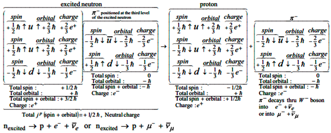
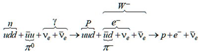
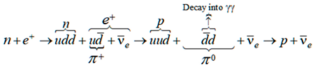
The neutron excited state: While exchanging pions within the nucleous, the neutron absorbs a neutral meason

π^{0}

that changes its inner binding energy configuration by a new generated

π^{-}

meson (see the schema below) that reaches the third orbital level in a momentarily status which creats an excited neutron with a neutral charge and

1 / 2 ℏ

spin. The

π^{-}

meson doesn't radiate while orbiting at the third level and therefore the energy level ~ 80 [Gev] releted to the third level is unnoticeable! The all process of the neutron decaying to a proton is described in the following schemas. Please notice that in addition to the quark's fractional spin and electrical chrage, it has a fractional orbital angular momentum (per energy level) presented in the following schemas.

Neutron absorbing process

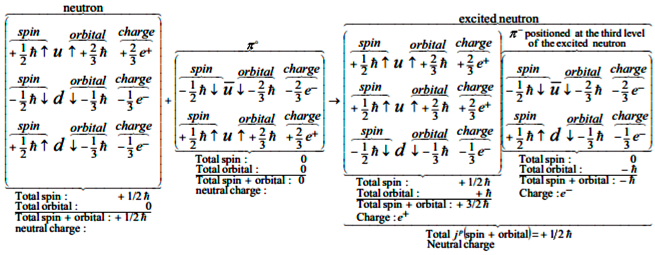
Neutron decaying process

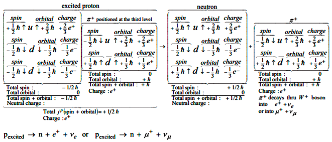
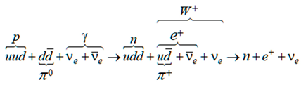
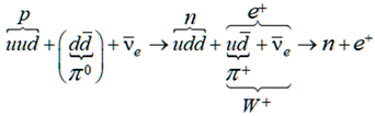
The proton excited state: While exchanging pions within the nucleolus the proton absorbs a neutral meson

π^{0}

that changes its inner binding energy configuration by a new generated

π^{+}

meson (see the schema below) that reaches the third orbital level in a momentarily status that creats an excited proton with a

e^{+}

charge and

1 / 2 ℏ

spin. The

π^{+}

meson doesn't radiate while orbiting at the third level and therefore the energy level ~ 80 [Gev] releted to the third level is unnoticeable. The proton decaying into a neutron in a schema as follows:

Proton absorbing process

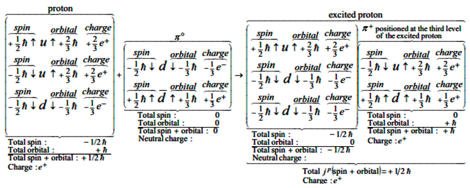
Proton decaying process

a. Beta minus decay:

A neutron, moving free in space (in other words, not in a nucleus) is unstable and decays into a proton, an electron, and an electron antineutrino:

n \to P + e^{-} + \bar{ν}

b. Beta Plus decay :

A proton in a nucleus is converted into a neutron , a positron and a neutrino:

p \to n + e^{+} + ν_{e}

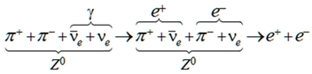
c. The decay of the $Z^{0}$ boson:

$Z^{0}$ boson is a bound state composition of a

π^{+}

and a

π^{-}

mesons and an electron anti-neutrino and an electron neutrino:

Z^{0} \to e^{+} + e^{-}

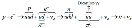
d. The protonsʹ electron capture decay:

The protons can transform into neutrons through the process of electron capture (also known as inverse beta decay:

p + e^{-} \to n + ν_{e}

e. The neutronʹs positron capture (theoretically):

The neutron can transform into proton through the process :

n + e^{+} \to p + {\bar{ν}}_{e}

f. The inverse beta decay:

At this decay process an exchange of a

π^{0}

pion must take place. The

π^{0}

pion is absorbed within the proton and change the inner binding configuration to generate a

π^{+}

pion at the third level which will creat a bound composition with the

{\bar{ν}}_{e}

(anti-neutrino) to form the emitted positron

e^{+}

:

p + {\bar{ν}}_{e} \to n + e^{+}

Conclusions

a. The conclusions from Eq. (85) for the electron wave function of 'Hydrogen like Atom'

R_{n l} (r)

that it is mainly a function of the changing value of the square of the magnetic flux quantum

n Φ_{0}^{2}

and the number of electrons

Z m_{e}

at the relevant level (Please notice that the number of electrons in a neutral atom is equal to the number of protons in the nucleus of the atom presented as the atomic number

Z

).

b. The electron wave function in a 'Hydrogen-like atom' depends on the radius

r

of the atomic level expressed by several Bohr radii, and since the Bohr radius is a function of the square of the magnetic flux quantum , the electron wave function describes the magnitude of the flow pattern of the magnetic flux that surrounds the electrons at the energy levels in the atom.

c. The mass of the electron and other subatomic particles is related to the magnitude of the square of the magnetic flux quantum which makes up the particles. This relationship results in a novel expression of universal constants. The formalism developed in this paper yields the radii of the proton and the neutron from theory.

d. The Gravitational constant is identified based on Newton's law of universal gravitation. The new formula for the Gravitational constant developed in this paper contains elements from the atomic domain (proton's mass and radius) presented by the new proposed Stoney and Planck units, which represent the quantum reality environment; in this way they demonstrate the integration of the quantum and gravity levels.

e. I raise here (as an educated guess) a possibility from obserbing the equations obtained in this article, like for the elementary electric charge in Eq. (16) and Planck's constant in Eq.(19), and especially in the equation for the mass of the electron at Eq. (14), that the product(

α ε_{0}

) that appears in them and in some other equations, describes the size of the electron rest radius

r_{e}

:

r_{e} = α ε_{0} = 6.461213018 \times 1 0^{- 14} m (or double of it!)

f. The proton, the netron and all the baryons consist of two energy levels on which the quarks are orbiting . The third energy level is equivalent to ~ 80 [Gev] ; It plays a major role at decaying process through the weak force while it hosts charged mesons for split seconds which are emitted out through a

W^{-}

boson or

W^{+}

that acquier the level's energy ~ 80 [Gev.

References

Parks, R.D. (1964-12-11). Quantized Magnetic Flux in Superconductors. Science 1964, 146(3650), 14291435. [Google Scholar] [CrossRef] [PubMed]
http://physics.nist.gov/constants.
Beiser, Arthur. Concepts of modern physics. —, 6th ed.; / Arthur Beiser p. cm.Includes index.ISBN 0–07–244848–2 1. Physics. II. Title. QC21.3.B45 20032001044743 CIP.
Barrow, J.D. Natural Units Before Planck. Quarterly Journal of the Royal Astronomical Society 1983QJRAS..24...24B. 1983, 24(24). [Google Scholar]
Wadlinger, R.L.; Hunter, G. Max Planck’s Natural Units. The Physics. 1988. [Google Scholar]
Teacher 26 (528). York University, North York, ONT, Canada M3J 1P. [CrossRef]
Sommerfeld, A. Atombau und Spektrallinien (in German) (2 ed.). Braunschweig, DE: Friedr. Vieweg & Sohn. pp. 241–242, Equation 8. Das Verhältnis v₁/c nennen wir . [The ratio v₁/c we call .] English translation. Methuen & co. 1923. (in German), 2 ed.; 1921; pp. 241–242. [Google Scholar]
Bethke, S. J. Phys. G 2000, 26, R27, [hep-ex/0004021.
Bethke, S.; Dissertori, G.; Salam, G. Quantum Chromodynamics, in K. A. Olive et al. (Particle Data Group). Chin. Phys. C 2014, 38, 090001. [Google Scholar]
The Atomic Nucleus; A.-M. Martensson-Pendrill and M.G.H. Gustavsson Volume 1, Part 6, Chapter 30, pp 477 – 484. In Handbook of Molecular Physics and Quantum Chemistry; ISBN 0 471 62374 1.
Beiser, Arthur.Concepts of modern physics. — 6th ed. / Arthur Beiser p. cm.Includes index.ISBN 0–07–244848–2 1. Physics. II. Title. QC21.3 .B45 20032001044743 CIP page 125.
L.Schiff from his book The Quantum Nechanics, 2^nd ed; McGraw-Hill: New York, 1968; p. 93.
Yukawa, H. On the Interaction of Elementary Particles. Proc. Phys.-Math. Soc. Jpn. 1935, 17(48). [Google Scholar]
Gell-Mann, M. The Eightfold Way: A Theory of Strong Interaction Symmetry. In Synchrotron Laboratory Report CTSL-20; California Institute of Technology, 1961. [Google Scholar] [CrossRef]
The Particle Hunters, by Yuval Ne'eman and Yoram Kirsh, 2nd ed.; Cambridge University Press; Publication date. April 2.

Disclaimer/Publisher’s Note: The statements, opinions and data contained in all publications are solely those of the individual author(s) and contributor(s) and not of MDPI and/or the editor(s). MDPI and/or the editor(s) disclaim responsibility for any injury to people or property resulting from any ideas, methods, instructions or products referred to in the content.

© 2026 by the authors. Licensee MDPI, Basel, Switzerland. This article is an open access article distributed under the terms and conditions of the Creative Commons Attribution (CC BY) license (http://creativecommons.org/licenses/by/4.0/).

Copyright: This open access article is published under a Creative Commons CC BY 4.0 license, which permit the free download, distribution, and reuse, provided that the author and preprint are cited in any reuse.

Particles’ Mass Relationship to the Square of the Magnetic Flux Quantum, and the Quarks at the Three Energy Levels Within the Baryons

Abstract

Keywords:

Subject:

Introduction

Materials and Methods

Results

5. Radius of the proton (hydrogen nucleus).

References

MDPI Initiatives

Important Links

Subscribe