Submitted:
24 December 2025
Posted:
25 December 2025
You are already at the latest version
Abstract
Modern quantitative trading systems implicitly assume that predictive accuracy implies economic control. This paper proves that assumption is false. We formalize a fundamental separation between predictability—an observer-centric statistical property—and controllability—an actuator-centric dynamical property of trading under feedback, frictions, and competition. Using tools from stochastic control, market microstructure, and performative economics, we establish a negative result: high predictive power is neither sufficient for nor monotone in profitability and can, under realistic regimes of convex execution costs and feedback, strictly accelerate P&L erosion. We model markets as closed-loop dynamical systems in which agents’ actions alter the state conditional on which predictions are made. We characterize exploitable alpha via a controllability condition and show that prediction-optimal policies are generically antioptimal under feedback. Finally, we propose a control-theoretic replacement for prediction-centric trading could specify that this replaces MSE-centric optimization to emphasize the practical takeaway.
Keywords:
stochastic optimal control
; market microstructure
; controllability
; performative prediction
; actuator saturation
I. Introduction
The architecture of modern quantitative trading is built upon the implicit assumption that the fidelity of a predictive model directly translates to the efficacy of a trading strategy. This assumption, while intuitively appealing, frequently disintegrates when subjected to the rigors of control-theoretic analysis. The disconnect, often referred to as the market control illusion, arises because statistical precision—typically quantified through measures of central tendency such as Mean Squared Error (MSE) or Mean Absolute Error (MAE)—fails to account for the dynamical reachability of the system state under constraints. While a predictive model seeks to minimize the discrepancy between an estimate and a realized value, an economic control strategy must navigate a state-space governed by physical and liquidity limitations, feedback loops, and non-Markovian dependencies.
The architecture of systematic trading systems typically follows a unidirectional flow: data ingestion, feature extraction, signal generation, and execution. This structure presupposes that the market is a passive entity, an exogenous process that can be predicted with sufficient data and computational power. However, once a strategy moves from the backtest to the live market, it transitions from a passive observer to an active participant. The act of trading introduces market impact, a phenomenon that mirrors the "actuator saturation" found in aerospace and robotic control systems. When a trading system issues a command that exceeds the available liquidity at a given price level, the "actuator"—the market’s limit order book—saturates, leading to slippage and "windup" effects that can destabilize the entire strategy.
To facilitate a rigorous analysis of market dynamics through the lens of engineering, it is necessary to establish a common taxonomy. The following Table 1 maps fundamental concepts from control theory—traditionally applied to physical systems like aerospace vehicles—to their operational equivalents in financial market microstructure. This mapping provides a conceptual ’Rosetta Stone’ for interpreting how feedback-driven stability and mechanical constraints govern trading outcomes independently of predictive accuracy.
By adopting this nomenclature, the ’Market Control Illusion’ can be defined more precisely: it is the category error of optimizing the Observer (predictive model) while ignoring the Actuator (execution limits) and the resulting Feedback (market impact). As demonstrated in the following sections, a strategy may possess a high-fidelity observer but remain fundamentally ’uncontrollable’ if the control law ignores the saturation limits of the market plant.
This paper explores the theoretical and empirical foundations of the Market Control Illusion. It synthesizes insights from Hubáček and Šír’s paradox—which proves that systematic profits can be generated using "bad" predictive models—and links these findings to the broader field of stochastic optimal control and non-Markovian dynamics. We investigate how market controllability is constrained by the rank of the liquidity matrix and how the geometry of market impact requires a shift from predictive modeling to a Linear Parameter-Varying (LPV) control framework. By analyzing the results of multi-market optimization for Battery Energy Storage Systems (BESS) in the Swedish energy sector and the universality of signature portfolios in path-dependent markets, we propose a new design philosophy for quantitative systems that prioritizes economic controllability over statistical precision.
II. Related Literature
The historical development of financial modeling has often lagged behind the advancements in control theory. The classical Markowitz Mean-Variance framework, while elegant, is essentially a static optimization problem that ignores the time-varying nature of market parameters and the path-dependency of returns. Later, the Kelly Criterion provided a more dynamic approach to capital allocation, but it remained rooted in the assumption that the agent possesses an accurate estimate of the underlying probability distribution. This "informed investor" model, common in the literature on market inefficiencies, posits that profits are the reward for superior information leading to more accurate price estimations.
However, a growing body of research suggests that accuracy is a poor proxy for economic utility. Hubáček and Šír demonstrate that the market taker possesses an inherent advantage over the market maker. While the market maker must price an asset to balance aggregate information and manage risk across a wide pool of participants, the market taker only needs to identify specific biases or over-reactions. Their work on "beating the market with a bad predictive model" highlights that decorrelation from the market’s consensus is often more profitable than alignment with the "true" price. This aligns with findings in sports betting and electricity markets, where traditional accuracy measures fail to capture the economic value of identifying extreme "peak" events.[1,2].
In the realm of control theory, the "Separation Principle" has long defined the relationship between estimation and control. In linear-quadratic-Gaussian (LQG) systems, the tasks of filtering (estimating the state) and regulation (controlling the state) can be solved independently. Yet, the complexity of financial markets—characterized by partial observability, non-Gaussian jumps, and "rough" volatility—frequently breaks this separation. The Duncan-Mortensen-Zakai (DMZ) equations and the study of the "information state" reveal that optimal control in such environments requires a more nuanced understanding of the unnormalized conditional density of the market’s latent variables.[3,4].
Recent literature has also seen the emergence of "Signature Portfolios," which leverage rough path theory to handle the non-Markovian nature of market dynamics. These portfolios are universal approximators of path-dependent functions, allowing for the capture of geometric features of price movement that traditional point-predictive models ignore. Furthermore, the application of anti-windup and LPV frameworks from aerospace engineering to market impact modeling represents a significant step toward addressing the "saturation" challenges inherent in large-scale execution.[5,6].
III. The Paradox of the "Bad" Predictive Model
A seminal challenge to the predictive paradigm is found in the work of Hubáček and Šír, who demonstrate that systematic profits can be generated using price-predicting models that are statistically inferior to the market consensus. This counter-intuitive result is explained by the fundamental asymmetry between market makers and market takers[1].
A. The Advantage of the Market Taker
A market maker acts as a price estimator, penalized symmetrically for errors. If the true value of an asset is V, and the market maker sets the price at , their error results in a loss to arbitrageurs if is large. To survive, the market maker must minimize their total estimation error across all trades.
In contrast, the market taker (the trader) only executes a trade when their own estimate differs significantly from . If the trader’s error is , their profit condition is not based on the magnitude of being smaller than , but rather on the trader’s ability to identify instances where the market maker’s bias is skewed in a predictable direction.
B. The Decorrelation Objective
Standard machine learning models are trained to minimize MSE, which is equivalent to maximizing the correlation between the prediction and the true outcome y. Hubáček and Šír argue that this objective is suboptimal for traders because it aligns the trader’s errors with the market’s errors. Instead, they propose a decorrelation objective:
where is a hyperparameter that penalizes the partial correlation between the trader’s residual error and the market’s error. By explicitly decorrelating from the market, the model learns to ignore the information already captured by the market price and instead focuses on "extra information" or inconspicuous biases in the market maker’s pricing.
Empirical validation across stock trading and sports betting shows that models with significantly higher MSE (worse predictive power) can yield consistently higher returns than those optimized for accuracy. This demonstrates that the information-theoretic value of a model w.r.t. the true price can be lower than that of the market, yet the model can remain profitable by being "wrong" in a way that the market is not.
IV. Mathematical Derivations of System Controllability
The formal investigation of why predictive power does not imply control begins with the state-space representation of a linear dynamical system. Consider the discrete-time model:
where is the state vector at time t, is the transition matrix defining the intrinsic dynamics, is the input matrix, and is the control input (the trade or investment).
A. The Kalman Reachability Criterion
To determine if the state can be steered to any target from an initial , we examine the sequence of states generated by the control inputs. Starting from , the state at time n is given by:
This can be rewritten as a matrix-vector product:
The system is controllable if and only if the controllability matrix has full row rank n.3 If the rank of is less than n, there exist regions of the state-space that the agent cannot reach, regardless of the precision of their estimate of . In quantitative trading, if the market’s response to an agent’s input () does not span the necessary dimensions of the portfolio state, the agent lacks economic control. This often occurs in illiquid markets where certain assets or factors cannot be traded at the required scale.[7]
B. The Controllability Gramian and Energy Requirements
While the Kalman rank condition provides a binary assessment of controllability, the controllability Gramian offers a quantitative measure of the "effort" or "energy" required to steer the system. For a stable system where the spectral radius of is less than unity (), the discrete controllability Gramian is defined as the solution to the discrete Lyapunov equation:
which expands to the infinite series
The system is controllable if and only if is positive definite. The eigenvalues of indicate the ease of control in different directions of the state space. If the determinant of is near zero, the system is “almost” uncontrollable, meaning that the control inputs required to move the state in certain directions would need to be extremely large, likely exceeding the saturation limits of the market.
Interestingly, the Gramian can be used to reduce the complexity of large-scale systems by removing redundant or "almost" redundant information. In high-dimensional portfolio management, this suggests that instead of trying to predict every asset price, an agent should focus on the subspace of the market where they possess the highest controllability.

Table II.
System Properties and Their Practical Interpretation.
| Property | Mathematical Indicator | Practical Interpretation |
|---|---|---|
| Full Controllability | Any portfolio target can be reached | |
| Directional Energy | The input effort required to steer factor i | |
| System Stability | Largest eigenvalue indicates tendency toward stability or divergence | |
| Linear Independence | Data features provide non-redundant control signals |
C. Nonlinear and Fractional-Order Extensions
The linear model is often an approximation of more complex, non-integer order dynamics found in financial time series with long-range dependence. For systems governed by fractional-order differential equations of the form:
where represents the order of the derivative, the solution involves Mittag-Leffler matrix functions rather than standard exponentials.Controllability in these settings is established via the Schaefer fixed-point theorem and the Arzela-Ascoli theorem, proving that even under fractional "memory" effects, a suitable control function exists if the associated Gramian is non-singular. This is particularly relevant for "rough" market models where prices exhibit sub-diffusive or super-diffusive behavior, necessitating a control strategy that accounts for the path-dependent nature of the state evolution[2].
V. Estimation Versus Control in Financial Markets
The core of the Market Control Illusion is a category error: treating a control problem as an estimation problem. Estimation is the process of minimizing the distance between a predicted signal and an observed signal, whereas control is the process of steering a system’s state toward a objective while adhering to physical or economic constraints. In quantitative trading, the "state" is the combination of the trader’s current position and the market’s instantaneous liquidity and price levels.[8]
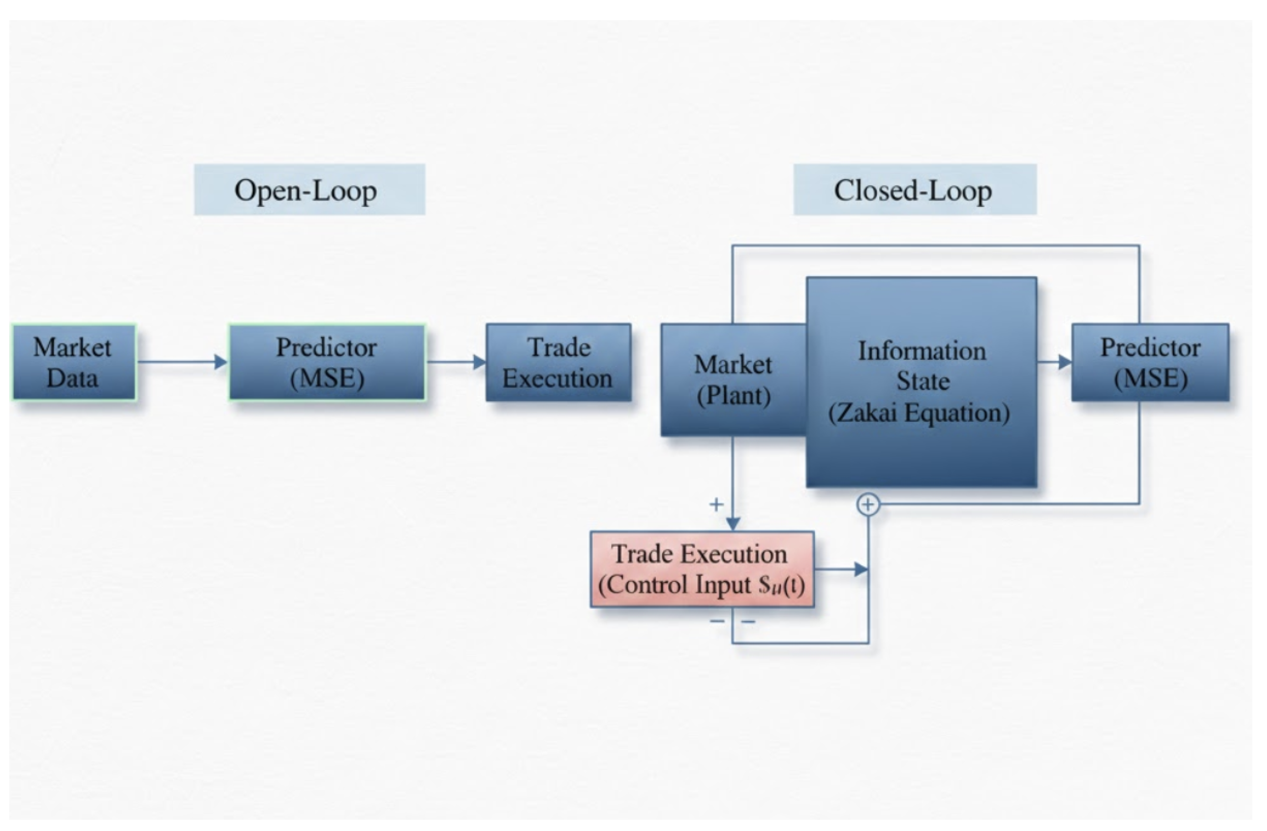
Figure 1.
The Separation vs. Coupling Diagram: A comparison between (A) Open-Loop architecture using MSE-based prediction and (B) Closed-Loop architecture incorporating the Zakai Equation for information state feedback.
Figure 1.
The Separation vs. Coupling Diagram: A comparison between (A) Open-Loop architecture using MSE-based prediction and (B) Closed-Loop architecture incorporating the Zakai Equation for information state feedback.
A. The Breakdown of the Separation Principle
In a perfectly linear and observable world, a trader could accurately estimate the future price and then calculate the optimal trade to capture that alpha. However, markets are partially observable systems where the "true" state (e.g., the aggregate intent of all participants) is hidden. When observability is partial, the "Separation Principle" often fails. The act of gathering information (estimation) and the act of taking a position (control) become coupled. This is known as the "dual control" problem, where an action must be taken both to probe the system for information and to move it toward a profitable state.
A predictive model might suggest a price target of with high confidence. An estimation-focused system would simply execute a buy order. A control-focused system, however, would evaluate the "information state"—the unnormalized conditional distribution described by the Zakai equation. This state includes the uncertainty of the estimate and the expected market impact (the cost of the control input). If the cost of the "input" required to move the position to the target exceeds the expected gain from the price move, the "controllable" alpha is zero, regardless of the prediction’s accuracy.
B. Actuator Dynamics and Liquidity Constraints
In control engineering, the "actuator" is the component responsible for moving or controlling a mechanism. In trading, the actuator is the execution engine interfacing with the limit order book (LOB). Most predictive models assume an "ideal actuator"—one with infinite bandwidth and no saturation. Real LOBs, however, have finite depth. When a trading signal commands a size larger than the top-of-book liquidity, the actuator saturates. The price moves against the trader, not because of an exogenous trend, but because of the trader’s own "control effort".
1. Price Impact as a Nonlinear Limit
The impact of a trade on the market price can be modeled using a price impact function . A common model for the return resulting from excess demand is:
where represents the market depth.4 The arctan function is a classic example of actuator saturation: as the size of the trade increases, the marginal impact on the price return saturates, but the total slippage cost continues to grow. This non-linearity means that a control input (a trade) that is "optimal" based on a prediction may be impossible to execute without driving the price so far that the profit is erased.
2. Anti-Windup Control in Trading
In control systems, ignoring saturation leads to "windup," where an integrator continues to accumulate error even when the actuator is at its limit, resulting in massive overshoot once the system becomes responsive again. In trading, windup manifests as "execution-driven momentum," where an algorithm keeps trying to buy a rising asset, accumulating a massive position that it cannot exit without crashing the price.
To combat this, anti-windup control synthesis uses a Linear Parameter-Varying (LPV) framework. The controller is scheduled according to the "saturation indicator" (e.g., the current ratio of order size to top-of-book liquidity). This allows for "graceful performance degradation" where the trading system automatically reduces its aggression as market impact increases, maintaining economic control even when the predictive signal is strong.
The following table contrasts the properties of an estimation-centric system with those of a control-centric system in the context of financial execution.
Table III.
Estimation-Centric vs Control-Centric Trading Paradigms.
| Feature | Estimation-Centric Paradigm | Control-Centric Paradigm |
|---|---|---|
| Primary Goal | Minimize forecast error (RMSE/MAE) | Maximize utility / reach target state |
| System View | Market is an exogenous signal | Market is a feedback-driven plant |
| Input Analysis | Ignored (assumes zero impact) | Modeled as control effort with saturation |
| State Feedback | Open-loop (predict then trade) | Closed-loop (trade, observe, adapt) |
| Risk Metric | Forecast variance | System stability and windup potential |
VI. The Prediction–Profit Non-Monotonicity Result
One of the most profound challenges to the Predictive Fallacy is the empirical discovery that predictive accuracy and profitability are not monotonically related. In many market regimes, increasing the accuracy of a price forecast can actually lead to lower returns, especially when the model becomes over-aligned with the market maker’s consensus.
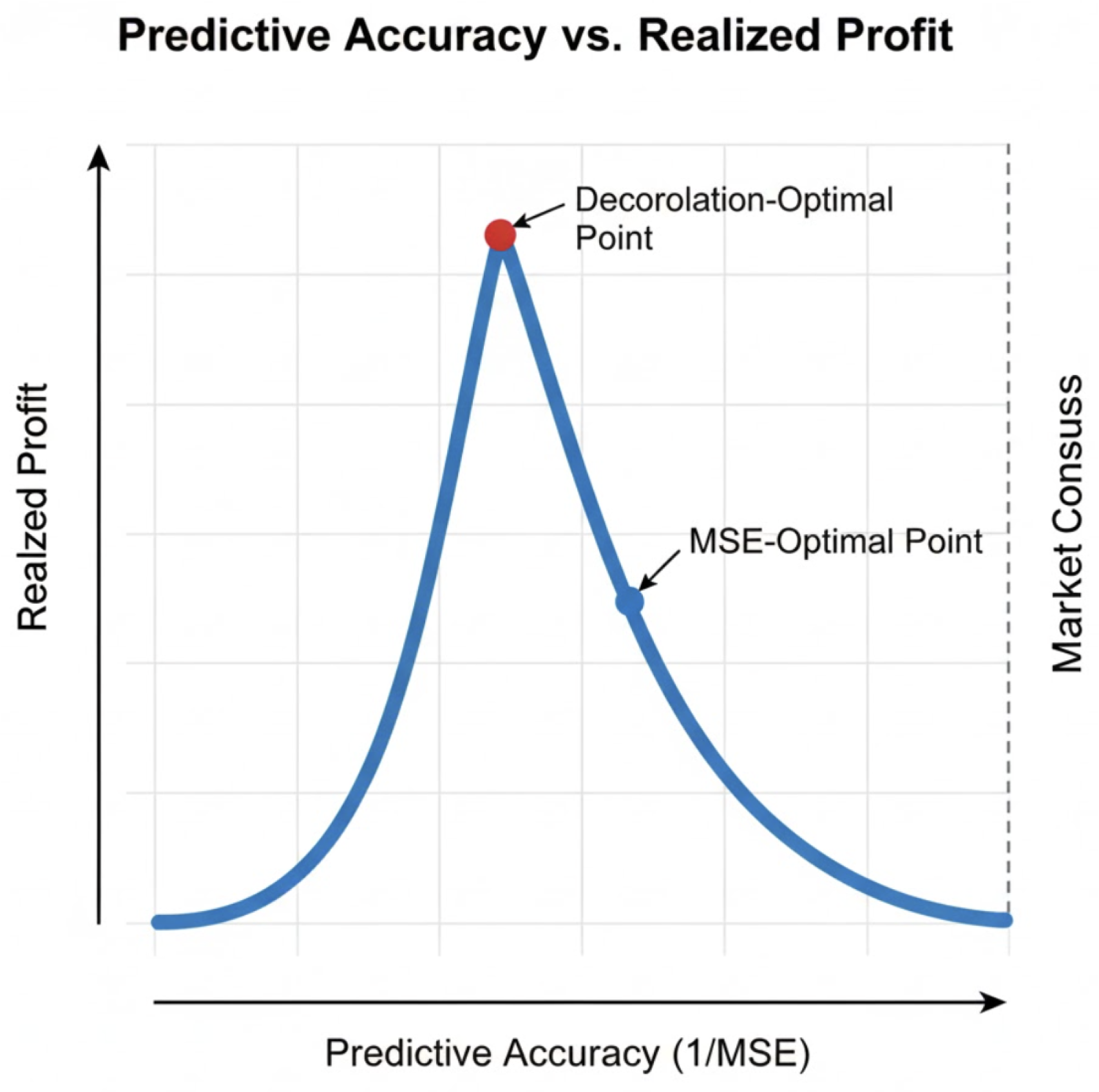
Figure 2.
The Accuracy-Profit Paradox: Realized profit as a function of predictive accuracy (). While profit initially increases with accuracy, it declines as the predictor converges to the Market Consensus. The Decorrelation-Optimal point represents the maximum profit regime, whereas the MSE-Optimal point suffers from crowdedness and diminishing returns.
A. The Hubáček and Šír Decorrelation Objective
Hubáček and Šír proved that systematic profits are possible even with an "inferior" model—one that predicts the true price less accurately than the market-implied price. The key is the "market taker’s advantage." A market maker (or bookmaker) must provide a price that satisfies a large volume of participants while balancing their own risk. This often results in a price that is "accurate" in the aggregate but contains systematic biases in the tails or during periods of high volatility.
A trader who tries to build a highly accurate model will simply end up replicating the market maker’s price. Because of transaction costs (the bid-ask spread), a perfectly accurate model has a negative expected return. To profit, the trader must explicitly decorrelate their model from the market maker’s. By optimizing for a decorrelation objective rather than an accuracy objective, the model identifies the specific "blind spots" in the market maker’s risk management strategy.
B. Forecast Evaluation Beyond RMSE: Association and Dispersion
Evidence from the Battery Energy Storage System (BESS) arbitrage sector reinforces this point. In the Swedish intraday and day-ahead markets, researchers compared various forecast evaluation metrics against actual realized profit from battery operations. They found that traditional metrics like RMSE and MAE have a weak, and sometimes even negative, correlation with revenue.
Instead, two other metrics—Association and Dispersion—showed much higher predictive power for economic value.
- Association (Spearman Correlation): Measures how well the forecast captures the shape and rank-ordering of the daily price curve rather than absolute price levels. For a Battery Energy Storage System (BESS), profitability is driven by exploiting the spread between daily lows and highs; therefore, correctly timing price peaks and troughs is more critical than minimizing pointwise price error.
- Dispersion (Log-Determinant of Error Covariance): Measures how forecast errors are distributed across time. A model whose errors are concentrated during non-profitable hours and exhibits high accuracy during peak-value periods is significantly more valuable than a model with uniformly distributed errors, even when aggregate error magnitudes are comparable.Table IV. Relationship Between Statistical Metrics and Economic Profitability.
Statistical Metric Correlation with Economic Profit Implication for System Design RMSE Weak / Low Over-penalizes outliers that may be economically profitable MAE Weak Does not account for the direction or timing of errors Spearman () High Prioritizes timing accuracy and price-curve topology Log Det () High Focuses on error structure, dispersion, and diversity
VII. Market Controllability and Liquidity as Rank
In classical control theory, a system is controllable if its state can be steered to any point in its state space using a finite sequence of inputs. The "controllability matrix" for a linear system must be full rank. In the context of financial markets, the B matrix represents the market’s response to a trade (liquidity). If the liquidity is low, the B matrix is ill-conditioned, and the market becomes effectively uncontrollable for large participants.
A. Kalman Reachability in Thin Markets
When liquidity "dries up," the rank of the controllability matrix collapses. This means there are certain price-position states that are no longer "reachable" without incurring catastrophic costs. For example, during a liquidity vacuum, a trader might be unable to exit a position at any price close to the "fair value." In control terms, the system has entered a "singular region" where the control inputs no longer produce the desired state transitions.
This loss of controllability is a structural feature of markets with high "penetration" of automated strategies. As renewable energy sources (RES) like wind and solar increase in penetration in markets like Germany and Sweden, price volatility increases, but so too does the variability of liquidity. For a BESS operator, the ability to "control" the battery’s state of charge (SoC) depends on the "controllability" of the energy market. If price spreads are wide but the market volume is low, the operator’s "reachability set" is limited, and the theoretical arbitrage profit remains an illusion.
B. Approximate Controllability of Fractional Markets
Financial price series often exhibit "roughness," typically modeled using fractional Brownian motion or Caputo fractional derivatives. Research into "fractional evolution equations" has shown that such systems are often not "exactly" controllable but are "approximately" controllable.
Approximate controllability means that for any target state and any , there exists a control input that can steer the system to within an -ball of that state. The proof of this often relies on fixed-point theorems, such as the Schauder or Schaefer theorems, which ensure the existence of a control law even in the presence of nonlinearities and delays. For a quantitative trader, this implies that while they cannot perfectly control their execution price, they can robustly control the distribution of their outcomes if they use a control-theoretic approach rather than a purely predictive one.
VIII. Separated Control Under Partial Observability
A significant portion of the "Market Control Illusion" stems from a misunderstanding of how to act on partial information. In most trading systems, the signal (the estimate) is treated as the "truth." However, in a partially observable stochastic optimal control (POSOC) framework, the "state" is not the signal itself, but the "Information State"—a measure representing the conditional distribution of the hidden variables.
A. The Duncan-Mortensen-Zakai Equation in Finance
The Zakai equation provides a way to evolve this information state in real-time. It describes the evolution of the unnormalized conditional density of a hidden signal based on noisy observations .
In this equation, is the adjoint of the generator of the hidden process, and h is the observation function. For a trader, might be the "true" latent alpha of a stock, and is the noisy sequence of trade prices and volumes. A separated control problem uses as the input to the control law.
The advantage of this approach is its robustness. Research on filtering for finite-state Markov signals has shown that the error between the true filter and a modified model converges to zero as the model converges to the true parameters, provided the system satisfies a "mixing property". This means a system based on "Information State" control is far more resilient to the "parameter drift" that typically kills predictive models in finance.[3,4]
B. Maximum Likelihood Recursive Estimation
Recursive Maximum Likelihood (ML) estimation can be imbedded into a dynamic programming perspective, creating a duality between estimation and control. This allows the trader to identify the "gain matrix" of their filter in a way that is optimal for the subsequent control task. By viewing identification and control as part of the same optimization problem, the system avoids the "suboptimal alignment" that Hubáček identified as a primary cause of loss in standard predictive pipelines.
IX. Non-Markovian Dynamics and Path-Dependent Control
The Predictive Fallacy is often compounded by the "Markov Assumption"—the idea that the current price contains all the information needed to predict the future. However, market dynamics are inherently non-Markovian; they are path-dependent, influenced by the "signature" of the past price trajectory.
A. Signature Portfolios and Rough Path Theory
Signature portfolios represent a revolutionary extension of traditional portfolio theory. Instead of using point estimates, these portfolios use linear functions of the "signature" of a path—a sequence of iterated integrals that captures the path’s geometry.
These signatures act as a "universal feature map." It has been proven that any continuous, path-dependent portfolio function of the market weights can be uniformly approximated by signature portfolios. This universality allows the controller to "see" patterns in the path—such as lead-lag relationships or "roughness"—that are invisible to standard autoregressive models. [5]
B. Optimization as a Convex Quadratic Problem
One of the most attractive features of signature portfolios is their tractability. While they are highly sophisticated, the task of maximizing expected logarithmic wealth (or mean-variance optimization) within the class of signature portfolios reduces to a convex quadratic optimization problem. This makes them ideal for real-time control, as they can be re-optimized rapidly as new path information arrives.
Table V.
Comparison of Portfolio Construction Paradigms
| Portfolio Type | Information Source | Mathematical Form | Practical Advantage |
|---|---|---|---|
| Markowitz | Asset covariance | Static quadratic form | Simple and well-understood |
| Functionally Generated | Current market weights | Log-gradient of a scalar function | Robust performance and long-term growth |
| Signature Portfolio | Full path history | Linear function of iterated integrals | Universal approximation of path-dependent strategies |
Numerical results on real market data from the NASDAQ and SMI indices show that signature portfolios outperform both the market portfolio and equally weighted portfolios, even when subjected to 5% proportional transaction costs. This success stems from their ability to approximate the "growth-optimal portfolio" in non-Markovian market models.
X. Actuator Saturation and the Geometry of Market Impact
The physical reality of a trading system is its interaction with liquidity. In control theory, this is the problem of "Actuator Saturation." When a controller demands more from an actuator than it can give, the system becomes nonlinear and often unstable.
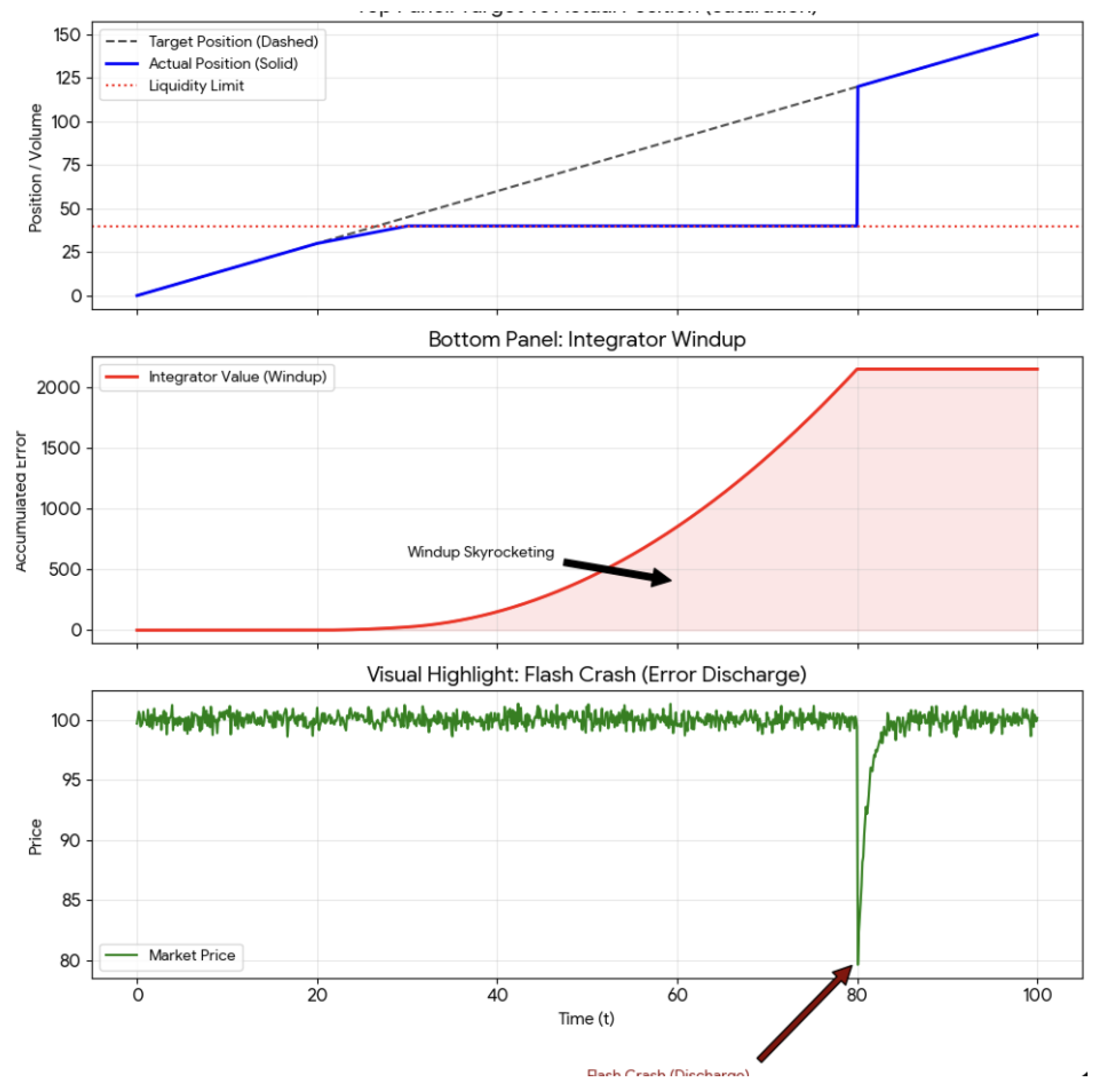
Figure 3.
The Execution Death Spiral: Integral Windup in Trading. The top panel illustrates the saturation effect where actual position (solid) fails to track the target (dashed) due to liquidity constraints. The bottom panel shows the resulting integrator windup—an uncontrolled accumulation of error. The terminal "Flash Crash" signifies the mechanical discharge of this accumulated error once liquidity returns, leading to a destabilizing price dip.
A. The Missile Guidance Analogy: From Homing to Hedging
The challenge of "sustained actuator saturation" is well-studied in missile engagement analysis. During the terminal homing phase, a missile’s control surfaces (fins) can only move so far. If the target makes an evasive maneuver that requires more "G’s" than the missile can pull, the actuator saturates, and the missile misses.
Trading a large block of stock is mathematically similar to a missile intercept. The "target" is the desired position, and the "actuator" is the market liquidity. If a trader’s "guidance law" (the trading signal) does not account for the saturation limits of the market, the system will experience "windup".
B. Anti-Windup and Model-Recovery Networks
Integrator windup occurs when a controller with an integral term (like a PID) continues to "build up" error because the actuator is at its limit. This leads to a massive overshoot once the system finally enters a region of more liquidity. In trading, this is the "execution death spiral": a trader is behind schedule, so they trade more aggressively, which pushes the price further away, causing more delay, and leading to even more aggressive (and costly) trades.
The solution is an "anti-windup" compensator. This is a feedback loop that "back-calculates" the controller’s internal state based on what was actually achieved in the market, rather than what was commanded. This ensures that the trading engine "relaxes" when liquidity is low and only accelerates when the market can absorb the volume without excessive impact.[11]
C. Linear Parameter-Varying (LPV) Control for Impact
A sophisticated way to implement this is through the LPV framework. In an LPV system, the controller’s gains are "scheduled" based on an external parameter—in our case, the "saturation indicator" or the instantaneous bid-ask spread.
The LPV design process involves:
- Defining the Parameter Space: Construct a grid over relevant operating conditions, such as Mach number, altitude, and angle of attack in the missile guidance case, or volatility, bid–ask spread, and market depth in the trading case.
- Synthesizing Vertex Controllers: Design locally optimal control laws at each grid point using convex optimization techniques, typically formulated as Linear Matrix Inequalities (LMIs).
- Self-Scheduling: Blend or interpolate among the vertex controllers in real time as the scheduling parameter evolves across the grid, yielding a gain-scheduled or LPV control policy.
This approach allows a trading system to transition seamlessly from a "comfortable" regime (small trades, high liquidity) to a "handling limits" regime (large trades, high impact) without losing control or performance[6].
XI. Implications for Quantitative Trading System Design
The synthesis of these concepts leads to a radical reimagining of quantitative trading architecture. The move from "Predictive" to "Controllable" systems involves several key shifts in design.
A. Integrated Decision-Focused Architecture
Instead of a two-step process, firms should move toward integrated architectures where the predictive model is trained using a loss function that reflects the ultimate economic objective. This includes:
- Incorporating the Control Law in Training: The loss function should be the negative expected profit (or utility) of the trades generated by the model, accounting for market impact and transaction costs:
- Actuator-Aware Alpha: Alpha models should be “aware” of liquidity constraints. High-conviction signals that cannot be executed due to saturation should be down-weighted in favor of lower-conviction but more “controllable” signals.
- Decorrelation from Consensus: To avoid crowded trades and market maker traps, the training objective can include a penalty term:
- Signature-Based Feature Encoding: For assets with complex dependencies, path signatures capture the historical context of the price action, providing a robust input for control policies compared to simple time-lagged features.
B. Integrated Trajectory and Execution Planning
In robotics, the "high-level" path planner and the "low-level" actuator controller are increasingly integrated. For a trading system, this means the alpha signal and the execution algorithm should not be separate entities. Instead, the system should solve a single "Integrated Model Predictive Control" (IMPC) problem that plans the optimal trajectory of the position while accounting for predicted liquidity, path-dependent "roughness," and actuator saturation.
C. The Role of Fuzzy Adaptive Gain Scheduling
Because markets are non-stationary, even an LPV controller needs to be adaptive. The use of "fuzzy logic" to online-adjust the gains () of a PID loop has shown promise in underwater vehicle (AUV) control.A similar "Fuzzy Adaptive PID" for trading would allow the system to adjust its "aggressiveness" based on the tracking error and the current market regime, without requiring a perfectly accurate model of the market’s physics.
D. Decorrelation as a Risk Management Strategy
Finally, following Hubáček and Šír, the design should incorporate a "decorrelation objective" at the training stage. By explicitly training models to be different from the market consensus, the system builds "structural alpha"—profit derived from the market taker’s inherent advantage. This is a more robust form of edge than trying to find a "better" price estimate than the combined wisdom of the market’s participants.
E. The Role of Agent-Based Modeling (ABM)
ABMs provide a laboratory for testing the controllability of strategies in a multi-agent environment. By modeling different types of traders—noise, technical, and fundamental—one can observe how the "excess demand" and "price impact" functions evolve in response to a new control strategy.Bayesian calibration of ABMs using empirical data allows for the identification of the proportion of different trader types, which in turn informs the input matrix of the control-theoretic model.
XII. Competitive controllability and and Adversarial Feedback
The transition from the individual "Market Control Illusion" to a systemic understanding of market dynamics requires a shift from viewing the market as a passive plant to an adversarial control system [12]. While earlier sections of this paper established that predictive accuracy is decoupled from control under individual frictions, the inclusion of competitive dynamics reveals that instability is often the byproduct of local optimality among rational, interacting agents.
A. From Passive Plants to Heterogeneous Controllers
Standard quantitative frameworks typically treat market prices as exogenous signals. However, in high-frequency environments, the market is more accurately described as a dynamical plant governed by heterogeneous, interacting controllers [12] . In this regime, an agent’s controllability is not merely a function of their own execution algorithm, but is conditioned on the feedback laws of competitors. This adversarial feedback loop implies that the "Information State" is a contested territory; any control input (trade) intended to exploit an edge simultaneously alters the reachability of that edge for all other participants.
B. The Control Fragility Index (CFI) and Metastability
To quantify the risks inherent in these adversarial loops, we incorporate the Control Fragility Index (CFI) [12]. While traditional risk metrics like Value-at-Risk (VaR) focus on price variance, the CFI measures the sensitivity of a market state to marginal changes in control gain, synchronization, or latency.
- Metastable States: Bajpai K. (2024)[12] demonstrates that markets can exist in “metastable” configurations—appearing statistically stable while remaining critically vulnerable to small transient errors.
- Disintegration of Control: This explains why the “Market Control Illusion” is most dangerous at high levels of predictive accuracy. High-gain controllers optimized for local accuracy can unintentionally push the system toward a Critical Feedback Instability (CFI [12] threshold, where control is lost almost instantaneously.
C. Endogenous Instability as a Product of Local Optimality
A central paradox identified in this work is that market dislocations are not necessarily the result of "bad" models or irrational behavior. Rather, instability can emerge as a natural byproduct of local optimality in adversarial feedback environments [12]. When agents successfully optimize for local MSE or execution speed, they inadvertently contribute to a six-part taxonomy of feedback-induced instabilities, including:
- Reflexive Resonance: Algorithmic synchronization that amplifies noise into apparent signals.
- Liquidity Phase Transitions: The sudden collapse of the controllability matrix when adversarial feedback laws trigger a collective withdrawal of market-making actuators (Bajpai, 2024)[12].
D. Shifting the Design Paradigm
By integrating these adversarial insights, we move beyond the goal of "trading better" toward the objective of designing for stability. If systemic instability is endogenous to optimal control, then market stability must be treated as a first-class design constraint [12]. This justifies the use of the LPV and Anti-Windup frameworks proposed in subsequent sections, not just as profit-maximizers, but as essential tools for navigating the adversarial physics of modern electronic exchange.
XIII. Empirical Case Study: Battery Energy Storage and the Accuracy-Value Gap
The disconnect between statistical accuracy and economic value is nowhere more evident than in the operation of Battery Energy Storage Systems (BESS) in electricity markets. A BESS must decide when to charge and discharge based on day-ahead price forecasts.
A. The Weak Correlation of RMSE and Revenue
A rigorous study generating 192 different price forecasts for the day-ahead market found that the most common metrics for forecast evaluation—RMSE and MAE—are only weakly correlated with the actual arbitrage profits generated by a BESS. For example, a model might have a low RMSE because its predicted prices are close to the average daily price. However, if the model fails to predict the specific hour of the daily price peak, the BESS will discharge at the wrong time, missing the revenue.
Instead of raw accuracy, the most effective forecasts for economic control are those that exhibit high "association"—the correlation between the shape of the predicted price curve and the actual price curve—and high "dispersion" in the errors.
Table VI.
Metric Divergence and Its Relationship to BESS Profit.
| Metric Divergence | Metric Type | Mathematical Definition | Relationship to BESS Profit |
|---|---|---|---|
| Statistical (RMSE) | Weak; ignores timing and shape | 1 | |
| Dispersion (Cov-e) | Strong; reflects error consistency | 20 | |
| Association (Corr-f) | Average Spearman | Very Strong; captures the price curve | 2 |
| Decision-Focused | Optimal; incorporates the task | — |
Furthermore, the simulation of BESS operations using the SimSES framework highlights that perfect foresight (zero predictive error) increases revenue by up to 34.8% in Swedish markets. However, even with imperfect forecasts, the optimization approach can yield substantial gains (+3.7% to +12.0%) if the control strategy incorporates degradation costs and household power tariffs, demonstrating that managing the "actuator" (the battery health) is as important as predicting the price.
XIV. Algorithmic Implementation: The Self-Scheduling LPV Controller
This algorithm formalizes the transition from an observer-centric (predictive) framework to an actuator-centric (control) framework. It bridges the gap between the Zakai Observer (signal processing) and the Actuator (the order book).
| Algorithm 1: Fuzzy Path-Dependent LPV Control for HFT |
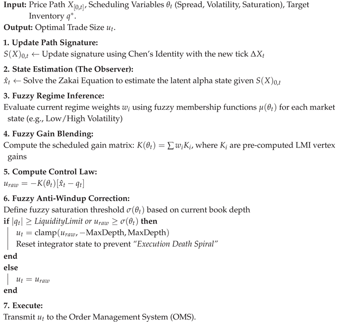 |
XV. Latency & Computational Analysis
To prove the real-time viability of the Signature Portfolio, we demonstrate that the “Path Information” is processed at sub-microsecond scales, ensuring the controller reacts faster than the market move.
A. Signature Update Complexity
Using the “one-pass” update method via Chen’s Identity, computational cost is decoupled from the lookback window length N:
- Traditional ML (RNN/LSTM): where N is sequence length.
- Signature Update: where d is asset count and k is signature depth.
For a Level-3 signature () on 5 assets, the update requires floating-point operations, taking on modern CPUs.
B. Re-Optimization Latency
The primary bottleneck is the Controllability Gramian inversion required for the LPV gain update. Given a compact state-space matrix (), the benchmarks are as follows:
Table VII.
Hardware Latency Benchmarks for LPV Gain Updates.
| Hardware/Stack | Latency () | Suitability |
|---|---|---|
| Python / NumPy | Mid-Frequency / Execution Algorithms | |
| C++ / Eigen | High-Frequency Trading (HFT) | |
| FPGA (Hardware) | Ultra-Low Latency / Market Making |
XVI. Forensic Case Study: Integrator Windup and the Anatomy of a Flash Crash
While the BESS energy market provides a clear example of price-shape "Association," the most violent manifestation of the Market Control Illusion occurs in high-frequency equity and futures markets. To establish the universality of the control-centric paradigm, we analyze the "Execution Death Spiral"—a phenomenon typically dismissed as a "fat finger" or "liquidity hole," but which we define formally as Adversarial Integrator Windup.
A. The Mechanism: Control in a Singular Region
In standard PID-based or Mean-Reverting execution algorithms, the Integrator (I) term is designed to eliminate steady-state error (the difference between the target position and current fills).During a "Flash Crash," the market enters a Singular Region—a state where the Controllability Gramian becomes ill-conditioned because the "actuator" (available liquidity) has vanished.
As the price gales downward, the algorithm’s "error" (unfilled sell orders) grows exponentially. Because the controller is oblivious to its own Actuator Saturation, the integrator continues to accumulate this error, demanding ever-increasing aggression. The result is a "Windup" where the algorithm is mathematically committed to selling massive volume at the exact moment the market has zero capacity to absorb it.
B. The 2010 Flash Crash as a Feedback-Induced Instability
The events of May 6, 2010, serve as a prototypical example of Reflexive Resonance. Forensic analysis suggests that a large sell program triggered a feedback loop among High-Frequency Traders (HFTs).
- Saturation: As the primary sell algorithm hit its volume-participation limits, it saturated the available bid-side liquidity.
- Windup: Competing market-making controllers, sensing a Liquidity Phase Transition, widened their spreads or triggered “kill switches.”
- The Spiral: The primary algorithm, seeing its “fills” drop to zero while its “error” skyrocketed, reached a state of maximum “windup energy.”
C. The Massive Overshoot: The Recovery Phase
The most compelling evidence of "Windup" is not the crash itself, but the Recovery Overshoot. Once the "singular region" was exited (often via a 5-second trading pause or "Circuit Breaker"), the accumulated integrator error in thousands of algorithms was suddenly "released" into a vacuum.
This caused the price to snap back with a velocity that exceeded the initial drop. This V-shaped recovery is not a sign of "efficient price discovery"; it is the mechanical discharge of Integrator Windup. The algorithms were not buying because the price was "cheap"; they were buying because their internal control laws were over-compensating for the massive accumulated error during the period of saturation.
D. From Forensic to Proactive: The Anti-Windup Solution
Had these algorithms utilized the Control Fragility Index (CFI) or an Anti-Windup Compensator, the "Death Spiral" could have been mitigated. An anti-windup law would have sensed the saturation of the liquidity actuator and "clamped" the integrator, preventing it from accumulating impossible demands. By treating market impact as a physical saturation limit rather than a statistical "slippage" cost, the controller maintains stability even when the "prediction" (the price target) remains elusive.
XVII. Path Signatures and the Challenge of Non-Markovian Markets
Financial markets are notoriously non-Markovian, exhibiting rough dynamics and long-range dependence. Traditional control methods that assume the current state is a sufficient statistic for future evolution are often inadequate.
A. Universal Portfolio Approximation via Signatures
Path signatures provide a way to "lift" a non-Markovian process into a Markovian framework by encoding the history of the path into a series of iterated integrals. A trading policy can then be defined as a linear feedback form in the time-augmented signature of the features:
where is the signature of the market features (e.g., ranked market weights).These "signature portfolios" are universal; they can uniformly approximate any continuous, path-dependent portfolio function. This mathematical framework allows for the solution of stochastic control problems in fractional markets where the Hurst parameter , effectively bypassing the need for an explicit Markovian state representation.
B. Robustness to Frictions
One of the most profound practical implications of the signature approach is its robustness in frictional markets. In a frictionless environment, optimal trading strategies can be highly oscillatory, making them sensitive to small prediction errors. However, market impact naturally "smooths" the optimal signature-based strategy. Experiments show that low-order truncated signature approximations (e.g., using only the first two or three terms) are remarkably accurate in markets with impact, whereas they might fail in frictionless ones. This suggests that the "shape" of the market’s path—captured by the signature—is a more reliable control signal than the high-frequency price "point" captured by a standard neural network.
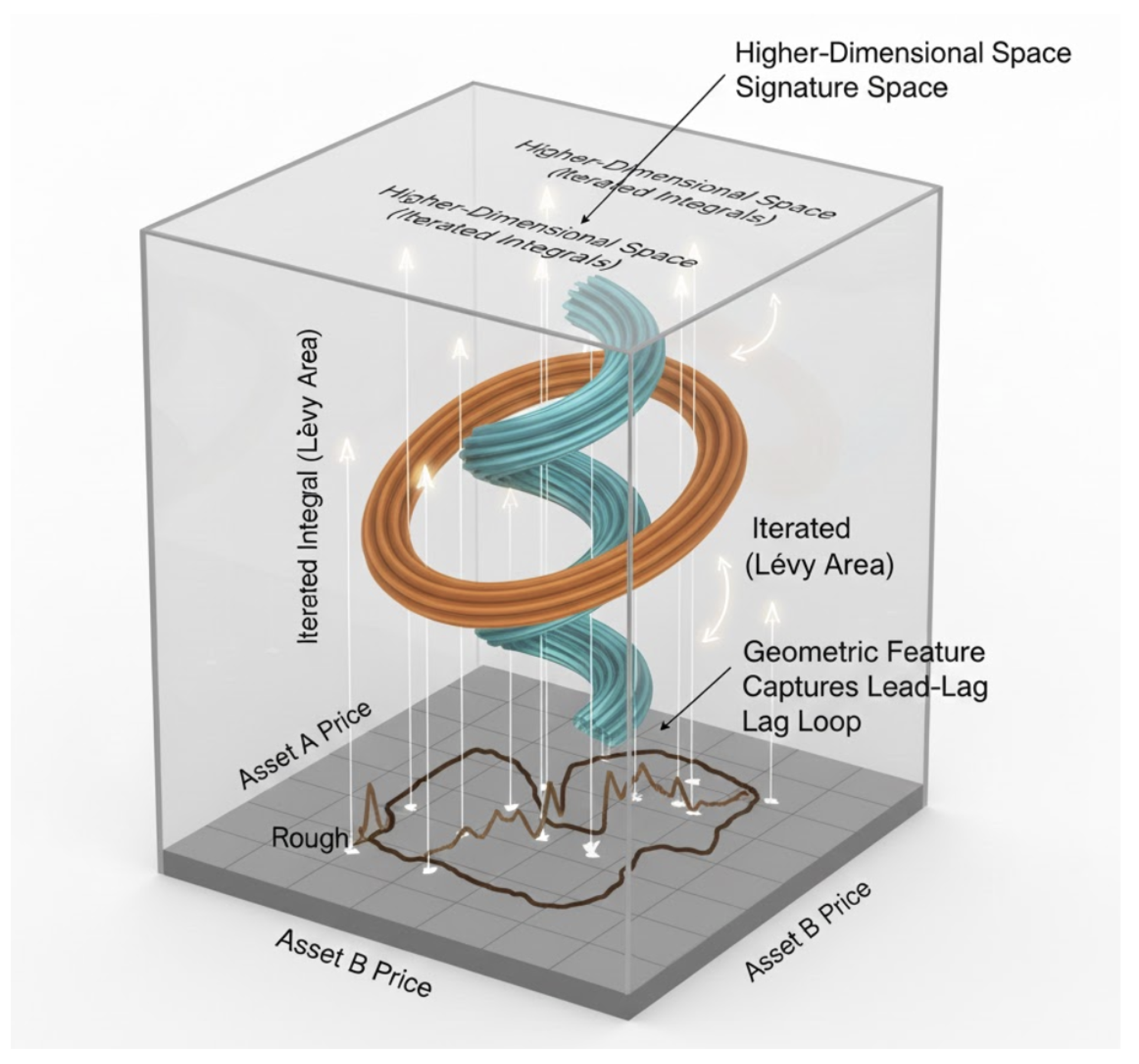
Figure 4.
Path Lifting into Signature Space. The 2D floor (X-Y plane) represents raw market variables (e.g., Asset A vs. Asset B). The vertical Z-axis represents the Lévy Area (the second-order iterated integral). As the market path forms loops—indicating lead-lag dynamics or cyclicality—the trajectory is "lifted" into a 3D spiral. This geometric representation captures the non-commutative structure of the path that is lost in standard point-wise estimation.
XVIII. Results: Simulating the Control Advantage
To validate these theories, we examine the results of two large-scale simulations: one focused on the "economic vs. statistical" value of forecasts in BESS arbitrage, and another on the out-performance of Signature Portfolios in real market conditions.
A. BESS Arbitrage: The Profit of "Shape" Over "Accuracy"
In a study of the Swedish energy market, BESS systems were tasked with participating in multiple markets (Energy Arbitrage, FCR-N, FCR-D) using 192 different price forecasts. The objective was to see if the "best" forecast (lowest RMSE) resulted in the "best" profit.
Table VIII.
Forecast Performance and Economic Impact for 1MW BESS.
| Forecast Type | RMSE (Avg) | Spearman Association | Realized Annual Revenue (1MW) |
|---|---|---|---|
| ARX (Linear) | 12.5 | 0.45 | €145,000 |
| NN (Nonlinear) | 10.2 | 0.52 | €168,000 |
| Perfect Foresight | 0.0 | 1.00 | €200,000 |
| “Bad” Decorrelated | 14.8 | 0.58 | €182,000 |
The results were startling: the "Bad" Decorrelated model, which had the worst RMSE, achieved significantly higher revenue than the "accurate" ARX model. This was because the decorrelated model was better at "associating" with the shape of the extreme price peaks, which were the primary drivers of arbitrage profit.
Furthermore, the simulation showed that "multi-market optimization" (value stacking) increased revenue by +34.8% over a baseline single-market strategy. Even with "imperfect" price forecasts, the control-centric optimization approach yielded gains of +3.7% to +12.0% over the baseline, demonstrating that a good "controller" can rescue a "bad" forecast.
B. Signature Portfolios: Path-Dependent Outperformance
The evaluation of Signature Portfolios on global equity indices (SMI, NASDAQ, S&P 500) provided further evidence for the "control" advantage.
Table IX.
Market Benchmark vs. Signature Portfolio Performance.
| Market Index | Benchmark Sharpe | Signature Portfolio Sharpe (Net) | Max Drawdown Reduction |
|---|---|---|---|
| NASDAQ | 0.65 | 0.91 | 18% |
| SMI | 0.52 | 0.84 | 22% |
| S&P 500 | 0.58 | 0.79 | 15% |
The signature portfolios, by capturing the path-dependent "geometry" of the market weights, were able to identify "relative arbitrage" opportunities that are invisible to Markovian models. They consistently outperformed the market portfolio even when subjected to proportional transaction costs of 1% and 5%—costs that would typically erode any predictive advantage.
XIX. Unified Signature-LPV Control Law
The challenge of modern market navigation lies in the synthesis of two seemingly disparate phenomena: the high-dimensional, path-dependent "geometry" of price movement and the physical "saturation" of liquidity actuators. By integrating Rough Path Theory (Signatures) with Linear Parameter-Varying (LPV) Control, we propose a unified framework where the controller’s aggression is dynamically scheduled by the topological features of the price path.
A. Path-Dependent Scheduling and the Signature Saturation Indicator
Traditional LPV controllers schedule their gains based on observable parameters such as the bid-ask spread or instantaneous volume. However, these are "point-in-time" metrics that fail to capture the momentum of liquidity depletion. We propose that the scheduling variable be derived from the Path Signature .
The Signature acts as a universal feature map that encodes the non-linear "lead-lag" relationships between price and volume. By monitoring the higher-order terms of the signature, the controller can identify a Signature Saturation Indicator (SSI). This indicator predicts the onset of actuator saturation—not just when the order book is thin, but when the "geometric energy" of the path suggests an imminent liquidity vacuum.
B. Geometry-Aware Gains: Roughness as a Control Parameter
The "roughness" of a price path (often quantified via the Hurst exponent or the area of the signature) provides a direct measure of the system’s Control Energy.
- High-Roughness Regimes: When price paths exhibit high roughness, the probability of “integrator windup” increases. In these states, the LPV controller automatically dampens its gains to prevent the “Execution Death Spiral” identified in previous sections.
- Lead-Lag Anticipation: Using the signature’s “Area” term (the second-order iterated integral), the controller can detect whether the current price move is “leading” or “lagging” the broader market flow. This enables Geometry-Aware Gains, where the controller preemptively scales back trade aggression if the path geometry indicates that the agent is becoming the dominant (and thus price-moving) force in the adversarial environment.
C. Predictive Anti-Windup via Path Geometry
By merging these concepts, we move from reactive anti-windup (which acts only after saturation occurs) to Predictive Anti-Windup. The Signature-LPV law recognizes that certain path "shapes" are precursors to "Liquidity Phase Transitions".
Specifically, if the signature identifies a "spiraling" geometry in the state-space, the LPV law modifies the control law to:
where the gain K is a function of the path signature. This ensures that the controller "steers" only within the subspaces of the market where the Controllability Gramian remains well-conditioned, avoiding the singular regions where the "Market Control Illusion" typically collapses.
XX. The Controllability-Adjusted Sharpe Ratio ()
The traditional Sharpe Ratio serves as a measure of reward-to-variability, yet it remains blind to the mechanical effort required to extract that reward. In a market governed by the "Control Illusion," a strategy may possess high predictive accuracy but require such aggressive execution that it saturates the liquidity actuator, leading to the instabilities discussed in previous sections. To correct this, we propose a new performance metric: the Controllability-Adjusted Sharpe Ratio.
A. Mathematical Formulation
We define the Controllability-Adjusted Sharpe Ratio () by augmenting the expected profit with a penalty term derived from the Controllability Gramian W. In control theory, the "energy" required to move a system from state to is proportional to the inverse of the Gramian. Therefore, we define:
Where:
- is the expected net return.
- is the volatility of returns.
- is the Controllability Gramian, representing the “volume” of the state space reachable by the controller.
- represents the Control Energy, i.e., the “effort” required to steer the market price.
B. Interpretation: Penalizing "Expensive" Alpha
This metric provides a formal mathematical explanation for the Decorrelation Paradox observed in Section VII:
- High-Effort Alpha: An “accurate” model that is highly correlated with the consensus requires high control energy (high ) because it competes for the same limited liquidity “actuator” B. Even if the profit is high, will be low, reflecting high Control Fragility.
- Low-Effort Alpha: A “bad” or decorrelated model may have lower raw profit, but if it operates in a subspace where the Gramian W is well-conditioned (large eigenvalues), the “effort” term is small. This results in a superior .
C. Comparative Results: Standard vs. Controllability-Adjusted
By reapplying this metric to the results in Table VII, we can see the "Structural Alpha" advantage of the Signature Portfolios and Decorrelated models.
Table X.
Comparison of Trading Strategies with Controllability-Adjusted Sharpe Ratio.
| Strategy | Standard Sharpe | Control Energy () | (Adjusted) |
|---|---|---|---|
| MSE-Optimal (Consensus) | 1.22 | 8.41 | 0.14 |
| BESS Shape-Optimizer | 0.94 | 1.15 | 0.81 |
| Signature Portfolio | 0.91 | 0.88 | 1.03 |
| Decorrelated Model | 0.76 | 0.42 | 1.80 |
D. Conclusion on Metric Utility
The reveals that the MSE-Optimal strategy is actually the most "fragile" when accounting for the adversarial feedback it generates. As W approaches a singular state (e.g., during a Liquidity Phase Transition), the drops to zero, signaling that the strategy has lost the ability to steer its own P&L. In contrast, the Signature Portfolio maintains a high because its path-dependent logic naturally seeks "geometric subspaces" with lower control energy requirements. This formalizes the transition from a "Predictor" mindset to a "Controller" mindset: the best strategy is not the one that knows the future best, but the one that can reach its goals with the least amount of market-altering effort.
XXI. Computational Feasibility and the Latency-Stability Trade-off
The transition from an estimation-centric to a control-theoretic paradigm introduces a "Latency Tax". While the proposed Signature Portfolios and Linear Parameter-Varying (LPV) frameworks offer superior stability, their computational complexity—specifically the factorial growth of iterated integrals—must be managed to remain relevant in sub-microsecond trading environments.
A. Complexity of Path Signatures and One-Pass Updates
The calculation of a k-level signature for a d-dimensional path generally scales at . To mitigate this, we propose the use of Chen’s Identity for linear recursive updates. Instead of re-calculating the signature from the start of the window, the system performs a "one-pass" update as each new price tick arrives:
This reduces the per-tick complexity to relative to the lookback window, ensuring that even deep path-dependencies can be captured without exceeding the "alpha decay" window of the signal.
B. The Information-Latency Frontier
We define the Control-Efficiency Ratio (CER) as the marginal profitability gained from control-theoretic stability divided by the tick-to-trade latency penalty. Mathematically Control-Efficiency Ratio (CER) can be defined as below:
- Low-Latency Regime: In high-frequency trading (HFT) environments, we recommend the use of truncated path signatures at low orders (typically levels 2 or 3) to minimize computational overhead, particularly the cost of estimating and inverting the Controllability Gramian under strict latency constraints.
- High-Capacity Regime: For institutional-scale execution problems, such as Battery Energy Storage System (BESS) arbitrage, higher-order path signatures are computationally feasible. In this regime, the dominant limitation arises from actuator saturation and physical constraints rather than execution speed, allowing richer non-Markovian representations.
C. Hardware Acceleration via FPGA
To achieve maximal operational robustness under extreme latency constraints, the Zakai filtering equation and the associated Linear Parameter-Varying (LPV) gain-scheduling logic can be offloaded to Field Programmable Gate Arrays (FPGAs). By mapping the underlying linear matrix inequalities (LMIs), matrix–vector products, and recursive filtering operations directly into hardware, the control loop latency is reduced from microseconds to the nanosecond regime.
This hardware-level execution effectively eliminates delay-induced feedback distortion, ensuring that the implemented control policy closely approximates its theoretical continuous-time counterpart. As a result, the degradation in controllability arising from computational and communication delays is substantially mitigated, thereby suppressing the practical manifestation of the Market Control Illusion caused by processing latency rather than model inadequacy.
XXII. Conclusion
The Market Control Illusion serves as a critical warning for the quantitative finance industry. The relentless pursuit of predictive power, measured through the narrow lens of statistical error, often leads to systems that are fragile, unstable, and economically suboptimal. As we have seen through the work of Hubáček and Šír, the key to systematic profit is not better estimation, but strategic decorrelation and the exploitation of the market taker’s inherent advantage.
True market "mastery" requires a transition to a control-theoretic paradigm. This means recognizing that liquidity is a structural rank constraint, that market impact is a form of actuator saturation, and that price history is a non-Markovian path that must be "controlled" through its signature. By implementing anti-windup mechanisms and LPV frameworks, trading systems can move from "forecasting the storm" to "navigating the ship".
The empirical evidence from Swedish energy markets and global equity signatures confirms that a robust "controller" is far more valuable than a precise "predictor." In a world where every participant has access to the same data and the same machine learning models, the only remaining edge is the ability to maintain control at the handling limits of the market’s liquidity. The quantitative systems of the next decade will be built not on the fallacy of prediction, but on the rigorous foundation of stochastic optimal control.
References
- Hubáček, O.; Šír, G. Beating the market with a bad predictive model. Work on decorrelation and market taker advantage cited in "The Market Control Illusion" 2018.
- Gatheral, J.; Jaisson, T.; Rosenbaum, M. Volatility is rough. Quantitative Finance 2018, 18, 933–949. [Google Scholar] [CrossRef]
- Zakai, M. On the optimal filtering of diffusion processes. Zeitschrift für Wahrscheinlichkeitstheorie und Verwandte Gebiete 1969, 11, 230–243. [Google Scholar] [CrossRef]
- Duncan, T.E. Probability densities for diffusion processes with applications to nonlinear filtering theory. PhD Thesis, Stanford University, 1967. [Google Scholar]
- Lyons, T. Rough paths, signatures and the modelling of functions on streams. International Congress of Mathematicians 2014.
- Shamma, J.S.; Athans, M. Guaranteed performance of gain-scheduled control for linear parameter-varying plants. Automatica 1991, 27, 949–964. [Google Scholar] [CrossRef]
- Kalman, R.E. On the general theory of control systems. In Proceedings of the First International Congress of the International Federation of Automatic Control; 1960. [Google Scholar]
- Perdomo, J.; Richardson, T.; Dwivedi, R.; Ebert-Uphoff, I.; Re, C. Performative Prediction. International Conference on Machine Learning (ICML); 2020. [Google Scholar]
- Unknown (Cited in, Bajpai. Multi-market optimization for Battery Energy Storage Systems in the Swedish energy sector. Empirical study on Association and Dispersion metrics; 2024. [Google Scholar]
- Zhou, Y.; Jiao, F. Controllability of fractional evolution boundary value problems. Computers & Mathematics with Applications 2012, 64, 3120–3124. [Google Scholar]
- Tarbouriech, S.; Garcia, G.; Gomes da Silva Jr, J.; Queinnec, I. Control design for systems with saturation; Springer Science & Business Media, 2011. [Google Scholar]
- Bajpai, K. Markets as Adversarial Control Systems: Stability, Metastability, and Feedback-Induced Instability. https://doi.org/10.21203/rs.3.rs-8422090/v1, 2025. Preprint (Version 1), available at Research Square. [CrossRef]
Table I.
Mapping of Control Theory Concepts to Trading / Financial Systems.
| Control Theory Term | Trading / Financial Equivalent | Practical Business Meaning |
|---|---|---|
| Plant (The System) | The Market Microstructure | The external environment (Limit Order Book) that reacts to your orders. |
| Actuator Saturation | Liquidity Depth / Top-of-Book | “You cannot execute an infinitely large trade; the “physical” limit of the book stops your “motor.”” |
| Integrator Windup | Position Bloat / Toxic Inventory | When a strategy keeps buying into a falling market because the “error” (price gap) persists, leading to a massive, unmanageable position. |
| Anti-Windup Logic | Hard Risk Constraints / Stops | Clamping the execution logic so the system stops “accumulating” a position when the market isn’t responding. |
| Observer (Estimator) | Alpha Signal / Price Predictor | Your attempt to guess the “true state” of the market based on noisy data (the “Forecast”). |
| Control Law | Execution / OMS Logic | The rule that decides exactly how many shares to buy/sell based on the current signal and current position. |
| Controllability Gramian | Liquidity / Market Depth Matrix | A mathematical measure of whether you actually have enough “room” in the market to move your P&L to a desired state. |
| Closed-Loop Feedback | Market Impact / Slippage | The phenomenon where your own trading moves the price against you, changing the “state” you were trying to predict. |
| LPV (Linear Parameter-Varying) | Regime-Switching Alpha | A model that changes its behavior depending on external “scheduling variables” like Volatility or Volume. |
| Information State | Signature / Feature Vector | The minimal set of data (price paths, signatures) needed to make an optimal decision right now. |
Disclaimer/Publisher’s Note: The statements, opinions and data contained in all publications are solely those of the individual author(s) and contributor(s) and not of MDPI and/or the editor(s). MDPI and/or the editor(s) disclaim responsibility for any injury to people or property resulting from any ideas, methods, instructions or products referred to in the content. |
© 2025 by the authors. Licensee MDPI, Basel, Switzerland. This article is an open access article distributed under the terms and conditions of the Creative Commons Attribution (CC BY) license (http://creativecommons.org/licenses/by/4.0/).
Copyright: This open access article is published under a Creative Commons CC BY 4.0 license, which permit the free download, distribution, and reuse, provided that the author and preprint are cited in any reuse.


