Flight-Height Optimized: Physics-Informed Planning for Precision Drone Seeding

1. Introduction

Precision aerial seeding technology using unmanned-aerial vehicles (UAVs) is being developed as a promising tool for ecological restoration, precision agriculture and post-disaster vegetation rehabilitation. Aerial seeding holds the potential for significantly faster coverage (an order of magnitude) than in manual planting; however, flying higher to avoid obstacles or cover larger swaths increases wind-driven drift and turbulence driven spread. The literature contains altitude heuristics or wind-agnostic rules, which give some quantitative guidance on selecting the flight parameters or a path plan under site-specific winds. In this context, drones are especially effective for extending assets on steep and difficult terrain, achieving higher-spatial accuracy with lower cost and less human risk than traditional ground or manned aircraft approaches. However, utilization of this potential is contingent on maintaining control of seed delivery under environmental perturbations such as wind, turbulence, and timing jitter that collectively define the probability seeds are effectively delivered to inside the target zone. Achieving reliable placement is challenging as the drop is governed by coupled aerodynamics, stochastic winds, and operational uncertainties, despite progress toward autonomy and flight stability. Most of the existing mission-planning tools are often calibrated with empirical ad-hoc corrections, and no consistent physical relation can be assumed to connect input environment parameters with accuracy figures. Thereby, they cannot predict the performance of recall $\left(P_{hit}\right)$ or reset flight parameters in real time.

Building on these per-cell estimates, this work fills the existing gap through a physics-informed, context-aware framework enabling the direct linkage of observable factors to mission-level end states. We integrate quadratic-drag fall dynamics, height-resolved wind profiles, and finite-time turbulence dispersion compensated with a timing-, heading- and wind direction-dependent error budget. From these components, we compute $\left(P_{hit}\right)$ for a chosen cell size, a continuous center-proximity score, CEP₅₀/CR₉₅ accuracy radii, and an along-/cross-track breakdown to diagnose sensitivity to relative wind angle and control errors. The optimizer applies angle-aware lead compensation to keep the mean impact centered and then searches height-speed-heading settings that minimize spread under the current environment. In this paper, we model aerial seeding as a cell-based targeting with an explicit environmental description,

$$\mathbf{e}\equiv (U_{10},{\theta }_W,I),$$

where $U_{10}$ is the 10-m wind speed, ${\theta }_W$ is the wind direction, and I represents the turbulence intensity. For any grid cell, we predict $\left(P_{hit}\right)$ and aggregate over the selected cells to obtain the overall recall. To compute these cell-level hit probabilities under a given environmental state $\mathbf{e}$, deterministic and stochastic mechanisms governing dispersal. The drop is modeled with transparent, reproducible components:

• Fall time from quadratic drag, capturing propagule mass/area/drag dependence. (e.g., $m\dot{v}=mg-\frac{1}{2}\rho C_{D}A{v}^2$, with terminal speed $v_t=\sqrt{2mg/\left(\rho C_{D}A\right)}$ [1,2,3,4].)
• Mean drift as the vector sum of platform motion and wind at release height, expressed in along-/cross-track coordinates tied to the current heading $(e_{x,\Vert },e_{y,\perp })$.
• Turbulence-driven spread via an Ornstein–Uhlenbeck process with a height-dependent Lagrangian time scale, yielding closed-form integrals for position variance over the fall.
• Operational error budget that incorporates release-timing jitter, small heading deviations, and wind-direction uncertainty so predictions reflect field realities.

To make the framework useful, we developed an interactive dashboard that translates these equations into decision support in real-time [5]. It both calculates and visualizes the impacts of altitude, velocity, and heading on recall given current winds; generating operating envelopes which identify safe and efficient regions for a specific accuracy level. Our contributions in this paper are summarized as follows:

• Physics-grounded model. A concise, reproducible formulation combining quadratic-drag fall time, a height-varying wind field, Ornstein–Uhlenbeck (OU) turbulence, and a calibrated operational error budget to explain accuracy across environments.
• Performance in visible metrics. To evaluate our environment formulation, we report several key performance parameters such as hit probability, center-proximity score, CEP₅₀/CR₉₅, and along-/cross-track error decomposition reveal how height, speed, and heading shape precision and recall.
• Practitioner-ready tooling. A lightweight, web-based dashboard renders KPIs, visual maps, and “what-if” analyses to guide operators toward height-speed-heading choices and flight paths that maximize recall for a given environment.
• Environment-aware optimizer. Given ambient conditions (10 m wind speed, wind-to direction, and turbulence intensity), the system recommends the drone’s height, speed and heading to maximize hit rate under throughput and safety constraints.

• These contributions deliver a reproducible and interpretable decision-support system for precision aerial seeding, integrating physics-based modeling, probabilistic reasoning, and real-time planning into a single operational tool.

2. Related Work

We leverage previous work in four areas related to UAV-based aerial seeding: (i) application field experience in forestry and agriculture, (ii) mathematical models for drop accuracy, and (iii) wind-aware path and coverage planning, and (iv) metrics for quality of accuracy results. We conclude with the gap motivating our approach.

2.1. UAV Seeding in Forestry and Farming

UAV seeding has recently been recognized as a rapid and inexpensive tool for restoration and reforestation, with significant emerging applications in post-fire forests or coastal systems such as mangroves [6,7]. However, most previous engineering articles focused on dispenser mechanics with the distribution uniformity (row/broadcast width, metering, blockage) [8,9,10,11,12] instead of end-to-end placement accuracy under wind. In this case, we reformulate the aerial seeding problem as a targeting problem and calculate hit probability at a per-cell level based on flight characteristics and flow properties.

2.2. Drop Accuracy Relevant Dispersion Models

For transport within the atmosphere, Lagrangian stochastic (LS) formulations are widely considered to be the envelope of particle dispersion as it is based on well-mixed condition [13,14,15]. At the aircraft height, wind shear and turbulence intensity dominate spread; in practical vertical interpolation log-law or power-law profiles are typically used as a function of roughness and stability [16,17]. This body of literature provides validated structure for drift and spread, but is seldom linked to UAV seeding (a process that will lead to route- or cell-level recall). In this paper, we close this gap by considering a Langevin spread in the spirit of OU (Ornstein–Uhlenbeck) process and explicitly accounting for its influence on the hit probability.

2.3. Accuracy Metrics and Reporting

Navigation and airdrop communities characterize horizontal error with CEP and $R_{95}$ derived from the Rayleigh/Rice family for 2-D Gaussian possibly-biased error [18,19,20,21,22]. We adopt these conventions–reporting CEP50/CR95 along with a task-relevant “hit within cell” probability with each report, and we additionally disaggregate error into both along- and cross-track error contributions to demonstrate how heading relative to wind conditions influences performance. We further separate mean bias (lead-compensable) from random spread (turbulence/jitter), clarifying when Rayleigh (mean-centered) versus Rice (offset) statistics apply.

2.4. Summary and Gap

Existing work shows that UAV seeding is observable, wind-aware routing is necessary, but there does not exist a white-box, equation-level connection from flight parameters and wind to each cell’s hit probability and the route tirple’s given recall. This paper addresses this gap with a physics-inspired model, route-informed scoring, and a replicable implementation that can be tuned to site-specific winds by practitioners, providing a transparent, equation-level connection between flight parameters, wind, and seeding accuracy. As an external point of reference for the resulting accuracy estimates, and to partially mitigate the limited availability of field datasets at the planning stage, we include a consistency check by comparing our predicted ${\mathrm{CEP}}_{50}/{\mathrm{CR}}_{95}$ and hit probabilities under representative conditions with published UAV seed-dropping field accuracy at comparable release heights [23].

3. Physics-Based Model and Rationale

In this section, we model the near-surface horizontal transport of a seed/propagule deployed from a UAV. The model is environment-aware: wind comes in via $\{U_{10},{\theta }_W,I\}$ where $U_{10}$ (m s⁻¹) represents the mean wind at 10 m; ${\theta }_W$ is the wind direction, and I is the Turbulence intensity. As well, drone control enter via $\{H,V_d,{\theta }_D\}$, where H is the height of drones; $V_d$ is the airspeed and ${\theta }_D$ is the UAV heading. These parameters constitute the core inputs to formulate our environment in the next sections. We first derive the exact fall time at height H, $T_f\left(H\right)$, under quadratic drag, which defines the exposure time for drift, turbulence, and operational errors. Next, we map the 10 m reference wind $U_{10}$ to the release height to obtain $U\left(H\right)$ that represents the wind speed at height H. Using $T_f\left(H\right)$, $U\left(H\right)$, the airspeed $V_d$, and the relative angle between ${\theta }_W$ and ${\theta }_D$, we compute the mean drift $\mathbf{D}=(D_x,D_y)$ in the heading frame. Then, we model the finite-time turbulent spread with an Ornstein–Uhlenbeck process. We propagate operational errors to obtain the axis-wise spreads $({\sigma }_x,{\sigma }_y)$. After that, we define an effective isotropic spread ${\sigma }_{\mathrm{eff}}$ for circular acceptance, where a drop is counted as a hit if it lands inside the target circle of radius r. Finally, we evaluate the closed-form hit probability $P_{\mathrm{hit}}$, which is used in the recall model.

A. Vertical Descent Under Quadratic Drag (Summary; Calculation Introduced in A)

In this section, we determine the physically consistent fall time $T_f\left(H\right)$ from release height H, assuming the quadratic aerodynamic drag. We will derive the expression $T_f\left(H\right)$ used to represent the exposure time for mean drift, turbulence and operational errors. Let’s start with the Newton’s second law with the quadratic drag [1],

$$m{\displaystyle \frac{d{v}_z}{dt}}=mg-\frac{1}{2}\rho C_{D}A{v}_z^2$$

(3.1)

We adopt a downward-positive vertical coordinate z; m is the mass in kg; g denotes the gravitational acceleration in m s⁻²; $\rho$ is the air density in kg m⁻³; $C_D$ represents the dimension less drag coefficient, taken approximately constant over the descent; A is the projected area, in m² ; $v_z$ represents the downward vertical speed in m s⁻¹. During steady descent, gravity and drag are in equilibrium; from (3.1) with $d{v}_z/dt=0$, we obtain:

$$v_t=\sqrt{{\displaystyle \frac{2mg}{\rho C_{D}A}}}$$

(3.2)

where the terminal speed $v_t$ is understood as a constant aerodynamic steady descent speed at which drag balances gravity. With the above equation, (3.1) reads as:

$${\displaystyle \frac{d{v}_z}{dt}}=g\left(1-{\displaystyle \frac{v_z^2}{v_t^2}}\right)$$

(3.3)

with release from rest $v_z\left(0\right)=0$. Then, the fall time to drop a distance H is given by the closed-form expression (derivation is reported in Appendix A):

$$T_f\left(H\right)={\displaystyle \frac{v_t}{g}}arcosh\left(exp\left({\displaystyle \frac{gH}{v_t^2}}\right)\right)$$

(3.4)

For small heights ($gH\ll v_t^2$), $T_f\left(H\right)\approx \sqrt{2H/g}$ (ballistic/free-fall). For large heights ($gH\gg v_t^2$), $T_f\left(H\right)\approx H/v_t$ (near-terminal speed).

B. Mean Wind at Release Height

In the following, we map the 10 m reference wind to release height H to estimate the mean advection velocity utilized in drift and turbulence. Following the empirical boundary-layer wind profile, we can write $U\left(H\right)$ as follows [24]:

$$U\left(H\right)=U_{10}{\left({\displaystyle \frac{H}{10}}\right)}^{\alpha },\alpha \in [0.1,0.2].$$

(3.5)

where $\alpha$ represents the standard one-parameter approximation over this narrow layer and homogeneous exposure. $\alpha$ summarizes roughness/stability effects; In our simulation, we set $\alpha$ to 0.2, commonly used over open terrain. Site-specific values should replace the default when available.

C. Mean Drift in the Heading Frame

For this purpose, we calculate in the following the mean horizontal displacement during the drop, $T=T_f\left(H\right)$, and use it to (i) pre-compensate the aim point and (ii) transmit the mean offset into the recall model. During the short fall time T, consider airspeed and the mean wind at release height constant. Using to-bearings for heading ${\theta }_D$ and wind ${\theta }_W$, we define the relative wind angle

$${\varphi }_{\mathrm{rel}}=wrap\left({\theta }_W-{\theta }_D\right)\in (-\pi ,\pi ].$$

Figure 1 provides an illustrative view on the geometric configurations between the wind direction ${\theta }_W$ and the UAV heading ${\theta }_D$, and their relative angle ${\varphi }_{\mathrm{rel}}$. Let $\{{\widehat{\mathbf{e}}}_{\Vert },{\widehat{\mathbf{e}}}_{\perp }\}$ be the heading-frame basis with ${\widehat{\mathbf{e}}}_{\Vert }$ along the vehicle heading (x) and ${\widehat{\mathbf{e}}}_{\perp }$ left-positive cross-track (y). The mean wind vector at height H pointing toward ${\theta }_W$ can be expressed in this frame via the relative wind angle ${\varphi }_{\mathrm{rel}}$ as,

$$\widehat{\mathbf{e}}\left({\theta }_W\right)=cos{\varphi }_{\mathrm{rel}}{\widehat{\mathbf{e}}}_{\Vert }+sin{\varphi }_{\mathrm{rel}}{\widehat{\mathbf{e}}}_{\perp }$$

(3.6)

Thus, the ground-relative velocity during the drop is

$$\begin{array}{cc}\hfill {\mathbf{v}}_g& =V_d{\widehat{\mathbf{e}}}_{\Vert }+U\left(H\right)\widehat{\mathbf{e}}\left({\theta }_W\right)\hfill \end{array}$$

(3.7)

$$\begin{array}{cc}\hfill & =\left(V_d+U\left(H\right)cos{\varphi }_{\mathrm{rel}}\right){\widehat{\mathbf{e}}}_{\Vert }+\left(U\left(H\right)sin{\varphi }_{\mathrm{rel}}\right){\widehat{\mathbf{e}}}_{\perp }\hfill \end{array}$$

(3.8)

Over the short fall time T, we treat ${\mathbf{v}}_g$ as a constant1 , so the mean displacement is $\mathit{D}={\int }_0^T{\mathit{v}}_{g}dt=T{\mathit{v}}_g$, which yields

$$D_x=T\left(V_d+U\left(H\right)cos{\varphi }_{\mathrm{rel}}\right),D_y=T\left(U\left(H\right)sin{\varphi }_{\mathrm{rel}}\right)$$

(3.9)

Equivalently,

$$d=\parallel \mathit{D}\parallel =\sqrt{D_x^2+D_y^2}$$

(3.10)

d is the mean shifting distance from the release point to the expected landing point during the drop. Further details on D, $D_x$ and $D_y$ are provided in Appendix B. Figure 1 also illustrates the mean displacement vector $\mathbf{D}$ and its components $(D_x,D_y)$ from the target point to the expected landing point during the drop.

D. Turbulence-Driven Spread (Summary; Full Derivation in Appendix C)

While the mean-drift model in Sec. 3 C determines the expected impact point of the propagule, real atmospheric conditions rarely allow such deterministic precision. Short-time gusts during the drop ($0\le t\le T$, $T=T_f\left(H\right)$ from Sec. A) produce stochastic displacements about that mean. To represent the measured near-surface Lagrangian statistics-zero mean, exponential temporal autocovariance, and Gaussian increments, we model each horizontal fluctuation $U_i^{\prime }\left(t\right)$, $i\in \{x,y\}$2, as an Ornstein–Uhlenbeck (OU) process [13,25,26]:

$$d{U}_i^{\prime }=-{\displaystyle \frac{1}{{\tau }_L}}{U}_i^{\prime }dt+\sqrt{{\displaystyle \frac{2{\sigma }_{v,i}^2}{{\tau }_L}}}d{B}_t,$$

(3.11)

where ${\sigma }_{v,i}$ is the RMS gust speed and ${\tau }_L$ the Lagrangian integral time scale. OU is the minimal Gaussian–Markov model that (i) reproduces the observed exponential memory, (ii) has physically interpretable parameters $({\sigma }_{v,i},{\tau }_L)$, and (iii) yields closed-form finite-time dispersion, avoiding Monte-Carlo time stepping [13,25].

Let the turbulent displacement accumulated over the exposure is $X_i\left(T\right)={\int }_0^T{U}_i^{\prime }\left(t\right)dt$. For the OU model, $X_i\left(T\right)$ is Gaussian with zero mean and following variance (see Appendix C for more details),

$$\mathrm{Var}\left[X_i\left(T\right)\right]=2{\sigma }_{v,i}^2{\tau }_L\left[T-{\tau }_L\left(1-e^{-T/{\tau }_L}\right)\right]$$

(3.12)

Hence, we obtain the definition of the RMS Turbulent Displacement as follows:

$$\begin{array}{cc}\hfill s_{\mathrm{turb},i}& =\sqrt{\mathrm{Var}\left[X_i\left(T\right)\right]}\hfill \\ \hfill & ={\sigma }_{v,i}{\tau }_L\sqrt{2\left({\displaystyle \frac{T}{{\tau }_L}}-1+e^{-T/{\tau }_L}\right)}\hfill \end{array}$$

(3.13)

This expression shows that the RMS turbulent displacement $s_{\mathrm{turb},i}$ (in meters) is directly proportional to the RMS gust velocity ${\sigma }_{v,i}$ (in m/s) and the eddy memory time ${\tau }_L$ (in s). Physically, ${\sigma }_{v,i}$ determines the strength of the random velocity fluctuations in axis i, while ${\tau }_L$ characterizes how long these fluctuations remain correlated during the particle’s fall. The multiplicative term $\sqrt{2\left({\displaystyle \frac{T}{{\tau }_L}}-1+e^{-T/{\tau }_L}\right)}$ acts as a finite-time correction that transitions smoothly between the short-exposure (ballistic) and long-exposure (diffusive) regimes.

To make the turbulent spread model fully consistent with the mean-drift framework (Sec. 3-C), we express the stochastic parameters $({\sigma }_{v,i},{\tau }_L)$ in terms of measurable atmospheric quantities. In practice, wind-field data and seeding flight logs provide the mean wind speed $U\left(H\right)$ and the turbulence intensity I, rather than the RMS turbulent velocity components ${\sigma }_{v,i}$ directly [25,27]. Accordingly, we map the latter to the available quantities through the empirical relationships [28],

$${\sigma }_{v,x}=IU\left(H\right),{\sigma }_{v,y}\approx 0.7{\sigma }_{v,x}.$$

(3.14)

The $0.7$ factor accounts for the measured lateral-to-streamwise anisotropy of turbulence in near-neutral boundary layers. Introducing these relations here is necessary because the OU model requires the fluctuation amplitude ${\sigma }_{v,i}$ as input. Thus, equations (3.11)– (3.14) establish the complete link between measurable atmospheric parameters and the turbulence-induced position spread $s_{\mathrm{turb},i}$. The later parameter is then used in variance with timing/heading/wind-direction/mechanical terms (Sec. E) in order to form the total spreads by the hit-probability $P_{\mathrm{hit}}$ calculation (Sec. G).

E. Operational error budget

Even with a physically correct exposure time $T=T_f\left(H\right)$ and mean wind $U\left(H\right)$, real-world releases remain imperfect. Indeed, the trigger fires slightly early/late (timing jitter ${\sigma }_t$), and the vehicle heading wobbles by small angles about the commanded track (heading jitter ${\sigma }_{\psi }$). Moreover, a small uncertainty in the wind direction (wind-direction jitter ${\sigma }_{\theta }$) also persists over T. Each of these mechanisms translates directly into meters during the short drop and, if omitted, biases the predicted spreads $({\sigma }_x,{\sigma }_y)$ downward and inflates $P_{\mathrm{hit}}$. Below, we map these jitters into axis-wise distance standard deviations using the same heading frame and exposure T as in Secs. A–D. From Sec. C, the along-track ground speed is

$$V_{g,\Vert }=V_d+U\left(H\right)cos{\varphi }_{\mathrm{rel}}\left(\mathrm{m}{\mathrm{s}}^{-1}\right).$$

(3.15)

For timing jitter, $\mathrm{\Delta }x=V_{g,\Vert }\mathrm{\Delta }t$ with $\mathrm{std}\left(\mathrm{\Delta }t\right)={\sigma }_t$, so

$${\sigma }_{\mathrm{timing}}=\sqrt{\mathrm{Var}\left(\mathrm{\Delta }x\right)}=V_{g,\Vert }{\sigma }_t.$$

(3.16)

For heading error ${\sigma }_{\mathrm{hdg}}$, we pre-compensate by an upstream leg of length

$$L_{\Vert }=V_{g,\Vert }{T}_f.$$

(3.17)

A small yaw error $\psi$ rotates that leg, producing a cross-track miss $L_{\Vert }sin\psi \approx L_{\Vert }\psi$, hence

$${\sigma }_{\mathrm{hdg}}=L_{\Vert }{\sigma }_{\psi }=V_{g,\Vert }{T}_f{\sigma }_{\psi }.$$

(3.18)

For wind-direction error ${\sigma }_{\mathrm{wdir}}$, a small angle error $\theta$ rotates the wind, introducing a cross-track speed $U\left(H\right)sin\theta \approx U\left(H\right)\theta$ sustained over $T_f$ [25,27]. Start from the mean horizontal wind vector components:

$$\begin{array}{cccc}\hfill U_x& =U\left(H\right)cos{\varphi }_{\mathrm{rel}},\hfill & \hfill U_y& =U\left(H\right)sin{\varphi }_{\mathrm{rel}}.\hfill \end{array}$$

(3.19)

Now, we perturb the wind direction by a small angle $\theta$:

$$\begin{array}{cccc}\hfill {\tilde{U}}_x& =U\left(H\right)cos\left({\varphi }_{\mathrm{rel}}+\theta \right),\hfill & \hfill {\tilde{U}}_y& =U\left(H\right)sin\left({\varphi }_{\mathrm{rel}}+\theta \right).\hfill \end{array}$$

(3.20)

For small $\theta$ (in radians),

$$\begin{array}{cc}\hfill cos\left({\varphi }_{\mathrm{rel}}+\theta \right)& \approx cos{\varphi }_{\mathrm{rel}}-\theta sin{\varphi }_{\mathrm{rel}},\hfill \end{array}$$

(3.21)

$$\begin{array}{cc}\hfill sin\left({\varphi }_{\mathrm{rel}}+\theta \right)& \approx sin{\varphi }_{\mathrm{rel}}+\theta cos{\varphi }_{\mathrm{rel}}.\hfill \end{array}$$

(3.22)

Therefore, the change in the crosswind component (lateral speed error) is

$$\begin{array}{c}\hfill \mathrm{\Delta }{U}_y={\tilde{U}}_y-U_y\approx U\left(H\right)\theta cos{\varphi }_{\mathrm{rel}}.\end{array}$$

(3.23)

Assuming this small misalignment persists during the drop time T, the corresponding lateral displacement is

$$\begin{array}{c}\hfill \mathrm{\Delta }y=\mathrm{\Delta }{U}_{y}T=U\left(H\right)Tcos{\varphi }_{\mathrm{rel}}\theta ,\end{array}$$

(3.24)

consistent with linearized lateral-drift kinematics [29].

If $\theta$ is a zero-mean random variable with standard deviation ${\sigma }_{\theta }$, the standard deviation of the induced lateral displacement is

$$\begin{array}{c}\hfill {\sigma }_{\mathrm{wdir}}=U\left(H\right)Tcos{\varphi }_{\mathrm{rel}}{\sigma }_{\theta },\end{array}$$

(3.25)

which follows the standard first-order (small-angle) linear propagation of uncertainty [30]. Combining turbulence-driven spreads from Sec. D with operational terms (and a small mechanical floor ${\sigma }_{\mathrm{mech}}$3), we obtain:

$$\begin{array}{cc}\hfill {\sigma }_x& =\sqrt{s_{\mathrm{turb},x}^2+{\sigma }_{\mathrm{timing}}^2+{\sigma }_{\mathrm{mech},x}^2},\hfill \end{array}$$

(3.26)

$$\begin{array}{cc}\hfill {\sigma }_y& =\sqrt{s_{\mathrm{turb},y}^2+{\sigma }_{\mathrm{hdg}}^2+{\sigma }_{\mathrm{wdir}}^2+{\sigma }_{\mathrm{mech},y}^2}.\hfill \end{array}$$

(3.27)

The resulting $({\sigma }_x,{\sigma }_y)$ are in meters and feed directly into the recall model (Sec. G).

F. Effective isotropic spread for a circular acceptance

We evaluate accuracy with a circular acceptance of radius r. The landing error in the heading frame is Gaussian with axis-wise standard deviations $({\sigma }_x,{\sigma }_y)$ from Secs. D–E. With a circular acceptance, we use an isotropic surrogate matched by the radial second moment, so hit probabilities follow the Rayleigh (zero-mean) or Rice (biased) forms [31,32,33,34,35].

For a zero-mean bivariate , we obtain

$$\mathbb{E}\left[R^2\right]=\mathbb{E}[X^2+Y^2]={\sigma }_x^2+{\sigma }_y^2,$$

(3.28)

For an isotropic normal with variance ${\sigma }_{\mathrm{eff}}^2$ on each axis, $\mathbb{E}\left[R^2\right]=2{\sigma }_{\mathrm{eff}}^2$. Equating the two gives the effective isotropic spread,

$$\begin{array}{|c|}\hline {\sigma }_{\mathrm{eff}}=\sqrt{\frac{1}{2}({\sigma }_x^2+{\sigma }_y^2)}\\ \hline\end{array}$$

(3.29)

which preserves the radial second moment appropriate for circular acceptance and enables the closed-form Rayleigh/Rice hit probabilities widely used in practice [31,32,34,35].

G. Hit probability for a circular acceptance

We assess accuracy against a circular acceptance of radius r: a drop is counted as a hit if its horizontal miss distance R from the target satisfies $R\le r$. The mean horizontal offset of the expected landing point, due to mean drift (Sec. C), is denoted by $\mathbf{D}=(D_x,D_y)$ with magnitude $d=\parallel \mathbf{D}\parallel$. Each individual drop then deviates randomly from this mean according to a zero-mean bivariate normal residual $(X,Y)$ with isotropic standard deviation ${\sigma }_{\mathrm{eff}}$ (from Secs. D–F). The total error relative to the target is thus $\mathbf{D}+(X,Y)$. Consequently, the radial miss $R=\sqrt{{(D_x+X)}^2+{(D_y+Y)}^2}$ follows a Rayleigh distribution when $d=0$ and a Rice distribution when $d>0$ [34,35,36,37].

Case 1 — Mean-centered ($d=0$): with lead compensation

This configuration corresponds to an intentional lead correction before release: by leading the drop point (offsetting it by $-\mathbf{D}$), the drone can ensure that, on average, seeds hit exactly in their intended location. In this case, the mean of the impact distribution is equal to the target ($d=0$). Physically, this is achieved when the onboard planner or dashboard estimates the wind drift and correct the release point accordingly. All other error is pure randomness (turbulence, timing noise, low heading jitter), which produce a zero-mean cloud centered at the target. The distribution of the radial miss distance R is, therefore a Rayleigh distribution with scale ${\sigma }_{\mathrm{eff}}$, and the probability for a hit inside an acceptance radius r is

$$P_{\mathrm{hit}}=1-exp\left(-\frac{r^2}{2{\sigma }_{\mathrm{eff}}^2}\right).$$

(3.30)

Practical interpretation: this represents the ideal operational mode once deterministic drift has been corrected, only stochastic errors remain. This case maximizes $P_{\mathrm{hit}}$ at the same pair $(r,{\sigma }_{\mathrm{eff}})$.

Case 2 — Mean-offset ($d>0$): without lead compensation

If the drone does no lead correction or even possibly a non-perfect compensation, in that case the mean impact point remains offset from the target by $d>0$. The impact cloud center is nearer downwind or forward in the flight path.

In practice this happens when drops are actuated directly under the drone without compensating for drift, or when wind direction, timing delay, or sensor biases introduce systematic error.

In this case, R follows a Rice distribution (a non-central form of the Rayleigh), and the hit probability is

$$P_{\mathrm{hit}}=1-Q_1\left(\frac{d}{{\sigma }_{\mathrm{eff}}},\frac{r}{{\sigma }_{\mathrm{eff}}}\right),$$

(3.31)

where $Q_1(·,·)$ is the first-order Marcum Q-function. A convenient closed-form approximation is

$$P_{\mathrm{hit}}\approx 1-exp\left(-\frac{d^2+r^2}{2{\sigma }_{\mathrm{eff}}^2}\right)I_0\left(\frac{dr}{{\sigma }_{\mathrm{eff}}^2}\right),$$

(3.32)

with $I_0\left(·\right)$ the modified Bessel function of order zero. As $d\to 0$, this naturally reduces to the Rayleigh case (3.30).

Practical interpretation: the impact pattern is now systematically shifted; even with small random dispersion, many seeds fall outside the target area. Increasing d reduces $P_{\mathrm{hit}}$ rapidly.

In summary, when the lead is applied ($d=0$), the formulation in (3.30) is employed. Otherwise, the Marcum–Q expression in (3.31) is adopted (available in standard scientific libraries [36,37]).

Table 1. Definitions of symbols/parameters.

Symbol	Meaning	Units
H	Release height above ground	m
m	Seed/propagule mass	kg
A	Aerodynamic reference area (projected)	m2
$C_D$	Quadratic drag coefficient	–
$\rho$	Air density	kg m−3
g	Gravitational acceleration	m s−2
$v_t$	Terminal speed (vertical) (3.2)	m s−1
$T\left(H\right)$	Exact fall time (3.4)	s
$U_{10}$	Wind speed at 10 m AGL	m s−1
$\alpha$	Power-law shear exponent (3.5)	–
$U\left(H\right)$	Mean wind speed at height H (3.5)	m s−1
$\mathbf{U}$	Mean wind vector at H	m s−1
${\theta }_{W\to }$	Wind-to direction (azimuth)	rad or deg
${\theta }_D$	Vehicle heading (to)	rad or deg
${\varphi }_{rel}$	Relative angle $wrap\left({\theta }_{W\to }-{\theta }_D\right)$	rad or deg
$V_d$	Vehicle airspeed along heading	m s−1
k	Drag constant $\rho C_{D}A/\left(2m\right)$	m−1
${\widehat{\mathbf{e}}}_{\Vert },{\widehat{\mathbf{e}}}_{\perp }$	Heading and cross-heading unit vectors	–
$D_x,D_y$	Along-/cross-track drift (3.9)	m
$\mathbf{D}$	Mean drift vector (3.10)	m
d	Mean offset $=\parallel \mathbf{D}\parallel$	m
I	Turbulence intensity	–
${\sigma }_{v,x},{\sigma }_{v,y}$	Turbulent stdevs (along/cross)	m s−1
${\tau }_L$	Lagrangian timescale	s
$c_{\tau }$	Timescale constant (2–5)	–
$s_{\mathrm{turb},x/y}$	Turbulent position spreads (OU)	m
${\sigma }_t$	Release-time jitter stdev	s
${\sigma }_{\psi }$	Heading jitter stdev	rad
${\sigma }_{\theta }$	Wind-direction uncertainty stdev	rad
${\sigma }_{\mathrm{mesh}}$	Sensor/mechanical error floor (per axis)	m
${\sigma }_x,{\sigma }_y$	Total along/cross spreads (3.26)–(3.27)	m
${\sigma }_{\mathrm{eff}}$	Effective isotropic spread (3.29)	m
s	Cell side length	m
$r_{\mathrm{hit}}$	Acceptance radius $=s/2$	m
$P_{\mathrm{hit}}$	Hit probability (Rayleigh/Rice)	–
${\mathrm{CEP}}_{50}$	50% circular error probable	m
${\mathrm{CR}}_{95}$	95% containment radius	m

Table 1. Definitions of symbols/parameters.

Symbol	Meaning	Units
H	Release height above ground	m
m	Seed/propagule mass	kg
A	Aerodynamic reference area (projected)	m2
$C_D$	Quadratic drag coefficient	–
$\rho$	Air density	kg m−3
g	Gravitational acceleration	m s−2
$v_t$	Terminal speed (vertical) (3.2)	m s−1
$T\left(H\right)$	Exact fall time (3.4)	s
$U_{10}$	Wind speed at 10 m AGL	m s−1
$\alpha$	Power-law shear exponent (3.5)	–
$U\left(H\right)$	Mean wind speed at height H (3.5)	m s−1
$\mathbf{U}$	Mean wind vector at H	m s−1
${\theta }_{W\to }$	Wind-to direction (azimuth)	rad or deg
${\theta }_D$	Vehicle heading (to)	rad or deg
${\varphi }_{rel}$	Relative angle $wrap\left({\theta }_{W\to }-{\theta }_D\right)$	rad or deg
$V_d$	Vehicle airspeed along heading	m s−1
k	Drag constant $\rho C_{D}A/\left(2m\right)$	m−1
${\widehat{\mathbf{e}}}_{\Vert },{\widehat{\mathbf{e}}}_{\perp }$	Heading and cross-heading unit vectors	–
$D_x,D_y$	Along-/cross-track drift (3.9)	m
$\mathbf{D}$	Mean drift vector (3.10)	m
d	Mean offset $=\parallel \mathbf{D}\parallel$	m
I	Turbulence intensity	–
${\sigma }_{v,x},{\sigma }_{v,y}$	Turbulent stdevs (along/cross)	m s−1
${\tau }_L$	Lagrangian timescale	s
$c_{\tau }$	Timescale constant (2–5)	–
$s_{\mathrm{turb},x/y}$	Turbulent position spreads (OU)	m
${\sigma }_t$	Release-time jitter stdev	s
${\sigma }_{\psi }$	Heading jitter stdev	rad
${\sigma }_{\theta }$	Wind-direction uncertainty stdev	rad
${\sigma }_{\mathrm{mesh}}$	Sensor/mechanical error floor (per axis)	m
${\sigma }_x,{\sigma }_y$	Total along/cross spreads (3.26)–(3.27)	m
${\sigma }_{\mathrm{eff}}$	Effective isotropic spread (3.29)	m
s	Cell side length	m
$r_{\mathrm{hit}}$	Acceptance radius $=s/2$	m
$P_{\mathrm{hit}}$	Hit probability (Rayleigh/Rice)	–
${\mathrm{CEP}}_{50}$	50% circular error probable	m
${\mathrm{CR}}_{95}$	95% containment radius	m

4. From Model to Tool: Real-Time Seeding Planner (Dashboard & Package)

In this section, we operationalize the modeling in Sec. 3 into a lightweight, user-friendly planner. Given the release height H, airspeed $V_d$, 10-meter wind speed $U_{10}$, and wind direction ${\theta }_W$, the planner evaluates:

• Exposure time $T=T_f\left(H\right)$ (Sec. 3 A).
• Mean wind at height  $U\left(H\right)$ via the power law (Sec. 3 B).
• Mean drift $(D_x,D_y)$ and $d=\parallel \mathbf{D}\parallel$ in the heading frame (Sec. 3 C).
• Turbulence spread $s_{\mathrm{turb},x},s_{\mathrm{turb},y}$ from OU finite-time dispersion (Sec. 3 D).
• Operational errors (timing, heading, wind-direction) mapped to meters (Sec. E), combined axis-wise to $({\sigma }_x,{\sigma }_y)$.
• Effective isotropic spread  ${\sigma }_{\mathrm{eff}}=\sqrt{\frac{1}{2}({\sigma }_x^2+{\sigma }_y^2)}$ (Sec. 3 F).
• Hit probability $P_{\mathrm{hit}}$ for circular acceptance of radius r (Rayleigh for lead/$d=0$, Rice/Marcum–Q for no-lead/$d>0$, Sec. 3 G).

Our dashboard presents: (i) Recall vs. height at fixed speed; (ii) Drift vs. height with signed $(D_x,D_y)$; (iii) Recall vs. speed; (iv) error breakdown (turbulence, timing, heading/wind, total RMS); (v) operational zones across $(H,V_d)$; (vi) a speed–height map with per-cell $P_{\mathrm{hit}}$. These views are computed from the same analytic expressions as the paper and update in real time as H, $V_d$, $U_{10}$, ${\theta }_W$, turbulence intensity I, and cell size s change. Figure 2 illustrates the interactive dashboard implementing these computations; the live version is available at [5].

In our dashboard, all plots are calculated from closed-form expressions (no Monte Carlo), ensuring that all parameters are updated instantaneously and reproducibly from a parameter JSON file. The artifact uses the same symbols and equations as the manuscript; parameter defaults (e.g., $\alpha =0.20$, $c_{\tau }\approx 3$) can be overridden to match site surveys. A rule-based layer evaluates $(H,V_d,U_{10},I)$ and the current $P_{\mathrm{hit}}$. If the predicted recall falls below target, it emits concise, actionable guidance (e.g., “lower H to $\le 8$ m” or “reduce $V_d$ to $\le 6$ m s⁻¹”), so adjustments act on the correct levers—exposure $T_f\left(H\right)$, along-track speed, and cross-track wobble—rather than implicitly retuning turbulence. For decision support, we classify settings as Excellent ($\ge 97\%$), Good (80–96%), or Low ($<80\%$), using per-cell $P_{\mathrm{hit}}$. To navigate throughput/safety trade-offs, we perform a grid or Bayesian search over $(H,V_d,{\theta }_D)$ to maximize recall and produce height–speed–heading maps annotated by these classes.

To demonstrate how the framework operates under real conditions, we present two operating examples that can be evaluated in closed form and validated against the dashboard. All aerodynamic and stochastic ingredients follow Secs. 3 A-G. We assume a circular acceptance of radius r (Sec. 3 F) and lead compensation so that the mean bias is zero ($d=0$, Sec. 3 C). Later setting yields Rayleigh statistics for the hit probability.

Shared dashboard defaults: Unless stated otherwise, we use ${\sigma }_t=0.06$ s, ${\sigma }_{\psi }=3^{\circ }$$(0.052$ rad), ${\sigma }_{\theta }=5^{\circ }$$(0.087$ rad), $r=1.5$ m, ${\sigma }_{\mathrm{mech}}=0.15$ m, $v_t=10.8$ m s⁻¹, and $g=9.81$ m s⁻².

Example A (Excellent recall; dashboard: 98–99%)

Inputs:$U_{10}=3.0$ m s⁻¹, $I=0.15$, $\alpha =0.20$, $H=4$ m, $V_d=5.5$ m s⁻¹, wind-to ${\theta }_W={30}^{\circ }$, heading ${\theta }_D=0^{\circ }$; hence the relative angle is ${\varphi }_{\mathrm{rel}}={\theta }_W-{\theta }_D={30}^{\circ }$. First, we compute the fall time (Sec. 3 A). With $gH/v_t^2=9.81\times 4/10.8^2=0.336$, we have

$$\begin{array}{c}\hfill T_f={\displaystyle \frac{v_t}{g}}\mathrm{acosh}\left(exp\left({\displaystyle \frac{gH}{v_t^2}}\right)\right)\approx {\displaystyle \frac{10.8}{9.81}}\times 0.867=\mathbf{0}.\mathbf{954}\mathrm{s}\end{array}$$

(4.1)

Thus,$T_f$ sets the exposure window for turbulence and operational mappings. Next, we evaluate the mean wind at height H using the power law (Sec. 3 B):

$$\begin{array}{c}\hfill U\left(H\right)=U_{10}{(H/10)}^{\alpha }=3.0{\left(0.4\right)}^{0.2}=\mathbf{2}.\mathbf{50}\mathrm{m}{\mathrm{s}}^{-1}\end{array}$$

(4.2)

Consequently,$U\left(H\right)$ determines both advection and the turbulence velocity scale. Then, in the drone-heading frame we form the along-track ground speed and the lead distance (Sec. 3 C), noting $cos{\varphi }_{\mathrm{rel}}=0.866$:

$$\begin{array}{cc}\hfill V_{g,\Vert }& =V_d+U\left(H\right)cos{\varphi }_{\mathrm{rel}}\hfill \end{array}$$

(4.3)

$$\begin{array}{cc}\hfill & =5.5+2.50·0.866\hfill \end{array}$$

(4.4)

$$\begin{array}{cc}\hfill & =\mathbf{7}.\mathbf{66}\mathrm{m}{\mathrm{s}}^{-1},\hfill \end{array}$$

(4.5)

$$\begin{array}{cc}\hfill L_{\Vert }& =V_{g,\Vert }{T}_f\hfill \end{array}$$

(4.6)

$$\begin{array}{cc}\hfill & =7.66·0.954\hfill \end{array}$$

(4.7)

$$\begin{array}{cc}\hfill & =\mathbf{7}.\mathbf{31}\mathrm{m}\hfill \end{array}$$

(4.8)

After that, we map operational jitters to meters (Sec. 3 E) and combine by axis (Sec. 3 F):

$$\begin{array}{cc}\hfill {\sigma }_{\mathrm{timing}}& =|V_{g,\Vert }|{\sigma }_t=7.66\times 0.06=\mathbf{0}.\mathbf{460}\mathrm{m},\hfill \end{array}$$

(4.9)

$$\begin{array}{cc}\hfill {\sigma }_{\mathrm{hdg}}& =|L_{\Vert }|{\sigma }_{\psi }=7.31\times 0.052=\mathbf{0}.\mathbf{383}\mathrm{m},\hfill \end{array}$$

(4.10)

$$\begin{array}{cc}\hfill {\sigma }_{\mathrm{wdir}}& =U\left(H\right)T_{f}cos{\varphi }_{\mathrm{rel}}{\sigma }_{\theta }\hfill \end{array}$$

(4.11)

$$\begin{array}{cc}\hfill & =2.50·0.954·0.866·0.087\hfill \end{array}$$

(4.12)

$$\begin{array}{cc}\hfill & =\mathbf{0}.\mathbf{180}\mathrm{m}\hfill \end{array}$$

(4.13)

Next, we compute finite-time OU spreads (Sec. 3 D). Since ${\tau }_L=3H/U=12/2.50=\mathbf{4}.\mathbf{80}$ s and $T_f/{\tau }_L=0.199$, the velocity RMS values are:

$${\sigma }_{v,x}=IU=0.15\times 2.50=0.375\mathrm{m}{\mathrm{s}}^{-1}$$

(4.14)

$${\sigma }_{v,y}\approx 0.7{\sigma }_{v,x}=0.263\mathrm{m}{\mathrm{s}}^{-1}$$

(4.15)

Hence, with $\mathrm{\Delta }=T_f/{\tau }_L-1+e^{-T_f/{\tau }_L}=0.0188$, the position spreads are

$$\begin{array}{cc}\hfill s_{\mathrm{turb},x}& ={\sigma }_{v,x}{\tau }_L\sqrt{2\mathrm{\Delta }}\hfill \end{array}$$

(4.16)

$$\begin{array}{cc}\hfill & =0.375·4.80·\sqrt{2\times 0.0188}\hfill \end{array}$$

(4.17)

$$\begin{array}{cc}\hfill & =\mathbf{0}.\mathbf{349}\mathrm{m},\hfill \end{array}$$

(4.18)

$$\begin{array}{cc}\hfill s_{\mathrm{turb},y}& ={\sigma }_{v,y}{\tau }_L\sqrt{2\mathrm{\Delta }}\hfill \end{array}$$

(4.19)

$$\begin{array}{cc}\hfill & =0.263·4.80·\sqrt{2\times 0.0188}\hfill \end{array}$$

(4.20)

$$\begin{array}{cc}\hfill & =\mathbf{0}.\mathbf{245}\mathrm{m}\hfill \end{array}$$

(4.21)

Combining these results, we obtain:

$$\begin{array}{cc}\hfill {\sigma }_x& =\sqrt{s_{\mathrm{turb},x}^2+{\sigma }_{\mathrm{timing}}^2+{\sigma }_{\mathrm{mech}}^2}\hfill \end{array}$$

(4.22)

$$\begin{array}{cc}\hfill & =\sqrt{0.{349}^2+0.{460}^2+0.{15}^2}\hfill \end{array}$$

(4.23)

$$\begin{array}{cc}\hfill & =\mathbf{0}.\mathbf{597}\mathrm{m},\hfill \end{array}$$

(4.24)

$$\begin{array}{cc}\hfill {\sigma }_y& =\sqrt{s_{\mathrm{turb},y}^2+{\sigma }_{\mathrm{hdg}}^2+{\sigma }_{\mathrm{wdir}}^2+{\sigma }_{\mathrm{mech}}^2}\hfill \end{array}$$

(4.25)

$$\begin{array}{cc}\hfill & =\sqrt{0.{245}^2+0.{383}^2+0.{180}^2+0.{15}^2}\hfill \end{array}$$

(4.26)

$$\begin{array}{cc}\hfill & =\mathbf{0}.\mathbf{511}\mathrm{m},\hfill \end{array}$$

(4.27)

$$\begin{array}{cc}\hfill {\sigma }_{\mathrm{eff}}& =\sqrt{\frac{1}{2}\left({\sigma }_x^2+{\sigma }_y^2\right)}\hfill \end{array}$$

(4.28)

$$\begin{array}{cc}\hfill & =\sqrt{\frac{1}{2}\left(0.{597}^2+0.{511}^2\right)}\hfill \end{array}$$

(4.29)

$$\begin{array}{cc}\hfill & =\mathbf{0}.\mathbf{556}\mathrm{m}\hfill \end{array}$$

(4.30)

Consequently, the Rayleigh closed form (Sec. 3 G) yields

$$\begin{array}{cc}\hfill P_{\mathrm{hit}}& =1-exp\left(-{\displaystyle \frac{r^2}{2{\sigma }_{\mathrm{eff}}^2}}\right)\hfill \end{array}$$

(4.31)

$$\begin{array}{cc}\hfill & =1-exp\left(-{\displaystyle \frac{1.5^2}{2·0.{556}^2}}\right)=\mathbf{0}.\mathbf{974}\hfill \end{array}$$

(4.32)

Dashboard expectation: Our dashboard, shown in Figure 2, yields the same results when using the parameters of Example A, achieving a recall of 97%. Within this envelope, our calculations and dashboard indicate that heights from $1\mathrm{m}$ up to a data-driven limit ${\widehat{H}}_{\mathrm{ex}}$ (here $\approx 5.5\mathrm{m}$) and speeds from 1 to $6\mathrm{m}{\mathrm{s}}^{-1}$ achieve excellent recall, thereby improving seeding safety (greater clearance, reduced vegetation interaction) and throughput (higher drone speed) while still meeting the recall target.

To put the dispersion levels obtained in Example A into context, we compare the resulting accuracy scales (e.g., $P_{\mathrm{hit}}$, ${\mathrm{CEP}}_{50}/{\mathrm{CR}}_{95}$, and drift–spread breakdowns) with reported placement statistics from recent UAV seed-dropping experiments. Although this work does not introduce new field trials, such a comparison provides a practical sanity check on whether the predicted footprints fall within realistic ranges. As a reference point, Lee et al. [23] report approximately $90\%$ successful deployments and $\approx 1\mathrm{m}$ accuracy at a $4\mathrm{m}$ release height, with a reported $95\%$ coverage circle of about $1.03\mathrm{m}$ in controlled tests (and a mean offset of $\approx 0.61\mathrm{m}$) for a seed-ball dropping system.

Under comparable mild-wind conditions in Example A ($H=4\mathrm{m}$, $U_{10}=3\mathrm{m}{\mathrm{s}}^{-1}$, $I=0.15$; lead applied, $d=0$), our closed-form model yields ${\sigma }_{\mathrm{eff}}=0.556\mathrm{m}$ and $P_{\mathrm{hit}}=0.974$ for $r=1.5\mathrm{m}$; this corresponds to ${\mathrm{CEP}}_{50}\approx 0.65\mathrm{m}$ and ${\mathrm{CR}}_{95}\approx 1.36\mathrm{m}$ (Rayleigh, mean-centered [34]). These meter-scale containment radii are consistent with published field measurements at similar release heights, providing a sanity check that the model does not substantially under- or over-estimate placement dispersion in mild winds [23]. Our main contribution is to extend these insights into a multi-parameter operational tool that explicitly maps accuracy over wind speed, wind direction, heading, flight speed, and turbulence intensity. Future work, will conduct controlled hover- and in-flight drop tests under measured wind conditions to quantitatively validate the predicted ${\mathrm{CEP}}_{50}/{\mathrm{CR}}_{95}$ and $P_{\mathrm{hit}}$ across a wider range of operating regimes.

Example B (low recall under tailwind alignment)

Inputs:$H=10$ m, $V_d=6.0\mathrm{m},{\mathrm{s}}^{-1}$, $U_{10}=5.0\mathrm{m},{\mathrm{s}}^{-1}$, $I=0.22$, $\alpha =0.20$, ${\theta }_W={62}^{\circ }$, ${\theta }_D={60}^{\circ }$ (${\varphi }_{\mathrm{rel}}=2^{\circ }$), $r=1.5$,m; lead applied ($d=0$). Then $T_f\left(H\right)\approx 1.63$,s, $U\left(H\right)\approx 5.0$,m,s⁻¹, $({\sigma }_x,{\sigma }_y)\approx (1.85,1.69)$,m, and ${\sigma }_{\mathrm{eff}}\approx 1.77$,m, giving

$$\begin{array}{cc}\hfill P_{\mathrm{hit}}& =1-exp\left(-\frac{1.5^2}{2\times 1.{77}^2}\right)=\mathbf{0}.\mathbf{30}\hfill \end{array}$$

(4.33)

Dashboard expectation:∼30% (“Low recall”), corresponding to the near-tailwind, high drone altitude-height, gusty conditions. In this example, the combination of high release height ($H=10$ m), stronger wind ($U_{10}=5$ m s⁻¹, $I=0.22$), and near-tailwind alignment (${\varphi }_{\mathrm{rel}}\approx 0^{\circ }$) drives a large along-track ground speed $V_{g,\Vert }$$(\approx 11m{s}^{-}1)$ and long lead distance $L_{\Vert }$$(\approx 18m$). Consequently, the timing and heading jitters are mapped into large meter-scale spreads (via $|V_{g,\Vert }|{\sigma }_t$ and $|L_{\Vert }|{\sigma }_{\psi }$), while the longer exposure $T_f$ increases the finite-time OU dispersion. With lead applied ($d=0$), the mean is centered and the Rayleigh law depends only on ${\sigma }_{\mathrm{eff}}$; here, ${\sigma }_{\mathrm{eff}}\approx 1.77$ m is comparable to the acceptance radius ($r=1.5$ m), yielding low recall. To increase $P_{\mathrm{hit}}$ under the same conditions and zone, the following controllable levers can be adjusted: (i) reduce height (e.g., $H\to 8$ m) to shorten $T_f$ and OU spread; (ii) increase the heading from the wind (increase $|{\varphi }_{\mathrm{rel}}|$ to 10–${20}^{\circ }$) to reduce $V_{g,\Vert }$ and $L_{\Vert }$; (iii) tighten the trigger (${\sigma }_t$) to shrink the dominant along-track term; or (iv) enlarge the acceptance radius r (larger cell). Each change of the later recommendations can reduce ${\sigma }_{\mathrm{eff}}$ and, by the Rayleigh mapping, increases $P_{\mathrm{hit}}$.

To bring the above analysis into a concrete form for such conditions, we first measure how recall depends on speed while fixed the heights as in Figure 3. The curves show the hit probability (recall) as a function of drone speed for three different release altitudes:

•  5 m (orange): lower release, best precision, minimal wind exposure;
•  10 m (green): nominal operating altitude;
•  15 m (red): higher release, more drift, degraded accuracy.

Across all heights, recall drops with speed at all height. The drop is shallow at $5\mathrm{m}$ as the fall time is low and becomes steeper at $15\mathrm{m}$ where seeds stay longer in the air. The greater vertical separation enables the horizontal wind and control errors to accumulate and hence results in a more widespread dispersive footprint. This plot provides direct evidence of the trade-off between operational efficiency and precision: Fly higher (or faster) to cover more area at the cost of losing precision. For an optimal mission, therefore we trade-off throughput with acceptable loss in recall.

To explain why recall decreases as speed rises, we plot in Figure 4 the effective error at fixed height and wind. The turbulence term is approximately constant (turquoise, $\sim 0.60$ m), since finite-time OU dispersion is set by $U\left(H\right)$, I, and $T_f$, not by $V_d$.

By contrast, operational terms evolve with speed: the along-track timing term scales with $|V_{g,\Vert }|{\sigma }_t$ (pink, $\sim 0.22\to 0.75$ m from 1–10 m s⁻¹), while the cross-track heading + wind term scales with $L_{\Vert }=V_{g,\Vert }{T}_f$ and $U\left(H\right)T_{f}cos{\varphi }_{\mathrm{rel}}{\sigma }_{\theta }$ (orange, $\sim 0.48\to >1.1$ m), typically surpassing turbulence by $\sim 3$–4 m s⁻¹. The total effective spread (purple), lies between the axis-wise spreads and therefore follows the dominant contributor from below. Operationally, low speeds keep timing secondary; at moderate speeds the cross-track term is the first constraint; and at high speeds both timing and cross-track terms dominate. Practically, avoiding near-tailwind alignment (larger $|{\varphi }_{\mathrm{rel}}|$), tightening trigger jitter, and stabilizing heading are the key levers; otherwise ${\sigma }_{\mathrm{eff}}$ approaches $\sim 1$ m by $\sim 10$ m s⁻¹, materially reducing $P_{\mathrm{hit}}$ for meter-scale cells.

We now turn the view and investigate elevation sensitivity for several particular velocities, as illustrated in Figure 5. The recall ($P_{\mathrm{hit}}$) was plotted as a function of release height for three drone speeds:

•  Low (2 m/s, green dashed)
•  Nominal (current speed, solid green)
•  High (8 m/s, red dashed)

At any given speed, recall drops with altitude due to the longer descent and greater exposure to turbulence and wind shear. Conversely, at any fixed altitude, increasing speed always results less recall, as along-track and cross-track errors increase almost linearly with speed. The figure demonstrates the dual sensitivity of recall to both parameters: the degradations due to altitude and due to speed compound rather than simply add. In practice, missions should jointly reduce these parameters in windy conditions or high precision tasks and have them raised only if throughput or battery savings is essential.

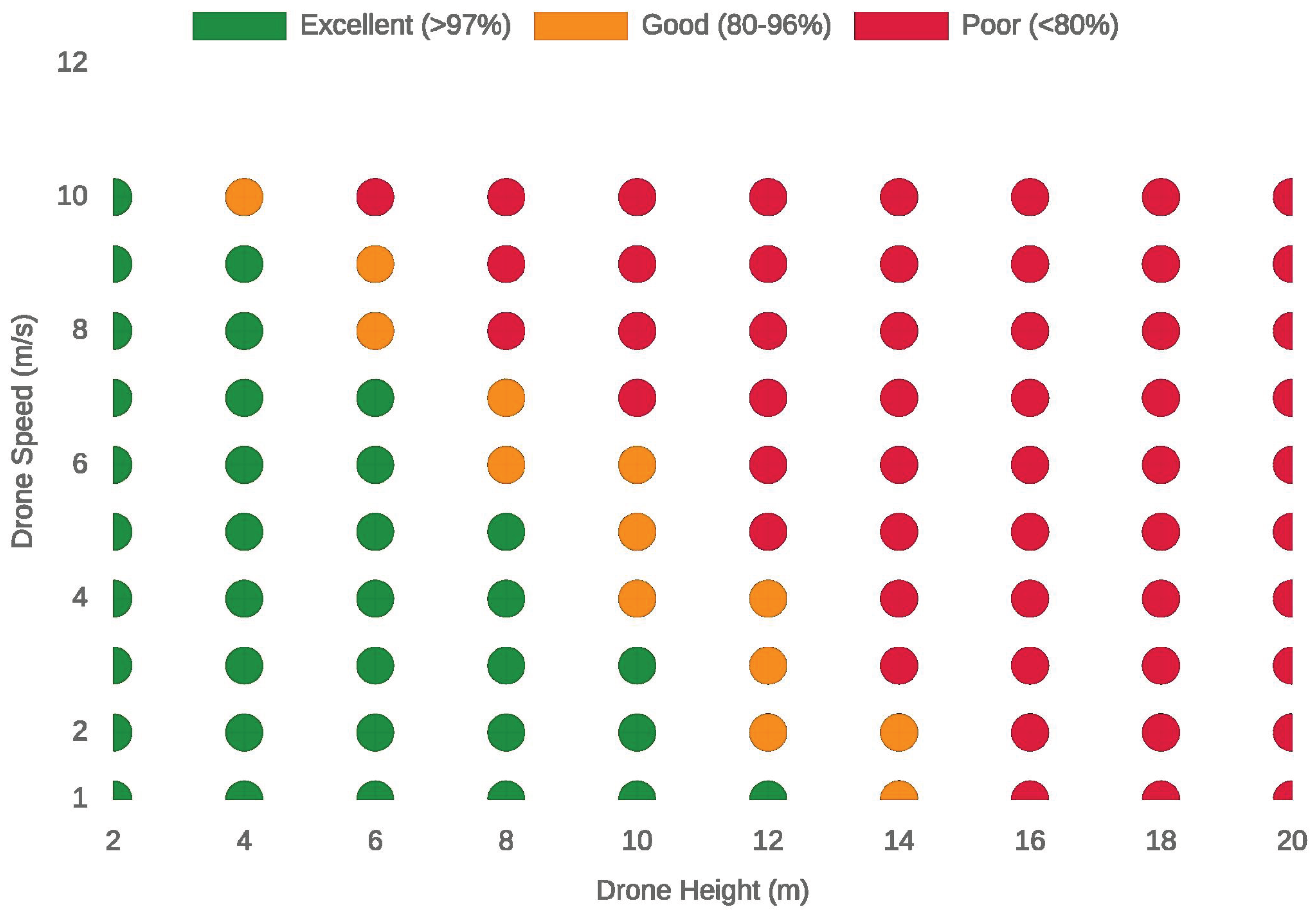
Finally, we combine both of the factors (Height and Speed) in one operational map as in Figure 6. Each colored circle represents an (height, speed) pair of the parameters and by color also performance quality:

•  Green: excellent seeding accuracy $\left(>97\%\right)$
•  Orange: acceptable or good performance $\left(80--90\%\right)$
•  Red: degraded performance $\left(<80\%\right)$

At lower altitudes (below 8 m) and moderate speeds (below 6 m/s), the hit probability remains high. The airflow perturbation is minimal, and the seed experiences less lateral drift and dispersion before impact. As height increases, or as drone speed exceeds 8–10 m/s, aerodynamic turbulence and timing error dominate. The seed’s descent time grows exponentially with height, exposing it to wind longer; meanwhile, at high speeds, along-track error caused by timing and heading misalignment expands the impact spread. The plot clearly highlights a safe operational corridor: a region of height–speed pairs where excellent recall can be maintained. With this map, operators can have a reference on how to setup their missions in mild winds and ensure accurate seeding.

5. Conclusion

In this study, we develop a general modeling and operational scheme for precision aerial sowing with variable wind conditions. By integrating analytical dispersion modeling with real-time presentation in an interactive dashboard, we turned intricate aerodynamic and stochastic activity into actionable operational advice. The proposed model relates observable flight characteristics such as height, speed the mean wind vector and turbulence intensity with a single probabilistic measure, $P_{\mathrm{hit}}$, which can be used for quantitative assessment as well as intuitive decision making support.

By analyzing example scenarios such as the low-recall tailwind alignment or high-recall crosswind conditions in this study, we showed that recall performance sensitively depends on wind alignment, drone speed, drone heading and flight altitude. By mapping a recall target $P^{★}$ to the feasible height–speed envelope $\mathcal{E}\left(P^{★}\right)$, the planner prescribes settings that maintain the required hit rate while transparently trading safety margin (height) against throughput (speed).

Apart from its analytical rigor, our dashboard makes environmental variability operational by defining data-driven limitations of flight to guarantee reliability and adaptability in the deployment zones. The future work will be to broaden the dashboard with autonomous adaptive control loops and to integrate field validation data in order to cover the simulation-to-reality gap. Collectively, the research provides a step towards field-scale sustainable accurate seeding operations.

References

- NASA Glenn Research Center. Terminal Velocity. Beginner’s Guide to Aeronautics, 2010. Available online. NASA. (accessed on 2025).
- Anderson, J.D. Fundamentals of Aerodynamics, 5 ed.; McGraw–Hill Education: New York, 2010. [Google Scholar]
- Clift, R.; Grace, J.R.; Weber, M.E. Bubbles, Drops, and Particles; Academic Press: New York, 1978. [Google Scholar]
- Vogel, S. Leaves in the Wind: Aerodynamics of Plant Propagules. American Journal of Botany 2009, 96, 1532–1545. [Google Scholar]
- Almasri, M.; Alhmiedat, T.; Namazi, M.A.; Ershath, M. Mangrove Propagule Seeding: Interactive dashboard for time-aware path planning with stochastic wind. 2025. Available online: https://aist-drone.netlify.app/ (accessed on Nov. 20 2025).
- Mohan, M.; et al. UAV-Supported Forest Regeneration: Current Trends, Research Directions, and Future Challenges. Remote Sensing 2021, 13, 2596. [Google Scholar] [CrossRef]
- Stamatopoulos, I.; et al. UAV-assisted seeding and monitoring of reforestation sites: A review. In Australian Geographer; 2024. [Google Scholar]
- Lysych, A.; et al. Design and Research Sowing Devices for Aerial Sowing of Forest Seeds with UAVs. Inventions 2021, 6, 83. [Google Scholar] [CrossRef]
- Hou, L.; et al. Design and experiment of a precision strip seeding UAV for rice. Transactions of the Chinese Society for Agricultural Machinery, (in Chinese). 2024. [Google Scholar]
- Liu, W.; et al. Evaluation method of rowing performance for UAV rice seeding. Computers and Electronics in Agriculture 2023, 205, 107600. [Google Scholar]
- Lee, Q.R.; et al. UAV-Based Precision Seed Dropping for Automated Reforestation. preprint 2025. [Google Scholar]
- Zhu, Y.; et al. Key parameters determination based on seed movement for UAV strip seeding. Computers and Electronics in Agriculture; 2025. [Google Scholar]
- Thomson, D.J. Criteria for the selection of stochastic models of particle trajectories in turbulent flows. Journal of Fluid Mechanics 1987, 180, 529–556. [Google Scholar] [CrossRef]
- Wilson, J.D.; Sawford, B.L. Review of Lagrangian stochastic models for trajectories in the turbulent atmosphere. Boundary-Layer Meteorology 1996, 78, 191–210. [Google Scholar] [CrossRef]
- Thomson, D.J.; Wilson, J.D. History of Lagrangian stochastic models for turbulent dispersion. In AGU Geophysical Monograph; American Geophysical Union, 2012. [Google Scholar]
- Emeis, S. Current issues in wind energy meteorology. Meteorological Applications 2014, 21, 803–819. [Google Scholar] [CrossRef]
- López-Villalobos, C.A.; et al. Analysis of the influence of the wind speed profile on wind power estimation. Energy Reports 2022, 8, 13056–13068. [Google Scholar] [CrossRef]
- Chin, G.Y. Two-Dimensional Measures of Accuracy in Navigational Systems. Technical report, U.S, 1987. Report; Department of Transportation. [Google Scholar]
- Spall, J.C.; Maryak, J.T. A Feasible Bayesian Estimator of Quantiles for Projectile Accuracy from Non-IID Data. Journal of the American Statistical Association 1992, 87, 471–480. [Google Scholar] [CrossRef]
- Rice, S.O. Mathematical Analysis of Random Noise. Bell System Technical Journal 1945, 24, 46–156. [Google Scholar] [CrossRef]
- Yakimenko, O.A. Statistical Analysis of Touchdown Error for Self-Guided Aerial Payload Delivery Systems. In Proceedings of the AIAA ADS, 2013. [Google Scholar]
- Zhang, J.; An, W. Assessing circular error probable when the errors are elliptical normal. Journal of Statistical Computation and Simulation 2012, 82, 565–586. [Google Scholar] [CrossRef]
- Lee, S.; Kim, J.; Ko, H.; Kim, S. Development and evaluation of an unmanned aerial vehicle seed-ball spreading system. Biosystems Engineering 2023, 226, 63–75. [Google Scholar]
- Wang, X.; Li, Y.; Zhang, Z.; Zhou, H. Field monitoring and wind tunnel study of wind effects on a long-span roof. Structural Control and Health Monitoring; 2020. [Google Scholar]
- Pope, S.B. Turbulent Flows; Cambridge University Press, 2000. [Google Scholar]
- Uhlenbeck, G.E.; Ornstein, L.S. On the Theory of the Brownian Motion. Physical Review 1930, 36, 823–841. [Google Scholar] [CrossRef]
- Stull, R.B. An Introduction to Boundary Layer Meteorology; Springer: Dordrecht, 1988. [Google Scholar]
- Khanjari, A.; Lundquist, J.K.; Pouragha, P. An analytical formulation for turbulence kinetic energy added by wind turbines based on LES. Wind Energy Science 2025, 10, 887–905. [Google Scholar] [CrossRef]
- Beard, R.W.; McLain, T.W. Small Unmanned Aircraft: Theory and Practice; Princeton University Press, 2012. [Google Scholar]
- Taylor, J.R. An Introduction to Error Analysis, 2 ed.; University Science Books, 1997. [Google Scholar]
- Bar-Shalom, Y.; Li, X.R.; Kirubarajan, T. Estimation with Applications to Tracking and Navigation; Wiley, 2001. [Google Scholar]
- Understanding GPS/GNSS: Principles and Applications, 3 ed.; Kaplan, E.D., Hegarty, C.J., Eds.; Artech House, 2017. [Google Scholar]
- van Diggelen, F. GPS accuracy: Lies, damn lies, and statistics. GPS World 1998, 9, 41–45. [Google Scholar]
- Rayleigh, Lord. On the resultant of a large number of vibrations of the same pitch and of arbitrary phase. Philosophical Magazine 1880, 10, 73–78. ser. 5. [Google Scholar] [CrossRef]
- Rice, S.O. Mathematical analysis of random noise. Bell System Technical Journal 1945, 24, 46–156. [Google Scholar] [CrossRef]
- Simon, M.K.; Alouini, M.S. Digital Communication over Fading Channels, 2 ed.; Wiley-IEEE Press, 2005. [Google Scholar]
- Kay, S.M. Fundamentals of Statistical Signal Processing. In Detection Theory; Prentice Hall, 1998; Vol. 2. [Google Scholar]
- White, F.M. Fluid Mechanics, 7 ed.; McGraw–Hill, 2011. [Google Scholar]
- Vogel, S. Life in Moving Fluids, 2 ed.; Princeton Univ. Press, 1994. [Google Scholar]
- Taylor, J.R. Classical Mechanics; University Science Books, 2005. [Google Scholar]
- Taylor, G.I. Diffusion by continuous movements. Proceedings of the London Mathematical Society 1921, 20, 196–212. [Google Scholar] [CrossRef]
- Tennekes, H.; Lumley, J.L. A First Course in Turbulence; MIT Press, 1972. [Google Scholar]
- Sawford, B.L. Reynolds number effects in Lagrangian stochastic models of turbulent dispersion. Physics of Fluids A 1991, 3, 1577–1586. [Google Scholar] [CrossRef]
Figure 1.
Vector Addition of Ground Velocity and Mean Drift.
Figure 2.
Wind-Aware Seeding Dashboard: Live Recall, Drift & Route Picks.
Figure 3.
Recall vs. Drone Speed at Different Height
Figure 4.
Error Budget vs. Speed: What Drives Placement Spread
Figure 5.
Recall vs. Height at Different Speeds
Figure 6.
Speed–Height Operating Map: Expected Seeding Recall
Disclaimer/Publisher’s Note: The statements, opinions and data contained in all publications are solely those of the individual author(s) and contributor(s) and not of MDPI and/or the editor(s). MDPI and/or the editor(s) disclaim responsibility for any injury to people or property resulting from any ideas, methods, instructions or products referred to in the content. |
© 2025 by the authors. Licensee MDPI, Basel, Switzerland. This article is an open access article distributed under the terms and conditions of the Creative Commons Attribution (CC BY) license (http://creativecommons.org/licenses/by/4.0/).
Copyright: This open access article is published under a Creative Commons CC BY 4.0 license, which permit the free download, distribution, and reuse, provided that the author and preprint are cited in any reuse.