Submitted:
23 December 2025
Posted:
25 December 2025
You are already at the latest version
Abstract
In February 2024, the European Union published its Industrial Carbon Management Strategy, setting ambitious goals for Carbon Capture and Storage (CCS), Carbon Cap-ture and Utilisation (CCU), and related technologies. Industrial decarbonisation will require a mix of solutions, CCUS, electrification, hydrogen and hydrogen-derived fuels, and energy efficiency, all dependent on affordable clean energy. Although carbon management technologies could contribute substantially to climate targets, their de-ployment has been slowed by technical barriers and public concerns. Sotacarbo created a research centre dedicated to developing and testing carbon capture, utilisation, and storage technologies. Within this framework, the new Sotacarbo Fault Laboratory (SFL) was designed to investigate gas migration in faults and to test monitoring systems ca-pable of detecting potential short- and long-term CO₂ leakages. This paper presents a preliminary study, including seismic full-waveform simulations for time-lapse surveys before and after CO₂ injection, and a suite of geophysical methods used to characterise the Matzaccara fault within the Eocene Sulcis Basin. The results of the application of integrated geophysical methods supported the selection of a safe and suitable injec-tion-well location and demonstrated the value of these methods for detailed fault characterisation in CCUS applications.
Keywords:
carbon capture
; Utilisation and Storage (CCUS)
; fault zone characterisation
; CO₂ monitoring and leakage detection
; multichannel seismics
; borehole geophysics
1. Introduction
The European Union’s strategy to combat global warming caused by the ongoing emission of greenhouse gases assigns Carbon Capture, Utilisation and Storage (CCUS) a crucial role in the EU Green Deal for the transition of energy-intensive industries and the power sector [1]. It is therefore essential to develop CCUS for industrial clusters, including system planning and shared infrastructure solutions. This should be achieved by demonstrating the full CCUS chain in the EU, focusing on reducing energy losses and capture costs, and implementing solutions for geological storage, both onshore and offshore. Onshore storage will support the management of decarbonisation strategies at the territorial level, while improving energy security, local economic activities, and safeguarding jobs across Europe. However, successful onshore storage also requires addressing specific technical and societal challenges: 1) development, testing, and demonstration of key technologies specifically adapted for onshore storage under real-world conditions; 2) contributing to the creation of a favourable environment for onshore storage across Europe through public acceptance. To support progress in geoscientific research and meet the global demand for safe, sustainable and secure CO₂ storage sites, both onshore and offshore, these challenges need to be thoroughly characterised and monitored to reassure the public and comply with EU legislation [2]. Methodologies and procedures should be developed to detect, attribute, and quantify any leakage from a CO₂ storage complex to the surface and into the environment. Research, innovation, testing, and verification require research infrastructures and services to address major challenges such as testing and engineering materials, drilling technologies, modelling and assessment of geomechanics and induced seismicity, and reservoir evaluation and management. Environmental monitoring technologies are also becoming increasingly important as the focus shifts from technical development to pilot projects, demonstrations, and real-world deployment of low-carbon geoenergies e.g., [3,4].
In this context, Sotacarbo, a research and development company (shareholders: Regional Government of Sardinia and ENEA, the Italian National Agency for New Technologies, Energy and Sustainable Economic Development) located in the south-western corner of Sardinia (Italy), in collaboration with the Universities of Cagliari and Rome "La Sapienza", OGS (National Institute of Oceanography and Applied Geophysics), INGV (National Institute of Geophysics and Volcanology),and RSE (Research on the Energy System), has launched an ambitious research programme funded by the Italian and Sardinian regional governments to explore the Sulcis coal basin as a potential site for testing technologies for CO₂ geological storage [5,6]. This includes methods for capturing carbon dioxide emissions from industrial processes and power generation plants (including biomass gasification systems), as well as research into ways of storing or utilising captured CO₂. For this reason, Sotacarbo’s facilities are integrated into the ECCSEL ERIC network (European Research Infrastructure for CO₂ Capture, Utilisation, Transport and Storage), which has covered the entire CCUS chain since its foundation. In particular, the Sotacarbo Fault Laboratory (SFL) facility has been designed specifically to study gas migration processes across faults and to test a wide range of monitoring technologies that are fundamental for detecting potential short- and long-term unwanted CO₂ leakages.
Various regional-scale studies on CCS (Carbon Capture and Storage) have been published in Italy to date, mostly focusing on identifying areas potentially suitable for CO₂ storage in saline aquifers [7,8,9,10,11,12]. This work presents a local case study analysed in detail, focusing on the Matzaccara normal fault, which was identified in the south-western part of the Sulcis coal basin and selected as the target tectonic structure for the SFL research activities. The Matzaccara fault was chosen as a test site because it exhibits the most recent tectonic activity among the faults identified in the southern Sulcis Basin and presents a near-surface fault plane. The investigations aimed to achieve two primary objectives: (1) to obtain detailed information about the fault's geometry and identify an ideal location for the CO₂ injection well, and (2) to validate geophysical monitoring methodologies to assess their effectiveness in detecting changes in subsurface conditions before, during, and after CO₂ injection. To address these objectives, the study integrated various geophysical data, including: 1) high-resolution reflection seismic data to understand the geometry, kinematics, displacement, age of activity, and areal extent of the fault; 2) borehole data to reconstruct the stratigraphy of the area affected by the fault; and 3) downhole measurements, including Vertical Seismic Profiling (VSP) and geoelectrical data acquired by sensors located along the well and at the surface.
The geophysical investigations conducted to date represent the baseline survey, aimed at defining the conditions of the site affected by the fault before CO₂ injection. Beyond this initial scope, the study demonstrates that integrating these geophysical methods is also crucial for evaluating and monitoring well integrity in CO₂ injection scenarios. The role of geophysics in Carbon Capture, Utilisation, and Storage (CCUS) applications is vital. These methods are essential for ensuring the safe and effective containment of CO₂ and the long-term sustainability of storage sites, thereby underpinning the success and reliability of CCUS initiatives.
2. Geology of the Sulcis coal basin
The Sulcis coal basin covers an onshore-offshore area of approximately 800 km² and is estimated to contain coal reserves exceeding one billion tonnes. The basement of the Sulcis basin consists of Palaeozoic metamorphic rocks and large volumes of granitoids related to the Hercynian Orogeny [13], locally overlain by Permo-Carboniferous terrigenous and volcanic complexes. Above these lies a predominantly Mesozoic carbonate succession of platform and basin environments [14]. This is followed by a Palaeogene transgressive-regressive sedimentary cycle [15] consisting of: i) a 30–50 m thick succession assigned to the Early Eocene Miliolitico Formation, composed of shallow-water fractured limestones rich in macroforaminifera [16,17], evolving into wackestone and mudstone rich in Miliolidae, deposited in lagoons, as well as in lacustrine and palustrine environments. The Miliolitico Formation has been proposed as the main reservoir for CO₂ injection [5,18]; ii) a rhythmic succession of siliciclastic to carbonate deposits up to 100 m thick, containing lignite intercalations and attributed to the Early Eocene Produttivo Formation [19]; iii) a Middle Eocene–Oligocene continental alluvial succession up to several hundred metres thick, known as the Cixerry Formation [15,20,21,22]. The uppermost part of the Sulcis basin succession consists of more than 900 m of Lower to Middle Miocene volcanic rocks, ranging from basaltic to rhyolitic composition. In the southern sector of the basin, the lower part of the volcanic sequence, which consists of andesites and basalts, is absent. The volcanic rocks are locally overlain by marine, lacustrine, alluvial and aeolian unconsolidated Quaternary sediments [23,24].
The study area is located in the southern sector of the Sulcis coal basin (see location and stratigraphy in Figure 1), where Sotacarbo has been granted a research permit for CCS-related studies. This area is affected by E–W, N–S, and NE–SW high-angle normal faults formed during Miocene extensional phases [6,18]. The main structure is the NNE-oriented Matzaccara Fault (Figure 1). The northern part of this structure was analysed using three high-resolution seismic profiles (Figure 1) to assess whether it could be an ideal target for studying fault behaviour in relation to fluid migration resulting from CO₂ injection.
Matzaccara Fault
The Matzaccara Fault was first identified through the interpretation of regional-scale seismic data acquired by OGS in the Monte Ulmus Exploration Permit in 2016 (Figure 1) [25]. Seismic data have provided an image of this tectonic structure: it exhibits normal kinematics and a listric fault plane dipping to the ESE (Figure 2). The fault affects the entire Eocene–Miocene volcano-sedimentary succession of the Sulcis coal basin and deforms the Quaternary alluvial deposits, which are characterised by a syntectonic wedge-shaped geometry, as shown by the seismic line in Figure 2.
Interpretation of the HR_1 high-resolution seismic profile (Figure 3) shows the architecture of the shallow part of the Matzaccara Fault. It consists of a fault zone with a SE-dipping main fault plane that has a maximum vertical offset of about 60–70 m. Two synthetic subsidiary faults are recognisable in its footwall, and a sub-vertical antithetic minor structure in the hanging wall.
The Matzaccara Fault is an ideal candidate for studying fault behaviour as a sealing barrier or as a preferential migration pathway for CO₂ movement, and for testing the sensitivity of geophysical instruments in monitoring the stored CO₂. A specific geophysical investigation at the SFL site revealed the presence of the fault within the first 200 metres below the surface using ambient noise tomography [26].
2. Materials and Methods
2.1. High- Resolution Multichannel Seismics
In June 2016, a high-resolution seismic survey was carried out in the study area to investigate the northern part of the Matzaccara Fault, previously identified on regional seismic lines. The aim was to define the characteristics of the fault (kinematics, geometry, displacement) down to a depth of 300 m, which was initially established for the CO₂ injection test. The survey consists of three NW-SE oriented parallel seismic profiles (HR_1, HR_2, and HR_3), spaced a few hundred metres apart (Figure 1). A Vibroseis source was used for seismic acquisition. The acquisition parameters (Table 1) were calibrated to achieve optimal resolution, considering the 300 m depth target and the drilled stratigraphy composed of Miocene volcanic rocks, which, due to the presence of fractures or voids, may cause scattering and attenuation of seismic waves, and are covered by Quaternary deposits.
The seismic data analysis revealed variability in signal-to-noise ratios across all profiles, influenced by subsoil response and noise from the nearby trunk road to Matzaccara. Processing efforts aimed to enhance signal-to-noise ratios by applying advanced techniques to attenuate both coherent and incoherent noise, and by increasing the amplitude and continuity of reflections. Tomographic inversion was performed using proprietary CAT3D software, while seismic data processing utilised ECHOS2011.3 and Seismic Unix. Two energisations per shot point were carried out and stacking of records at the same position preceded data processing. Processing steps included amplitude recovery, surface-consistent amplitude balancing, static corrections based on tomographic inversion, and various filtering techniques to improve signal quality. Dynamic corrections and migration using the Kirchhoff algorithm were applied to obtain stack and time-migrated sections (Figure 3).
Interpretation of the HR_1 high-resolution seismic profile, combined with stratigraphic information from the SFL monitoring well, enabled the identification of five seismic units separated by marker horizons (Figure 3). Unit 1 consists of Quaternary sedimentary deposits, while Units 2–5 form the Miocene volcanic succession.
- Unit 1: The shallowest unit is bounded at the top by the ground surface and at the base by the main high-amplitude marker horizon visible in the seismic profile. This unit displays a seismic facies characterised by sub-parallel, inclined, and undulating high-frequency reflectors with poor lateral continuity and low amplitude. Local downlap terminations against the marker reflector are evident. The thickness ranges from about 50 to 100 ms, corresponding to 30 to 60 m, assuming an interval velocity of 1200 m/s. The maximum thickness occurs in the hanging wall of the main fault plane of the Matzaccara fault zone.
- Unit 2: This unit comprises continuous high-amplitude reflectors deformed by the Matzaccara fault zone and secondary normal faults (Figure 3). The thickness is roughly constant, ranging between 30 and 50 ms, which corresponds to approximately 30 to 50 m, assuming an interval velocity of 2000 m/s for the entire volcanic succession crossed by the seismic profile.
- Unit 3: This unit consists of low-frequency, generally low-amplitude, sub-horizontal to inclined discontinuous reflectors (Figure 3). The minimum thickness, about 60 ms (60 m), is observed in the north-westernmost part of the line, where the inclined reflectors are truncated by the base of Unit 2. Elsewhere along the line, the thickness is roughly constant at about 80–110 ms (80–110 m).
- Unit 4: This unit consists of low-frequency, low- to high-amplitude, sub-horizontal discontinuous reflectors and has an approximately constant thickness of 100–110 ms (100–110 m) (Figure 3).
- Unit 5: The deepest unit consists of low-frequency, medium- to high-amplitude, sub-horizontal to undulating discontinuous reflectors. The maximum thickness, about 200 ms (200 m), is observed in the north-westernmost sector of the line.
2.2. Feasibility Study
The feasibility study aimed to assess the potential of geophysical methods for detecting injected CO₂ along the target fault and to determine the optimal parameters for planning the geophysical survey, thereby improving the site’s overall characterisation. This characterisation was essential to identify a suitable location for the planned injection well, complementing the monitoring well, to ensure proper CO₂ injection within the fault and to investigate its migration behaviour along the fault zone.
Elastic seismic full-waveform simulation was used to assess the effect of CO₂ injection on seismic waves propagation, particularly focusing on potential observations in a time-lapse acquisition before and after CO₂ injection. A 2D geological model was built based on the available data, and a preliminary, then revised, geological interpretation was formulated. The simulation was run with the vertical monitoring well (W1) and assumed a deviated injection well (W2) to intercept the fault within the planned 250 m drilling length. The wells are located on opposite sides of the interpreted fault (see Figure 4). The model had dimensions of 1000 × 500 metres and was discretised using square pixels with a side length of 0.5 metres. Both crosswell (CW) and surface acquisitions were simulated using seismic sources positioned in the vertical well and receivers placed every 1 m in the injection well for the CW acquisition, and at the surface. A Ricker wavelet with a 400 Hz cut-off frequency was used as the vertical synthetic source to remain within the Gassmann approximation. Several sources and CO₂ injection positions were tested, with the best results obtained from the source located at 250 m, which are presented here.

Theory
From a seismic perspective, the injected CO₂, which replaces water as the interstitial fluid, alters the bulk modulus of the saturated rock, thereby modifying the velocity at which compressional (P) waves propagate through the medium. In the model, the pore fluid in the pre-injection phase is water, which is subsequently replaced by CO₂ upon injection.
To compute the bulk and shear moduli (K_sat, μ_sat) of the porous fluid-saturated medium, Gassmann’s relations were applied. The Gassmann relations are derived under the assumption of low-frequency or quasi-static conditions, where fluid pressure within the pores has sufficient time to equilibrate across the pore space [28]. The validity of the Gassmann relation is typically controlled by Biot’s characteristic frequency (f_c), which separates low-frequency (quasi-static) from high-frequency (dynamic) behaviour and depends on the porosity and permeability of the rock and the dynamic viscosity of the fluid. For low- to medium-permeability rocks, f_c can range from 10 Hz to more than 1 kHz.
The fluid-saturated bulk and shear moduli are given by [29].
where ϕ is the porosity of the host rock, are the drained bulk and shear modulus, respectively, is the bulk modulus of the solid phase of the rock,
is the Biot’s coefficient and K_fluidis the bulk modulus of the pore fluid, which depends on the reservoir pressure and temperature conditions.
The complex compressional and shear saturated rock wave velocities are
from which, for homogeneous waves in isotropic media, we obtain the phase velocities
and the density of the porous medium is , where is the pore fluid density. At frequencies where the Gassmann relation is valid, we can expect a change in the P-wave velocity of the saturated rock in the area interested by the injection, which can result in changes in the seismic signal acquired before and post CO₂ injection.
Crosswell and surface numerical simulations
According to the information available at the time, the velocity model of the NW–SE line shown in Figure 4a was derived. In the crosswell simulation, the source was placed in the monitoring well at a depth of 250 m, and receivers were positioned every 1 m in the injection well. The injected CO₂ plume was considered at a depth of about 190 m in the injection well (W2). The radius of the simulated sphere was calculated as if 5.5 tonnes of CO₂ were injected (radius = 6 m, Figure 4b). The geophysical properties of the host layer were set as follows: P-wave velocity of the host rock solid phase V_(P_s) = 3800 m/s, density computed with Gardner’s relation ρ_s = 2300 kg/m³, compressional to shear wave velocity ratio of 2, Biot’s coefficient α = 0.36, and porosity ϕ = 0.09. The density, acoustic velocity, and bulk modulus of the fluids (water and CO₂) were computed at the corresponding reservoir pressure and temperature conditions (P = 30 atm, T = 18°C), using the CoolProp codes [30] based on the thermophysical database provided by the National Institute of Standards and Technology (NIST).
Elastic full-waveform propagation in the crosswell configuration was simulated, and the resulting synthetic pressure components are shown in Figure 5, using consistent amplitude normalisation across the three panels. The seismograms show the signals after CO₂ injection (Figure 5a), before injection (Figure 5b), and the difference between the two is shown in Figure 5c. Although the amplitude of the difference signal is relatively low compared to the full synthetics, clear reflections from the boundaries of the CO₂ plume are visible in the receivers below 200 m depth in Figure 5a and become particularly evident in the difference panel (Figure 5c).
The synthetic signals recorded at the surface (Figure 6) were also acquired from the source located at a depth of 250 m in the monitoring well. As expected, the configuration with surface receivers, while keeping all other modelling parameters unchanged, proved less effective than the crosswell configuration in detecting changes associated with the CO₂ plume. The seismograms after injection (Figure 6a), before injection (Figure 6b), and their difference (Figure 6c) are displayed using the same amplitude normalisation, but with a higher global gain compared to the crosswell configuration (Figure 5). The difference signal is barely visible, particularly for receivers located to the right of the plume. In Figure 6c, the presence of CO₂ affects the first arrivals, but the effect on the reflection is not visually detectable in this type of acquisition geometry. These results suggest that seismic monitoring in a crosswell configuration is preferable, especially if the injection well is equipped with permanent instrumentation such as Distributed Acoustic Sensing (DAS), which provides highly dense spatial resolution e.g., [31,32].
2.3. Borehole Geophysical Study
Following the modelling of the initial feasibility study and the high-resolution seismic investigations, borehole seismic surveys were conducted to characterise the Matzaccara fault and its surrounding area as a baseline for CO₂ injection test purposes for SFL.
The opportunity to perform borehole geophysical surveys arose from the presence of the monitoring well W1 (SFL monitoring well) close to the main fault (Figure 7). The vertical well W1 was cased to a depth of 250 m with a fibreglass casing, which is also suitable for geoelectrical surveys such as Electric Resistivity Tomography (ERT) [33]. Vertical Seismic Profiles (VSP) are geophysical measurements made in a wellbore with geophones positioned at depth inside the wellbore and a seismic source at the surface, typically near the well. The seismic source generates acoustic waves that are recorded by the geophones in the well. VSPs offer significant advantages over surface seismic surveys: VSP data have higher resolution, as the wave path is shorter (receivers are in the well), and they provide a direct correspondence between time and depth, which is used to calibrate the surface seismic data. Furthermore, VSPs provide interval velocities in depth along the well, giving indications about the type of formations encountered from a seismic perspective. The data collected in 2019–2020 by VSP, jointly analysed with resistivity data from the geoelectric survey, provided useful indications on the possible location of the injection well, which was planned to be drilled in 2023.
The geophysical surveys consisted of:
- Two near-offset Vertical Seismic Profiles (VSP);
- Multi-offset VSP (several VSP surveys with the source moving along offset) in well W1 and in a shallower piezometric well 65 m from W1;
- A geoelectrical survey with electrodes located both in the well and at the surface.
The results of the two near-offset VSPs from the vertical component data, the resistivity model from ERT, and the joint data integration of these two complementary methodologies are described below.
2.3.1. Near-Offset VSPs
The two near-offset VSPs were conducted in February 2020 at 10 m (SP 510) and 30 m (SP 530) offset south-east from well W1, respectively (Figure 7). The surveys were performed using an Avalon 3C geophone, capable of recording the vertical and horizontal components of the different wavefields, from 5 m to 240 m depth along the well. The source was an IVI Minivib Vibroseis, driven by a Seismic Source Force III control system, which includes encoder and decoder units installed on the Vibroseis and in the control cabin, respectively, where the time break signal for the sweep start is delivered and the reference signals (the pilots) are fed into the acquisition system. The Minivib operated in P mode, using a sweep from 10 Hz to 320 Hz. The spatial sampling of the receivers in the well was 2.5 m.
The VSP 510 is strongly dominated by tube waves (Figure 8a), generated by the source very close to the well. Starting from the picking of the first arrivals of the total wavefield, the one-way traveltime (OWT) upgoing wavefield, representing the reflections from the subsurface, was recovered by wavefield separation (Figure 8b). The wavefield separation enhances the upgoing events and partially attenuates the tube waves. In addition, we applied an F-K filter to further attenuate the tube waves and better highlight the reflections. The total wavefield of VSP 530 is less dominated by tube waves, as the source was located farther from well W1 (Figure 8c). Figure 8d shows the corresponding OWT upgoing wavefield.
Using the first arrivals from the VSP data, the interval velocities of the geological formations across the well were calculated. Figure 9 illustrates the interpretation of formation tops in relation to changes in the velocity function with depth.
Figure 9 and Figure 10 show that three of the interpreted formation tops from the calculated interval velocities align with the reflections observed in the two-way traveltime (TWT) VSP 510 upgoing wavefield. However, the quality of data for shallower reflections is compromised by the presence of unconsolidated sediments or weathering, making reliable interpretation difficult. Figure 10 also presents the TWT corridor stack derived from the data, which visually enhances the reflections. The VSP data facilitate the calibration of reflection seismic, linking the TWT reflectors of the stack section to the corresponding depths. This enables comparison of the VSP results with the HR1 reflection seismic stack time section (Figure 10), which is closest to well W1 (see map in Figure 1). The stack section was divided, and the corridor stack was positioned at the corresponding projected well location on the line (Figure 11). Using the time-depth correspondence in the VSP from Figure 10, the depth of the signal in time can be directly determined. This information is shown in Figure 11, where the coloured circles along the corridor stack indicate the depth of the selected reflectors in the stack section. The formation at the depth of the green circle is interpreted as the top of Comenditi, the one at the depth of the red circle as the top of Nuraxi, and the one at the depth of the yellow circle as the top of Monte Crobu. The blue signal has not been assigned to a specific top formation, as it appears clearly in the corridor stack from the VSP but cannot be resolved by the seismic data due to its very thin thickness.
2.3.2. Electric Resistivity Tomography (Ert)
Integration of different methodologies increases the reliability of the results. For this purpose, in addition to the two seismic methods (surface seismic and VSP), an electrical survey was conducted. Electrical resistivity tomography (ERT) is a non-invasive geophysical method for investigating the subsurface by examining the electrical properties of the geological formation. It assumes that different entities, such as minerals, solid bedrock, sediments, air-filled and water-filled structures, exhibit detectable contrasts in electrical resistivity compared to the host medium [34].
In December 2019, 2D and 3D ERT surveys were carried out, both surface and surface-borehole, in the SFL, where observation well W1 was already equipped with 48 electrodes spaced at approximately 5 m intervals [33]. The first four electrodes were not used in the acquisition due to the presence of steel casing in the upper part, while the remainder of the well has a fibreglass casing, as previously described.
The 2D surface profile, oriented NW-SE and 920 m in length, consists of 48 electrodes spaced 20 m apart and follows the seismic lines HR_1 (Figure 12).
Three different geometries were used for the 2D acquisition:
1) Wenner–Schlumberger 2D surface profile,
2) Wenner–Schlumberger along the borehole,
3) Surface-to-borehole Dipole–Dipole between the 2D surface profile and the borehole.
Data inversion
The collected data were inverted by OGS using ERTLab64 software by Geostudi Astier, for both single acquisitions and combined datasets. The primary objective at this stage of the project was to enhance the available information in the area between the observation well and the planned injection well. Useful information was obtained exclusively from the 2D and 3D surface surveys, as the data inversions from borehole electrodes produced unreliable higher resistivity values compared to surface data, obscuring the resistivity values of deeper formations.
A preliminary 1D profile was constructed from resistivity data collected across the well. To validate this profile, it was compared with both the VSP TWT upgoing wavefield and the velocity profile (Figure 13). The joint interpretation shows good correspondence between changes in resistivity and the velocity function (on the right), confirmed by changes in the lithostratigraphy identified by the VSP interpretation (on the left).
The comparison between the 2D resistivity profile and the HR_1 seismic section (Figure 14) shows a strong correlation between resistivity variations and the geological interpretation. Notably, in the Matzaccara fault zone, a distinct shift in the resistivity pattern is observed. Higher resistivity values are present to the left of the monitoring well, while these values decrease towards the right, or southeast. The topmost layer corresponds to Quaternary alluvial deposits (Figure 1), and the variation in resistivity is likely not due to changes in lithology but rather to the presence of the fault. In fault zones, particularly on the hanging wall, increased fracturing is common, leading to higher porosity compared to the surrounding rock. This enhanced porosity facilitates fluid accumulation, which may result in the formation of a "fault gouge" – a zone of finely crushed rock material within the fault. Fault gouge typically exhibits lower resistivity than the surrounding rock due to its finer grain size, higher porosity, and greater likelihood of being saturated with conductive fluids. This observation supports the conclusion that the Matzaccara fault has been recently active, influencing the characteristics of the Quaternary deposits.
3. Results
By integrating geophysical and well-log data with geological information from the geological map sheet no. 564 “Carbonia” [23,24] and the SFL monitoring well, the seismic section was interpreted as follows:
− Unit 1: represents the Quaternary alluvial deposits.
− Unit 2: represents the uppermost part of the volcanic sequence, deformed by the Matzaccara fault zone and secondary normal faults. This unit was correlated with the Langhian Paringianu Rhyolites Formation, which consists of pyroclastic fall and flow deposits (tuffs and lapilli).
− Unit 3: this seismic unit has been associated with several Langhian pyroclastic volcanic formations, such as the Hyperalkaline Rhyolites of Mt. Ulmus, Cala Saboni Comendites, and Matzaccara Dacites.
− Unit 4: this unit is associated with the Langhian Nuraxi Rhyolites Formation, consisting of densely welded pyroclastic flow deposits.
− Unit 5: the deepest unit, has been associated with the Burdigalian-Langhian Mt. Crobu Rhyolites Formation, composed of densely welded pyroclastic deposits.
Injection well
The previously described site characterisation provided detailed information for the design of the injection well (Figure 15). Unlike the plan in the feasibility study simulation, the injection well was drilled vertically; however, this did not affect the validity of the modelling results for the geophysical studies conducted. The well was drilled in the hanging wall of the fault, passing through the Holocene sandy deposit to a depth of 47 m and reaching the top of the upper rhyolitic rock (Paringianu Fm.). The fault was intercepted at a depth of about 100 m. The injection well is equipped with a 5½’’ (140 mm) fibreglass casing (selected to prevent electrical interference with the ERT cables installed outside the casing), which houses the injection pipes and allows monitoring probes to be introduced into the well. In parallel, a fibre optic cable was run from the casing shoe to the surface to enable monitoring of gas migration in the rock above the injection point. Standard class G cement was used to cement the casing and the cable in place, isolating groundwater and minimising potential leakage pathways along interfaces between well casings and geological formations and along cables, thus ensuring that CO₂ only leaks through the soil and the fault. Pressure, temperature, geoelectrical, geochemical and seismic data can be collected, processed and analysed during the injection tests. In addition, two downhole pressure and temperature transmitters (DPTT) have been installed to provide accurate measurements at the bottom of the well in the injection zone (Figure 15).
4. Discussion and Conclusion
This study demonstrates the use of integrated geophysical techniques to characterise the CO₂ Sulcis Fault Lab (SFL) test site, located in the southern part of the Sulcis coal basin in Sardinia. The site was selected to investigate the behaviour of CO₂ in the presence of faults. It is characterised by a several hundred metre thick Miocene volcanic sequence, a type of rock that generally produces a weak seismic response. Therefore, a feasibility study was conducted to assess the potential of geophysical methods to detect injected CO₂ along the target fault, the Matzaccara Fault, identified by regional-scale seismic reflection profiles, and to determine the optimal acquisition parameters for survey planning, thereby improving overall site characterisation. The regional-scale seismic profiles show that the fault also affects the Quaternary deposits. High-resolution seismic profiles acquired along the fault trace were essential to define the kinematics, geometry, and displacement associated with the Matzaccara Fault. The seismic investigation reached depths of approximately 300 m, slightly beyond the planned CO₂ injection depth. Five seismic units were identified. The shallowest consists of Quaternary deposits overlying the Miocene volcanic sequence, which is mainly composed of rhyolites, as well as comendites and dacites. The data provided a detailed image of the architecture of the Matzaccara Fault zone, which consists of a SE-dipping main fault plane with a normal offset of approximately 50–60 m, two synthetic minor faults in the footwall, where the SFL monitoring well is located, and a sub-vertical antithetic structure in the hanging wall. Interpretation of the seismic lines showed that the Matzaccara Fault is the most recent fault in the southern Sulcis basin. Therefore, by studying its behaviour in relation to CO₂ injection, it will be possible to hypothesise the behaviour of the older tectonic structures in the area. Moreover, the seismic data provided crucial information for subsequent investigations, including the definition of acquisition parameters for borehole geophysics and planning the injection well. VSP data provided interval velocities for the geological formations intersected by the well. These velocities enabled the construction of a time–depth relationship used to align seismic reflections (in two-way travel time) with the lithological tops identified in well W1. A corridor stack generated from the upgoing VSP wavefield enhanced reflection visibility and facilitated comparison with reflections interpreted on the HR-1 seismic section, allowing the tops of the Comenditi, Nuraxi, and Monte Crobu volcanic formations to be confidently assigned. ERT tomography profiles revealed distinct resistivity patterns on either side of well W1. Lower resistivity values were observed to the southeast, towards the planned injection well. This trend is consistent with the geological interpretation of seismic line HR-1, as confirmed by integrating the seismic and 2D resistivity sections. The resistivity distribution supports the presence and activity of the Matzaccara Fault. The integrated geophysical investigations at the SFL site provided the essential framework for designing, positioning, and instrumenting the injection well. Although the initial feasibility study assumed a deviated well trajectory, drilling a vertical well did not compromise the modelling results. Simulations showed that the detectability of CO₂-induced seismic velocity changes remains high in a vertical configuration, particularly when the injection well is incorporated into a crosswell monitoring scheme. The modelling also underscored the importance of permanent downhole instrumentation, especially fibre-optic cables for DAS measurements, to detect small velocity perturbations associated with CO₂ migration. The drilled injection well has encountered the fault at a depth of about 100 m, confirming the validity of the geophysical analysis. The upcoming experiments are expected to provide more details and numerical data required to further improve the model and develop advanced monitoring tools.
The study demonstrates that only a fully integrated geophysical approach can meet the requirements for the characterisation and long-term monitoring of fault behaviour in relation to CO₂ storage, which is one of the major challenges in CCS technology.
Author Contributions
“Conceptualization, V.V., C.B. D.C.; methodology, V.V. and C.B.; software, M.F., P.C., F.A., M.G., C.B.; investigation, M.G., F.A., A.S., M.G., E.F., D.C., F.M; data curation, D.C., B.F., P.C., F.A., M.G., C.B., F.M.,F.P.; writing—original draft preparation, V.V.,C.B., D.C., E.B., M.G.; writing—review and editing, V.V., C.B., D.C.; visualization, C.B., V.V., D.C., B.F., P.C., F.A., M.G., A.P., A.P.2, ;supervision, V.V. All authors have read and agreed to the published version of the manuscript
Funding
This research was funded by the European Union’s Horizon 2020 research and innovation programme under Grant Agreement No. 653718 (ENabling Onshore CO₂ Storage in Europe—ENOS).
Data Availability Statement
The high-resolution seismic profiles reported in the manuscript and acquired by OGS are available in SEGY format on request from the corresponding author. Borehole geophysical data (VSP and Electrict Resistivity Tomography) are collected by OGS and can be made available upon request referring to the corresponding author.
Acknowledgments
The authors acknowledge the technical staff of OGS for the acquisition of the geophysical data presented in this work.
Conflicts of Interest
The authors declare no conflicts of interest.
References
- IEA 2023, World Energy Investment 2023 Report. IEA, Paris. Available online: https://www.iea.org/reports/world-energy-investment-<b>2023</b> (accessed on 5/11/2025).
- Directive 2009/31/EC of the European Parliament and of the Council of 23 April 2009 on the geological storage of carbon dioxide and amending Council Directive 85/337/EEC, European Parliament and Council Directives 2000/60/EC, 2001/80/EC, 2004/35/EC, 2006/12/EC, 2008/1/EC and Regulation (EC) No 1013/2006.
- Stork, A.; Poletto, F.; Draganov, D.; Janssen; Hassing, S.; Meneghini, F.; Böhm, G.; David, A.; Farina, B.; Schleifer, A.; Durucan, S.; Brynjarsson, B.; Hjörleifsdóttir, V.; Perry, W.; van Otten, G.; Barnhoorn, A.; Wolf, K. H.; Korre, A.; Bos, J.; Bellezza, C.; Chalari, A.; Obermann, A.; Sánchez-Pasto, P. Monitoring CO₂ injection with passive and active seismic surveys: Case study from the Hellisheiði geothermal field, Iceland. In Proceedings of the 16th Greenhouse Gas Control Technologies Conference (GHGT-16), Available at SSRN. Lyon, France, 23-27 October 2022. [Google Scholar] [CrossRef]
- Bellezza, C.; Barison, E.; Poletto, F.; Meneghini, F.; Schleifer, A.; Stork, A.; Draganov, D.; van den Berg, J.; van Otten, G.; Durucan, S.; Korre, A.; Hjörleifsdóttir, V.; Brynjarsson, B. Time-Lapse Seismic Monitoring of CO₂ Injection and Storage at the Hellisheiði Geothermal Field, Iceland. In Proceedings of the 17th Greenhouse Gas Control Technologies Conference (GHGT-17), Calgary, Canada, 20-24 October 2024; Available online: https://ssrn.com/abstract=5010204. [CrossRef]
- Fais, S.; Ligas, P.; Cuccuru, F.; Maggio, E.; Plaisant, A.; Pettinau, A.; Casula, G.; Bianchi, M.G. Detailed petrophysical and geophysical characterization of core samples from the potential caprock-reservoir system in the Sulcis Coal Basin (Southwestern Sardinia–Italy). Energy Procedia 2015, 76, 503–511. [Google Scholar] [CrossRef]
- Tartarello, M.C.; Plaisant, A.; Bigi, S.; Beaubien, S.E.; Graziani, S.; Lombardi, S.; Ruggiero, L.; De Angelis, D.; Sacco, P.; Maggio, E. Preliminary results of geological characterization and geochemical monitoring of Sulcis Basin (Sardinia), as a potential CCS site. Energy Procedia 2017, 125, 549–555. [Google Scholar] [CrossRef]
- Buttinelli, M.; Procesi, M.; Cantucci, B.; Quattrocchi, F.; Boschi, E. The geo-database of caprock quality and deep saline aquifers distribution for geological storage of CO₂ in Italy. Energy 2011, 36(5), 2968–2983. [Google Scholar] [CrossRef]
- Donda, F.; Volpi, V.; Persoglia, S.; Parushev, D. CO₂ storage potential of deep saline aquifers: The case of Italy. Int. J. Greenh. Gas Control 2011, 5, 327–335. [Google Scholar] [CrossRef]
- Civile, D.; Zecchin, M.; Forlin, E.; Donda, F.; Volpi, V.; Merson, B.; Persoglia, S. CO₂ geological storage in the Italian carbonate successions. Int. J. Greenh. Gas Control 2013, 19, 101–116. [Google Scholar] [CrossRef]
- Donda, F.; Civile, D.; Forlin, E.; Volpi, V.; Zecchin, M.; Gordini, E.; Merson, M.; De Santis, L. The northernmost Adriatic Sea: A potential location for CO₂ geological storage? Mar. Pet. Geol. 2013, 42, 148–159. [Google Scholar] [CrossRef]
- Volpi, V.; Forlin, E.; Baroni, A.; Estublier, A.; Donda, F.; Civile, D.; Caffau, M.; Kuczynsky, S.; Vincké, O.; Delprat-Jannaud, F. Evaluation and characterization of a potential CO₂ storage site in the south Adriatic offshore. Oil Gas Sci. Technol. 2015, 70(4), 695–712. [Google Scholar] [CrossRef]
- Volpi, V.; Forlin, E.; Donda, F.; Civile, D.; Facchin, L.; Sauli, S.; Merson, B.; Sinza-Mendieta, K.; Shams, A. Southern Adriatic Sea as a potential area for CO₂ geological storage. Oil Gas Sci. Technol. 2015, 70(4), 713–728. [Google Scholar] [CrossRef]
- Carmignani, L.; Pertusati, P.C.; Barca, S.; Carosi, R.; Di Pisa, A.; Gattiglio, M.; Musumeci, G.; Oggiano, G. Struttura della catena ercinica in Sardegna. In Guida all'escursione; Centrooffset Siena: Siena, Italy, 1992; p. 1-177 pp. 1-177. [Google Scholar]
- Costamagna, L.; Barca, S. The Germanic Triassic of Sardinia (Italy): a stratigraphic, depositional and palaeogeographic review. Riv. ital. paleontol. stratigr. 2022, 108, 67–100. [Google Scholar] [CrossRef]
- Costamagna, L.G.; Schäfer, A. Evolution of a Pyrenean molassic basin in the Western Mediterranean area: The Eocene–Oligocene Cixerri Formation in Southern Sardinia (Italy). Geol. J. 2018, 53(1), 424–437. [Google Scholar] [CrossRef]
- . [CrossRef]
- Fanni, S.; Murru, M.; Salvadori, A.; Sarria, E. Nuovi Dati Strutturali Sul Bacino Del Sulcis. L’Industria Mineraria 1982, 4, 25–31. [Google Scholar]
- Murru, M.; Salvadori, A. Ricerche stratigrafiche sul bacino del Sulcis (Sardegna sudoccidentale). I depositi continentali paleocenici della Sardegna meridionale ed il loro significato paleoclimatico. Geol. Rom. 1987, 26, 149–165. [Google Scholar]
- Bigi, S.; Tartarello, M.C.; Ruggiero, L.; Graziani, S.; Beaubien, S.; Lombardi, S. On-going and future research at the Sulcis site in Sardinia, Italy – characterization and experimentation at a possible future CCS pilot. Energy Procedia 2017, 114, 2742–2747. [Google Scholar] [CrossRef]
- Murru, M.; Ferrara, F.; Da Pelo, S.; Ibba, A. The Paleocene-Middle Eocene deposits of Sardinia (Italy) and their paleoclimatic significance. C. R. Geosci. 2003, 335, 227–238. [Google Scholar] [CrossRef]
- Barca, S.; Maxia, C.; Palmerini, V. Sintesi sulle attuali conoscenze relative alla “Formazione del Cixerri” (Sardegna sud-occidentale). Boll. Serv. Geol. It 1973, 94, 307–318. [Google Scholar]
- Barca, S.; Palmerini, V. Contributo alla conoscenza degli ambienti di sedimentazione relativi alla “Formazione del Cixerri” (Sardegna sud-occidentale). Boll. Soc. Sarda Sci. Nat. 1973, VII(XII), 13–47. [Google Scholar]
- Barca, S.; Costamagna, L.G. New stratigraphic and sedimentological investigations on the Middle Eocene–Early Miocene continental successions in southwestern Sardinia (Italy): Paleogeographic and geodynamic implications. C. R. Geosci. 2010, 342-2, 116–125. [Google Scholar] [CrossRef]
- Deiana, G.; Carmignani, L.; Orrù, P.; Sale, V.; Pintus, C.; Pisanu, G.; Ulzega, A.; Pasci, S. Note Illustrative della Carta geologica d'Italia alla scala 1:50.000, F. 564 Carbonia. Servizio Geologico d'Italia – ISPRA 2012. [Google Scholar] [CrossRef]
- Carta Geologica d’Italia alla scala 1:50.000, Foglio 564 Carbonia. In Servizio Geologico d’Italia - ISPRA; 2012. [CrossRef]
- Plaisant, A.; Maiu, A.; Maggio, E.; Pettinau, A. Pilot-scale CO₂ sequestration test site in the Sulcis Basin (SW Sardinia): preliminary site characterization and research program. Energy Procedia 2017, 114, 4508–4517. [Google Scholar] [CrossRef]
- Anselmi, M.; Saccorotti, G.; Piccinini, D.; Giunchi, C.; Paratore, M.; De Goria, P.; Buttinelli, M.; Maggio, E.; Plaisant, A.; Chiarabba, C. Microseismic assessment and fault characterization at the Sulcis (South-Western Sardinia) field laboratory. Int. J. Greenh. Gas Control 2020, 95, 102974. [Google Scholar] [CrossRef]
- Tedde, F.; Maiu, A.; Plaisant, A.; Pettinau, A. Experimental comparison between dynamic and static parameters for volcanic rocks in Sulcis basin (Italy). J. Appl. Geophys. 2023, 217, 105181. [Google Scholar] [CrossRef]
- Berryman, J.G. Origin of Gassmann’s equations. Geophysics 1999, 64(5), 1627–1629. [Google Scholar] [CrossRef]
- Farina, B.; Parisio, F.; Poletto, F. A seismic-properties and wave-propagation analysis for the long-term monitoring of supercritical geothermal systems. Geothermics 2022, 104, 102451. [Google Scholar] [CrossRef]
- Bell, I.H.; Wronski, J.; Quoilin, S.; Lemort, V. Pure and pseudo-pure fluid thermophysical property evaluation and the open-source thermophysical property library CoolProp. Ind. Eng. Chem. Res. 2014, 53(6), 2498–2508. [Google Scholar] [CrossRef] [PubMed]
- Meneghini, F.; Poletto, F.; Bellezza, C.; Farina, B.; Draganov, D.; Van Otten, G.; Stork, A.L.; Böhm, G.; Schleifer, A.; Janssen, M.; Travan, A.; Zgauc, F.; Durucan, S. Feasibility Study and Results from a Baseline Multi-Tool Active Seismic Acquisition for CO₂ Monitoring at the Hellisheiði Geothermal Field. Sustainability 2024, 16, 7640. [Google Scholar] [CrossRef]
- Bellezza, C.; Barison, E.; Farina, B.; Poletto, F.; Meneghini, F.; Böhm, G.; Draganov, D.; Janssen, M.T.G.; van Otten, G.; Stork, A.L.; Chalari, A.; Schleifer, A.; Durucan, S. Multi-Sensor Seismic Processing Approach Using Geophones and HWC DAS in the Monitoring of CO₂ Storage at the Hellisheiði Geothermal Field in Iceland. Sustainability 2024, 16, 877. [Google Scholar] [CrossRef]
- Mattioli, L.; Conte, A. Programma di perforazione pozzo verticale Progetto “SOTACARBO FAULT LAB”. Documento Tecnico di Progetto del pozzo verticale di Monitoraggio SOTACARBO FAULT LAB 2019, 77 pp. [Google Scholar]
- Pánek, T.; Margielewski, W.; Táborík, P.; Urban, J.; Hradecký, J.; Szura, C. Gravitationally induced caves and other discontinuities detected by 2D electrical resistivity tomography: case studies from the Polish Flysch Carpathians. Geomorphology 2010, 123, 165–180. [Google Scholar] [CrossRef]
Figure 1.
– Simplified geological map of the Sulcis coal basin (Carbosulcis, 1993) (left), with the location of the Matzaccara Fault. The position of the NE-SW oriented regional seismic profile 3 (blue solid line) and of the three NW-SE oriented high-resolution seismic lines (blue dashed lines), which were acquired in 2016, used to characterize the Matzaccara Fault is also reported, together with the location (black circle) of the SFL monitoring well [27]. On the right side the simplified stratigraphic column of the Sulcis basin is shown and the detailed stratigraphy of the SFL monitoring well used to interpret the seismo-stratigraphy of the high-resolution seismic profiles.
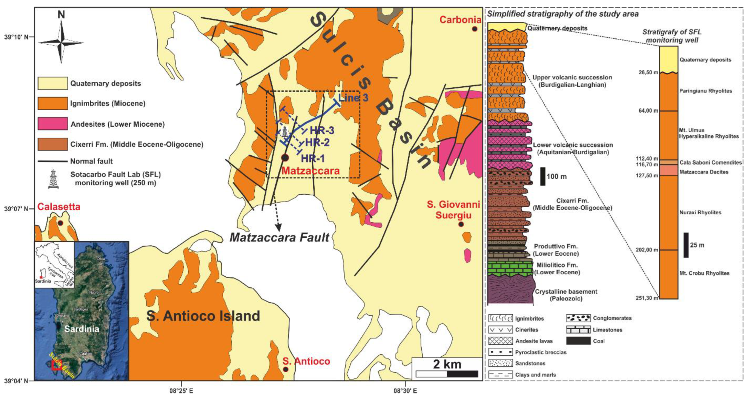
Figure 2.
– Interpretation of multichannel seismic line 3, which images the listric fault plane of the Matzaccara normal fault (location in Figure 1). The wedge-shaped geometry of the Quaternary deposits and a graben structure are visible.
Figure 2.
– Interpretation of multichannel seismic line 3, which images the listric fault plane of the Matzaccara normal fault (location in Figure 1). The wedge-shaped geometry of the Quaternary deposits and a graben structure are visible.
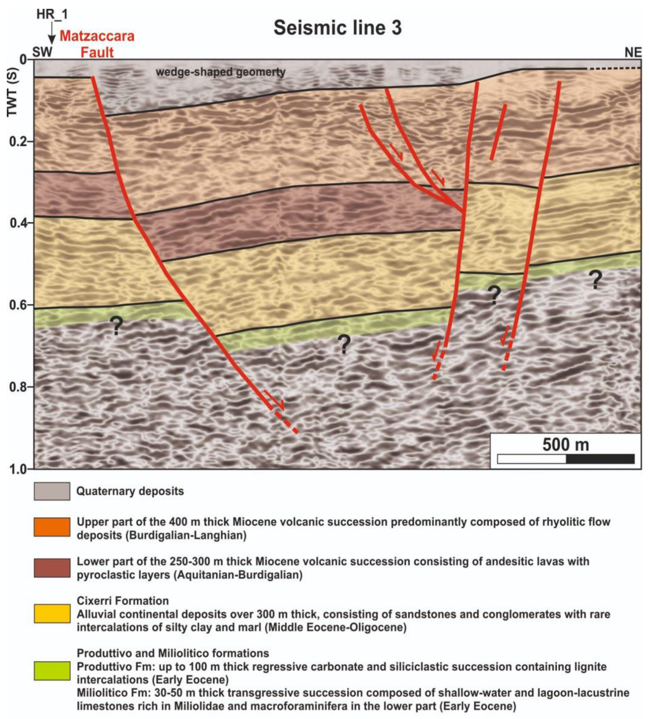
Figure 3.
– uninterpreted and interpreted HR_1 high resolution seismic profile crossing the Matzaccara Fault Zone (location in Figure 1). Vertical scale is expressed in seconds two-way time (TWT).
Figure 3.
– uninterpreted and interpreted HR_1 high resolution seismic profile crossing the Matzaccara Fault Zone (location in Figure 1). Vertical scale is expressed in seconds two-way time (TWT).
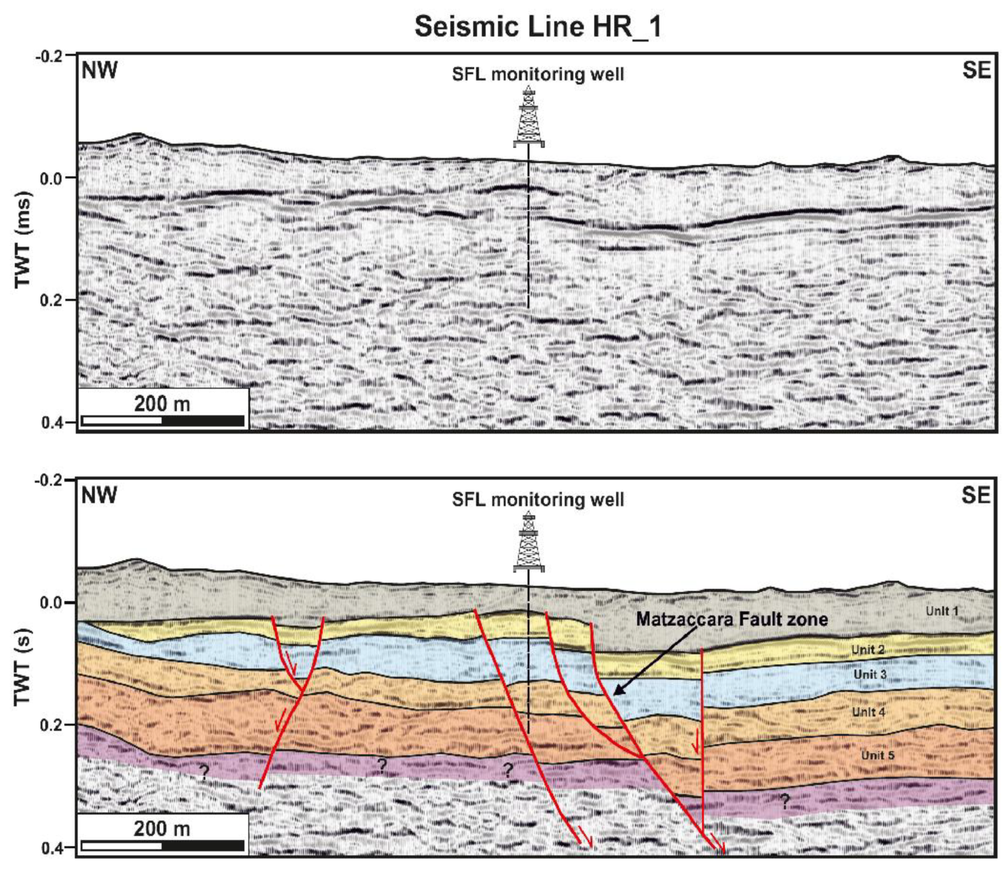
Figure 4.
- 2D models used to simulate waveform propagation before (a) and after (b) injection. The colorbar is set to show the VP velocity variation in the modelled CO₂ sphere in (b) (depth 190 m, 6m radius circle close to the deviated well and the interpreted fault). The source position is represented by the star, receivers are placed at the surface, and in the planned deviated well (blue line) in CW acquisition layout, respectively.
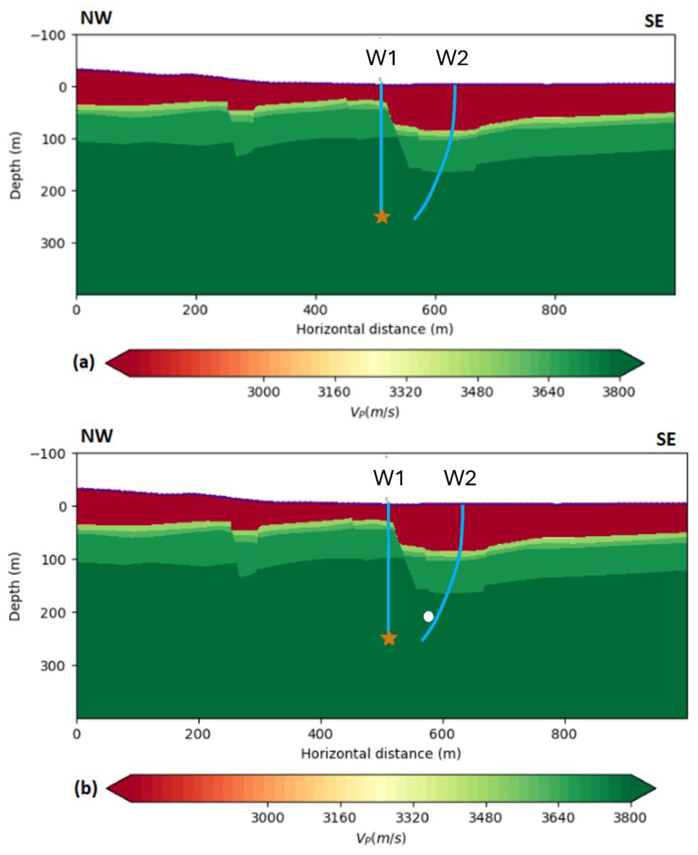
Figure 5.
Pressure components acquired in crosswell configuration after CO₂ injection (a), before injection (b)and as difference between the two (c).
Figure 5.
Pressure components acquired in crosswell configuration after CO₂ injection (a), before injection (b)and as difference between the two (c).
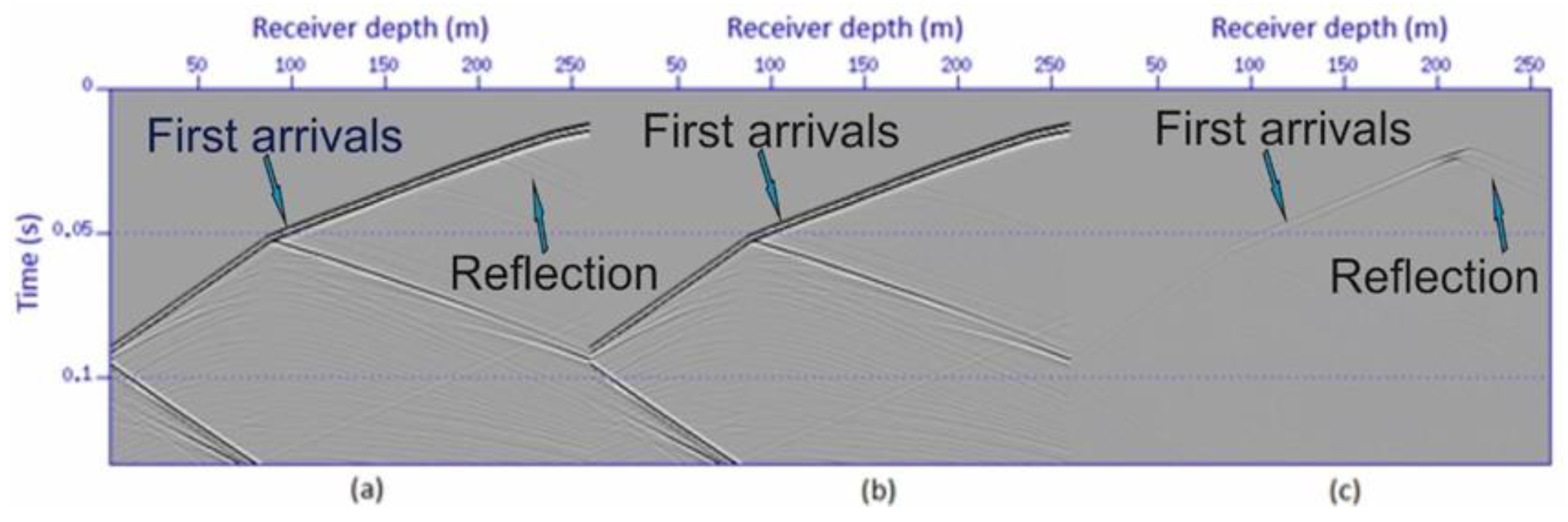
Figure 6.
Vertical particle velocity components acquired in crosswell configuration after CO₂ injection (a), before injection (b)and as difference between the two (c).
Figure 6.
Vertical particle velocity components acquired in crosswell configuration after CO₂ injection (a), before injection (b)and as difference between the two (c).
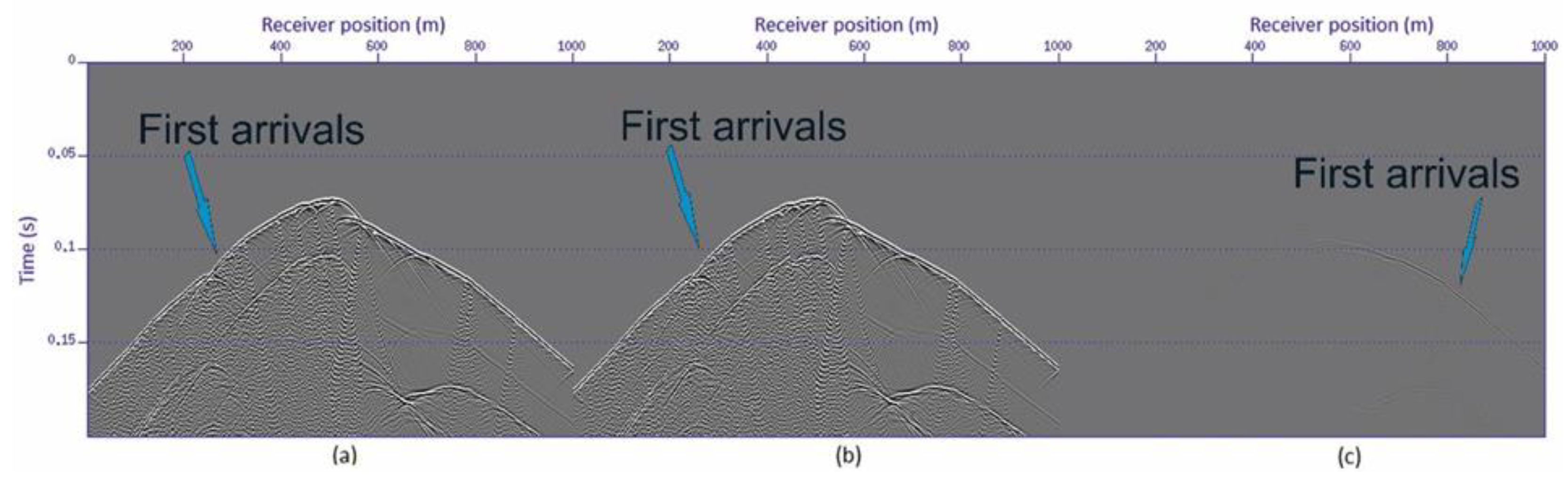
Figure 7.
Map showing the position of the well W1 and the positions of the seismic source for the first near-offset VSP (Shot Point 510) and the second near-offset VSP (Shot Point 530).
Figure 7.
Map showing the position of the well W1 and the positions of the seismic source for the first near-offset VSP (Shot Point 510) and the second near-offset VSP (Shot Point 530).

Figure 8.
Comparison between VSP 510 (above) and VSP 530 (below). (a)Total wavefield of VSP 510 strongly dominated by tube waves and (b) corresponding OWT upgoing wavefield after wavefield separation. The tube waves are attenuated by a F-K filter and the reflections from the subsurface are visible. Data are not bandpass filtered. (c) Total wavefield of VSP 530, the data are less dominated by tube waves, because the source was located farther from the well. and (d) corresponding OWT upgoing wavefield after wavefield separation. The tube waves are attenuated and the reflections from the subsurface are visible. Data are not bandpass filtered.
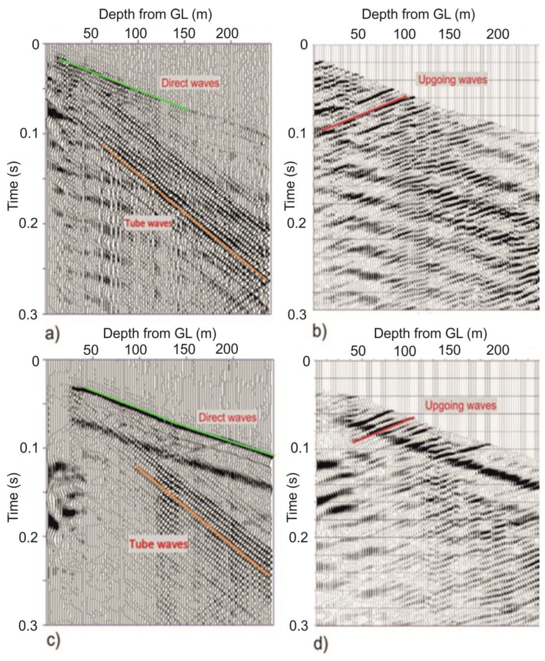
Figure 9.
Interval averaged velocities from VSP 510 (blue solid line). The velocity trends are confirmed by other two VSPs (VSP 480 and VSP 520) from the multioffset survey with hydrophones in W1.
Figure 9.
Interval averaged velocities from VSP 510 (blue solid line). The velocity trends are confirmed by other two VSPs (VSP 480 and VSP 520) from the multioffset survey with hydrophones in W1.
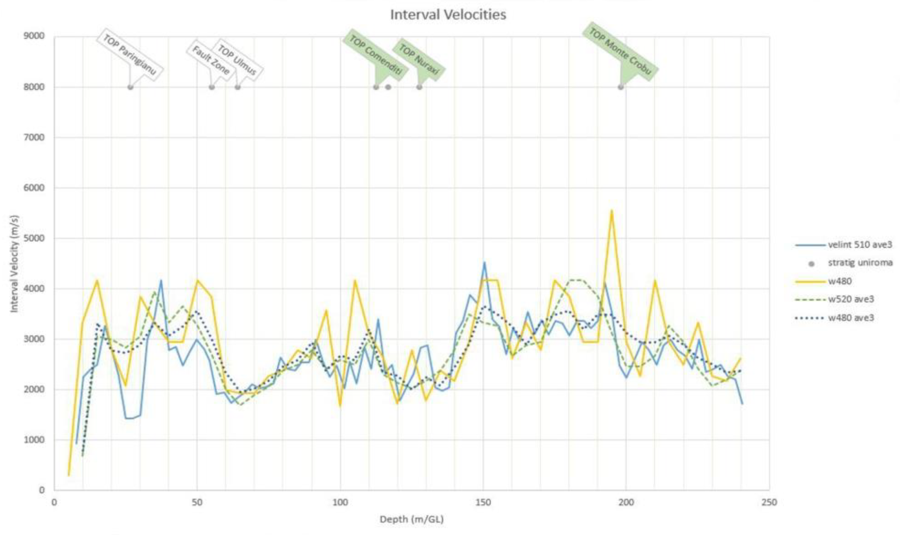
Figure 10.
Composite figure showing how the variations in the interval velocities (up) fit with the reflections in the TWT VSP data (below, on the left). The corridor stack on the right is used for comparison with reflection seismic (Figure 11).
Figure 10.
Composite figure showing how the variations in the interval velocities (up) fit with the reflections in the TWT VSP data (below, on the left). The corridor stack on the right is used for comparison with reflection seismic (Figure 11).
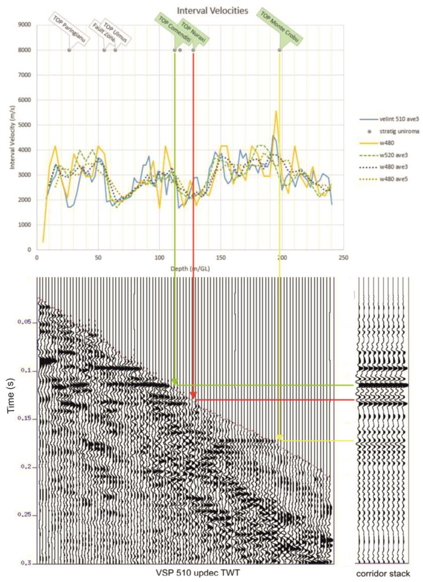
Figure 11.
Stack section of the ine HR1. The corridor stack from near offset data (VSP 510) has been inserted at the position of W1 well on the line after the section was split.
Figure 11.
Stack section of the ine HR1. The corridor stack from near offset data (VSP 510) has been inserted at the position of W1 well on the line after the section was split.
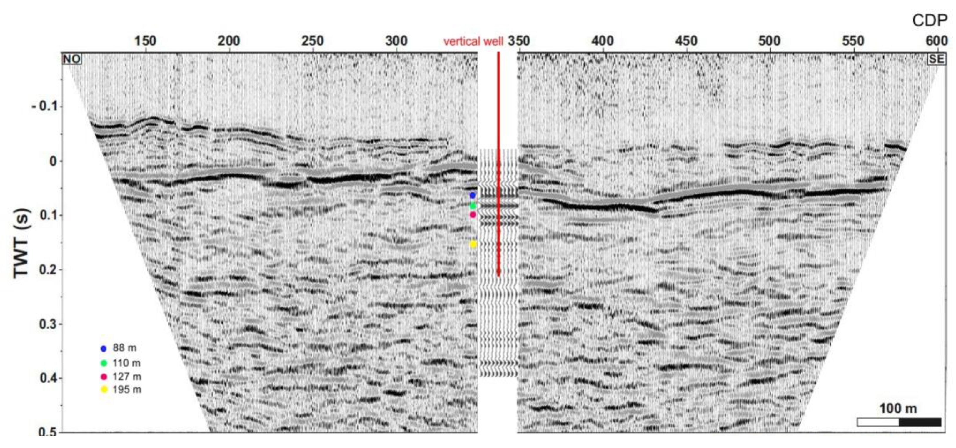
Figure 12.
- Field survey position map with electrodes distribution and well W1 position. All the acquisitions described were acquired in collaboration with Geostudi Astier by using their multi-electrode system SYSCAL Pro 96 resistivimeter for the acquisition.
Figure 12.
- Field survey position map with electrodes distribution and well W1 position. All the acquisitions described were acquired in collaboration with Geostudi Astier by using their multi-electrode system SYSCAL Pro 96 resistivimeter for the acquisition.
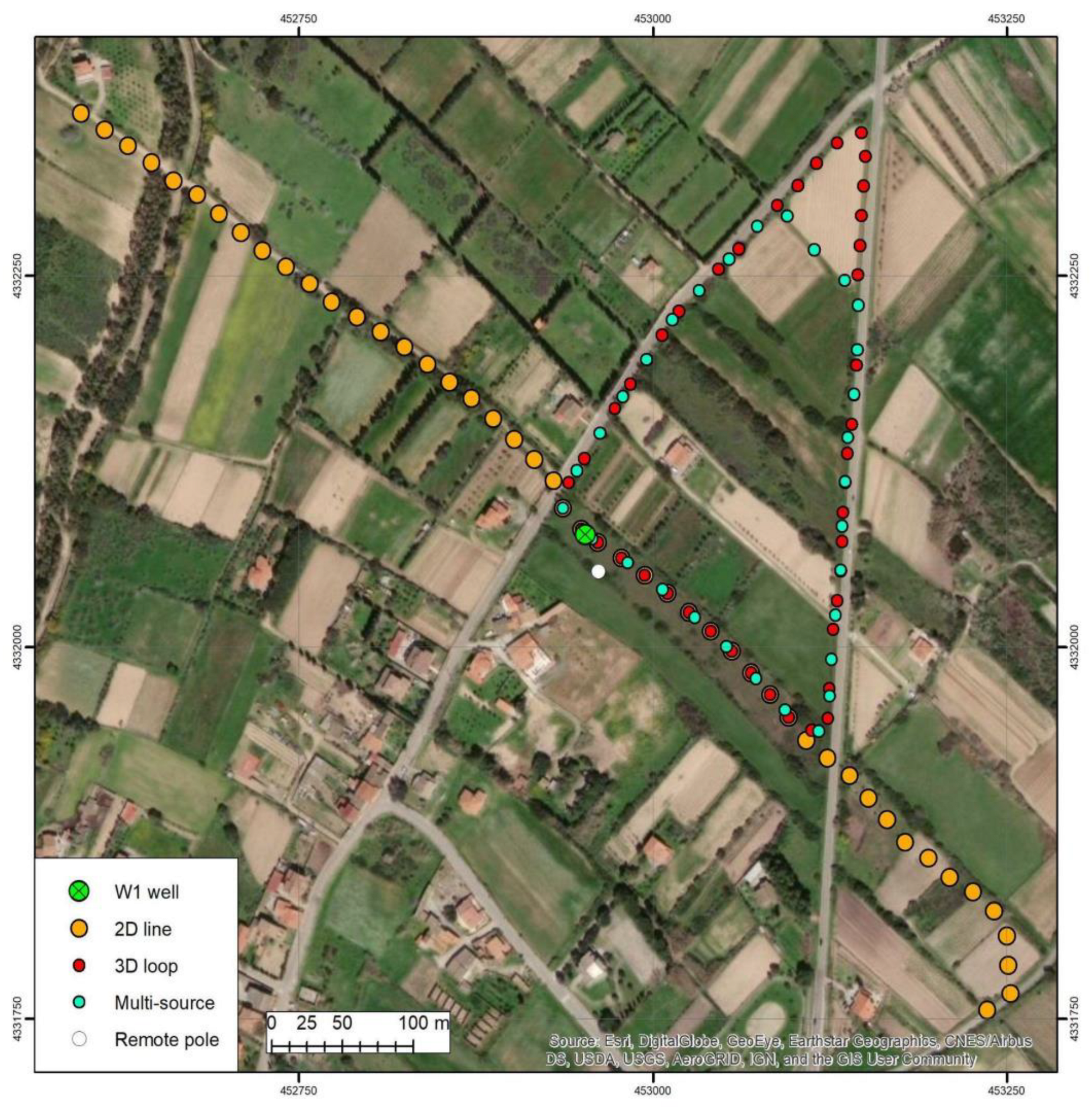
Figure 13.
Joint interpretation between the VSP profile and the 1D resistivity borehole profile.
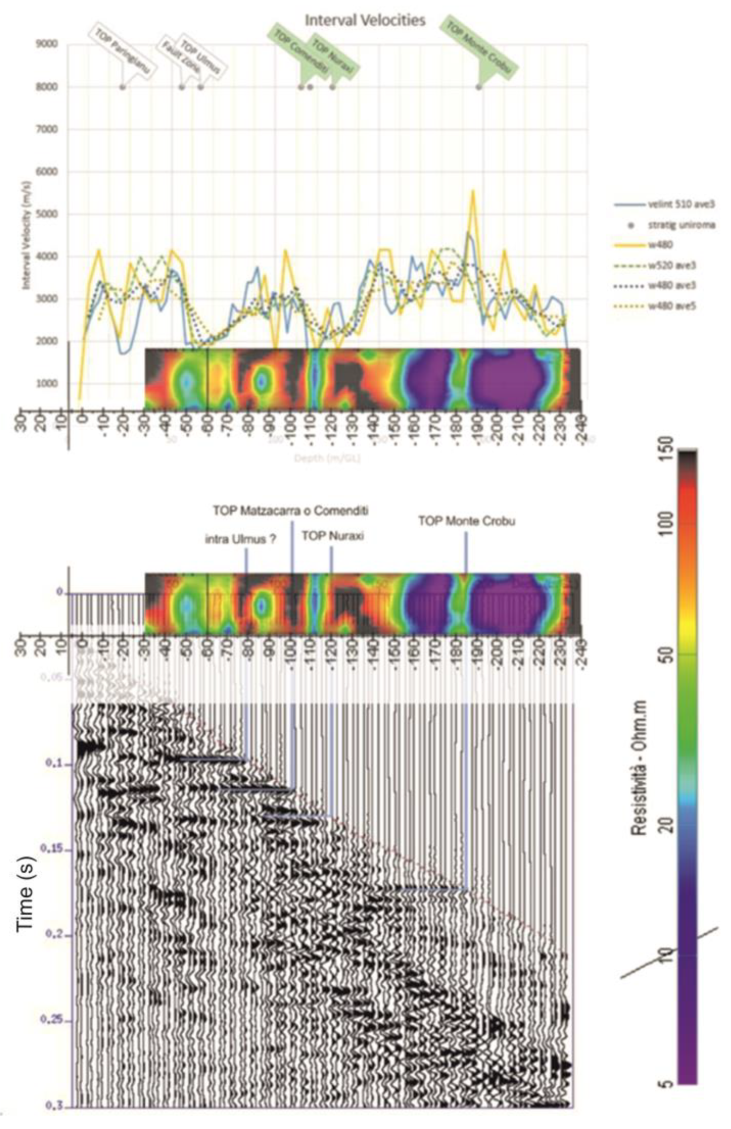
Figure 14.
Wenner – Schlumberger 2D surface resistivity profile superimposed on HR1 interpreted seismic section.
Figure 14.
Wenner – Schlumberger 2D surface resistivity profile superimposed on HR1 interpreted seismic section.
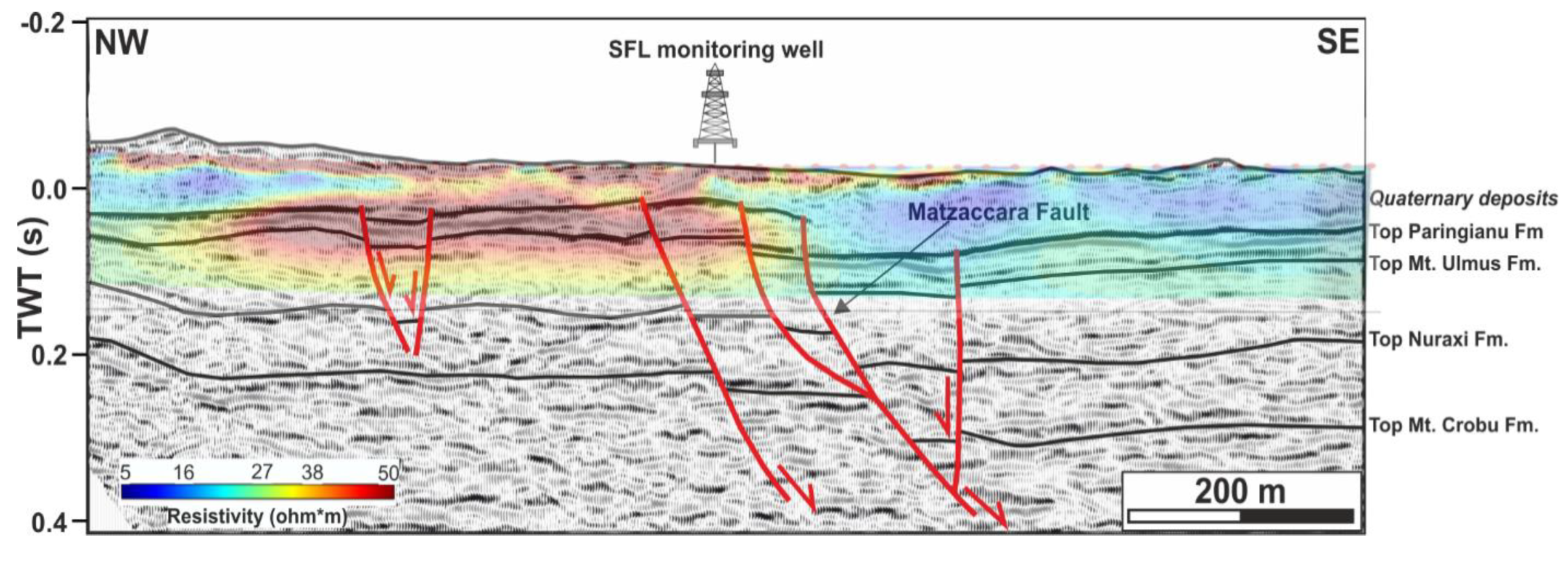
Figure 15.
– Scheme of the actual well configuration of the SFL test bed.
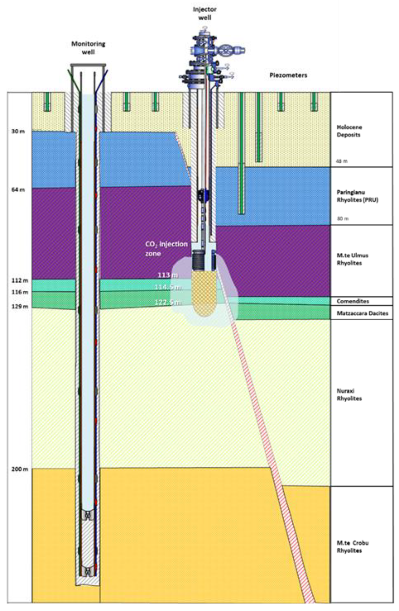

Table 1.
– acquisition parameters for the seismic lines.
| Source: Minivib (upsweep 14 s, 10 – 240 Hz) IVI T-2500 |
| Sensors: geophones 10 Hz (single) |
| Intertraces: 4 m |
| Sampling: 1 ms |
| Time window: 16.4 s |
| intershot: 8 m |
Disclaimer/Publisher’s Note: The statements, opinions and data contained in all publications are solely those of the individual author(s) and contributor(s) and not of MDPI and/or the editor(s). MDPI and/or the editor(s) disclaim responsibility for any injury to people or property resulting from any ideas, methods, instructions or products referred to in the content. |
© 2025 by the authors. Licensee MDPI, Basel, Switzerland. This article is an open access article distributed under the terms and conditions of the Creative Commons Attribution (CC BY) license (http://creativecommons.org/licenses/by/4.0/).
Copyright: This open access article is published under a Creative Commons CC BY 4.0 license, which permit the free download, distribution, and reuse, provided that the author and preprint are cited in any reuse.


