
Submitted:
22 December 2025
Posted:
24 December 2025
You are already at the latest version
Abstract
Injection well placement and rate allocation are among the most decisive factors in determining the efficiency and bankability of CCS projects. However, optimizing these parameters is notoriously complex: even a small number of injection wells leads to a vir-tually infinite set of injection scenarios, while traditional optimization techniques typically require thousands of high-fidelity reservoir simulations. For project developers, this computational burden can stall critical Final Investment Decisions (FID). The proposed approach here addresses this bottleneck by using a Design of Experiments (DoE) framework combined with nonlinear surrogate modeling, which efficiently maps the relationship between injection rates and storage performance, to identify near-optimal solutions with a minimal number of simulations. We show that our method achieves up to 97% of the initially targeted CO2 sequestration with as few as 15 simulations, demonstrating a step-change reduction in time and cost. From a business standpoint, CCS operators can de-risk projects earlier, accelerate FID timelines, and evaluate multiple site configurations in parallel while minimizing computational overhead. Rather than waiting weeks or months for exhaustive optimization, decision-makers can gain timely, reliable insights that directly support capacity commitments, regulatory submissions, and ultimately revenue realization.
Keywords:
CO2 storage
; design of experiments
; CCS optimization
; reservoir simulation
; radial basis function
; D-optimal
1. Introduction
The twenty-first century is witnessing an unprecedented acceleration of climatic change, driven predominantly by the persistent accumulation of anthropogenic carbon dioxide and other greenhouse gases in the atmosphere. Global mean surface temperatures have already risen by approximately 1.1 °C above pre-industrial levels, and this warming is accompanied by profound disruptions: polar ice sheets are retreating at record rates, sea levels are rising faster than at any time in the past two millennia, and extreme weather events, from record-breaking heatwaves to catastrophic floods, have become more frequent and intense [1]. The Intergovernmental Panel on Climate Change (IPCC) projects that, without decisive intervention, global warming could exceed 1.5 °C as early as the 2030s, with cascading impacts on ecosystems, agriculture, human health, and socio-economic stability [2]. These trends underscore that climate change is not a distant threat but an immediate crisis demanding integrated scientific, technological, and societal responses.
Even with aggressive deployment, certain industrial processes will continue to emit substantial CO₂, necessitating complementary technologies capable of immediate, scalable mitigation to sustain economic growth. Among these, Carbon Capture and Storage (CCS) stands out as a transformative solution—bridging the gap between current emission realities and long-term climate goals, while ensuring that industrial growth, economic resilience, and energy security are preserved in the transition toward a sustainable economy [3]. Carbon capture represents the first step in the CCS chain, extracting CO₂ from industrial or power-generation emissions using chemical, physical, or biological processes. Capture technologies are broadly categorized into pre-combustion, post-combustion, and oxy-fuel approaches, each tailored to specific industrial configurations and emission sources [4]. Following capture, CO₂ is transported to storage sites through dedicated pipelines, shipping, or other engineered transport solutions, with robust safety and monitoring protocols to prevent leaks or operational failures [5]. While utilization remains an optional pathway converting CO₂ into chemicals, fuels, or construction materials [6], the storage pillar guarantees permanent removal, forming the cornerstone of climate mitigation in hard-to-abate sectors [3].
Storage involves a coordinated chain of surface and subsurface operations. Surface infrastructure includes wells, pumps, compressors, and monitoring stations that regulate CO₂ injection and ensure operational safety. Subsurface storage relies on carefully selected geological formations where CO₂ is immobilized through a combination of natural forces and mechanisms. Structural and stratigraphic trapping confines CO₂ beneath impermeable rock layers, residual trapping immobilizes it within pore spaces, solubility trapping allows CO₂ to dissolve in formation water, and mineral trapping converts CO₂ into stable carbonate minerals over longer timescales. Effective storage depends on precise placement and control of wells injection rates [7,8], continuous monitoring of well integrity, and rigorous observation of subsurface conditions to prevent leakage and ensure permanent containment, [9,10].
The design and operation of CO₂ storage systems represent one of the most complex engineering challenges within the broader CCS value chain. Unlike capture or transport, the subsurface storage phase is governed by strongly coupled physical, chemical, and operational processes that evolve across multiple spatial and temporal scales. Decisions related to injection design such as placement, sequencing, rate control, and pressure management directly influence the efficiency, safety, and longevity of the storage operation [3].
At the core of any credible and technically sound Storage Development Plan (SDP) lies the injection strategy, or more precisely, the injection schedule a plan that defines how, where, and when CO₂ is injected into the reservoir [11]. The objective is to maximize storage efficiency while satisfying a complex set of multidimensional constraints. These constraints arise from the interplay between subsurface technical factors, operational limitations, and broader economic, commercial, and regulatory conditions. From a technical perspective, pressure buildup within the reservoir must remain below a defined fraction of the fracture pressure to preserve caprock integrity and ensure containment [12]. Simultaneously, plume migration must be carefully managed to prevent CO₂ from escaping the designated storage complex. The geological heterogeneity of the formation variations in porosity, permeability, and capillary entry pressures further complicates this task, rendering deterministic optimization approaches insufficient. Moreover, operational strategies such as brine production or reinjection, which are employed to manage pressure and enhance storage capacity through dissolution mechanisms, add additional degrees of freedom and complexity to the control problem [13]. From an economic standpoint, CO₂ storage optimization involves continuous trade-offs between cost and performance. Higher injection rates or additional wells may accelerate project timelines and increase total storage capacity, but they also raise capital and operating expenditures [14]. Conversely, conservative injection strategies reduce risk yet may underutilize available capacity and delay commercial returns. Balancing these competing objectives requires an integrated optimization framework capable of coupling technical performance metrics with financial, regulatory, and risk-based considerations [11].
Traditional work involves manual heuristic design of the injection schedule however, optimization frameworks those relying on explicit analytical formulations are inadequate for addressing such systems. The objective functions governing CCS operations are inherently non-linear, non-convex, and path-dependent, reflecting the physics of multiphase flow, geomechanics, and chemical interactions in the subsurface [11]. Furthermore, the operational constraints are time-dependent and spatially distributed, rendering closed-form solutions infeasible. As a result, numerical simulation-based optimization becomes indispensable. This approach leverages reservoir simulators to evaluate candidate injection policies, iteratively adjusting control parameters through computational algorithms to converge on optimal or near-optimal solutions.
Meanwhile, simulation-based optimization introduces its own challenges. Each simulation run is computationally expensive [15], and the solution space defined by the combination of well configurations, rates, pressures, and time schedules is vast. Exhaustive search methods are therefore impractical. This motivates this work, where the use of approaches that identify near-optimal strategies—achieving performance close to the true optimum at a fraction of the computational cost—offer a pragmatic alternative. In this study, we propose a method capable of effectively identifying a near-optimal CO₂ storage capacity solution by optimizing wells injection rates with minimal computational effort. The approach is based on two key principles: first, an experimental design of initial points used to train a surrogate model targeted for maximization; second, an iterative refinement of the surrogate model by incorporating the optimal points along with their true simulation responses, continuing until the maximum allowed simulation budget is reached.
In laboratory science, experiments require materials, apparatus, and time, whereas, in computational reservoir engineering, experiments are conducted through numerical simulations, where the primary cost lies in CPU time rather than physical resources [16,17]. Traditional passive data collection in simulations can lead to biased or redundant datasets, reducing the efficiency of model calibration. By contrast, in the first key principle, Design of Experiments (DoE) provides a systematic methodology for varying input factors in an informative and structured manner, ensuring that maximum information is extracted from a limited number of runs [18]. DoE methods can thus be effectively applied to the selection of computational simulations, enabling efficient exploration of the simulation space while minimizing computational cost. In the present framework, DoE is used to select the minimum number of test injection scenarios, still carrying the maximum amount of information on the behavior of the CO2 storage performance function to be optimized. By revealing the nature of the performance function using the DoE sampled injection scenarios, the user can continue with its optimization to identify the optimal one while honoring all physical, mathematical or operational constraints.
Among various DoE methods, D-optimal designs are particularly suitable when simulation costs are high and the design space is large. The D-optimality criterion seeks to maximize the information captured from the design space for a given amount of computational effort, thereby minimizing parameter uncertainty in the surrogate model to follow. For example,[19] developed a D-optimal design framework to build rapid assessment models for CO₂ flooding in high water cut oil reservoirs, using five key reservoir variables and a quadratic regression model to predict recovery factor and net present value. Their study demonstrated that D-optimal experimental design can effectively reduce the number of required simulations while maintaining prediction accuracy, making it a valuable screening tool for CO₂-EOR applications. Similarly, [20] developed a framework for optimizing of reservoir simulation studies that incorporated D-optimal design to efficiently determine optimal well locations under geological uncertainty. Their results showed that D-optimal design helps focus simulation runs on the most informative well configurations, yielding reliable optimization outcomes with far fewer simulations. This approach ensures that each selected simulation contributes maximally to the surrogate model calibration, making D-optimal designs especially effective for screening CO₂ injection strategies in saline aquifers.
Even with carefully chosen DoE originating injection scenarios, the number of simulations may remain insufficient to fully characterize reservoir responses. To address this, surrogate models—simplified mathematical approximations of the true simulation response—are widely employed. Once these surrogates are constructed, optimization techniques can be applied directly to identify promising strategies. For instance, [21] employed a Design of Experiments (DoE) approach combined with Radial Basis Function neural networks (RBF-ANNs) to optimize the Gas–Downhole Water Sink–Assisted Gravity Drainage (GDWS-AGD) process. Their study demonstrated that RBF-based surrogate models can efficiently replace full-physics simulations, accurately capturing the effect of key operational parameters—particularly bottom-hole injection pressure—while markedly reducing computational effort. This highlights the potential of combining DoE with data-driven surrogates to explore complex reservoir behaviors at a fraction of the computational cost.
This work proposes and evaluates a hybrid optimization workflow for CO₂ injection in saline aquifers, designed to rapidly identify near-optimal strategies while minimizing computational demand. The approach is built on five interconnected objectives. First, a D-optimal design of experiments (DoE) is employed to select a minimal but highly informative set of injection scenarios. Second, these scenarios are executed through full-physics reservoir simulations, ensuring that realistic operational constraints such as injection limits, bottom-hole pressure thresholds, and caprock integrity are honored [22]. Third, surrogate models based on polynomial regression or Radial Basis Functions (RBFs) are constructed to approximate the relationship between injection rates and CO₂ storage capacity. Fourth, the surrogate models are optimized using a gradient based optimization algorithm or a Particle Swarm Optimization (PSO) algorithm to efficiently identify near-optimal injection strategies. Finally, the optimized solutions are validated against additional full-physics simulations using the Open Porous Media (OPM) software [23]. Three case studies are presented, demonstrating the efficiency of the proposed method.
By integrating experimental design, simulation, surrogate modeling, and tailored optimization techniques, the proposed workflow enables efficient exploration of the injection strategy design space, balancing computational feasibility with optimization accuracy.
The remainder of this paper is structured as follows. Section 2 reviews the theoretical principles that form the basis of the proposed methodology. Section 3 presents the proposed screening methodology. Section 4 reports the case study, including the static model and operational constraints. Section 5 presents and discusses the results of the three cases. Finally, Section 6 concludes the work.
2. Theoretical Background
This section presents the mathematical foundations that are essential for comprehending the methodology of the present research. It focuses on the principles of the D-optimal experimental design and on the construction of the information matrix. Subsequently, it discusses Polynomial Regression, RBF surrogate modeling and the Particle Swarm Optimization (PSO) algorithm. All those components are involved in various steps of the proposed methodology.
2.1. D-Optimal Design of Experiments Method
For a static process governed by a model of the form , where is the process response and is the vector containing all factors contributing to the response, Design of Experiments (DoE) provides a systematic framework for planning and conducting experiments to efficiently explore the effects of multiple design variables on one or more system responses. Instead of changing one factor at a time, DoE methods vary several factors simultaneously according to a predefined design matrix, allowing the model to estimate main effects, interactions, and nonlinearities with a minimum number of runs [24]. In computational studies, DoE is crucial for selecting the most informative simulation points within the feasible domain, reducing the total computational effort while preserving model accuracy.
Let ΞΝ, of size N × p denotes the full set of all N possible candidate experiments, where each row corresponds to one combination of factors and each column to one of the p design variables. From this set, a subset of n experiments , , is chosen to build the model matrix X of size (n × p), . The information matrix M summarizes how much information the selected experiments provide about the model parameters, defined as:
A higher determinant value of maximizes the volume spanned by the design vectors in p-dimensional factor space. Geometrically, this means the selected experiments cover the factor space as fully and evenly as possible, providing the maximum amount of independent information about the system [25]. Among all possible subsets drawn from ΞΝ, the D-optimal design is the one that maximizes the determinant of the information matrix, described in Equation (2) for a fixed number of runs, n [26].
D-optimal designs are therefore preferred when the total number of feasible experiments is limited or when each model evaluation is computationally expensive, as they provide the maximum information from the smallest possible set of runs [27]. For the purposes of this research, the BoFire (Bayesian Optimization Framework for Real Experiments) library [28] was employed to determine the D-optimal injection scenarios.
2.2. Polynomial Regression
Regression aims to build function forms upon a dataset , where more than one or more independent variables appear in the input and one or more output ones may appear in [29]. In its simplest form, the polynomial regression, we regress one dependent variable on mononomials of a single independent variable. In that case, the model can be expressed as:
where is the degree of the polynomial, , with , are the coefficients of the polynomial and is the fitting error. Equation (3) can be generalized for multiple variables whereas interaction or other non-linear terms between them can also be included, for example . This allows the model to capture not only the individual effect of each variable on the response but also the combined influence of variable pairs or higher-order interactions [30].
In multiple linear regression, the model of one dependent (response) variable on a set of p independent (predictor) variables can be expressed in matrix algebra term by:
The regression surrogate in this study is constructed using the scikit-learn library [31], which fits the model to the training data by minimizing the least-squares error, thereby ensuring an accurate approximation of the response surface.
Once a linear or quadratic polynomial surrogate model (first- and second-order respectively) has been developed, thus the assumption that the response surface is either planar (linear) or convex/concave (quadratic) respectively, the optimal point of the model is then sought [32]. In the case of quadratic model regression, there is a single optimum within the feasible space. This property simplifies the identification of the optimum point to the use of classic gradient-based methods. However, for the problem at hand, there are also equality and inequality constraints, analyzed in the following sections. Those constraints now allow for the optimization of linear surrogate models, or even quadratic ones with the optimum living outside the feasible space. In such cases, the most suitable approach for solving the constrained optimization problem is the Sequential Least Squares Quadratic Programming (SLSQP) algorithm, implemented using the SciPy library [33].
2.3. Radial Basis Function
Radial basis functions (RBFs) are a class of real-valued functions whose values depend on the distance of the operating x from a center point, also known as the radial distance. These basis functions have long been explored in function approximation, machine learning, and pattern recognition tasks [34].
The basic idea in RBFs is to model a function by linearly combining several radially symmetric functions, each centered at a different point in the input space. The output of an RBF network is a linear combination of radial basis functions, weighted by adjustable coefficients. Mathematically, an RBF network with M centers can be represented as:
where are the adjustable weights or coefficients and is the radial basis function, which depends on the distance between the input and the center of each RBF, [35]. The Gaussian function is one of the most widely used RBFs, defined as:
where is the radial distance, and is a parameter value that controls the width or spread of the function [36]. A smaller shape parameter value corresponds to a “flatter” or “wider” basis function. The limit is often referred as the “flat” limit, because corresponds to a constant basis function. In this study, the SciPy library [33]was employed to perform RBF interpolation for constructing the surrogate model.
2.4. Particle Swarm Optimization Algorithm
The Particle Swarm Optimization (PSO) algorithm is a population-based optimization technique inspired by the social behavior of bird flocking and fish schooling. Introduced in 1995, PSO has been extensively applied to a wide range of complex optimization problems in fields such as engineering, machine learning, and computational intelligence.
PSO is initialized with a population of randomly distributed particles, and the optimal solution is sought through iterative updates. Each particle is characterized by two parameters: its velocity and its position at iteration k. In each iteration, the particle updates itself by tracking two ‘extremes’. One extremum is the optimal solution found by the particle itself, which is called the individual extremum and the other extremum is the optimal solution currently found by the entire population, which is called the global extremum [37]. After identifying these two optima, the particle’s velocity and position are updated according to the standard PSO update Equations (A1) and (A2), provided in Appendix A.1.
Through iterative updates of particle velocities and positions, each particle moves toward the global best position that minimizes the objective function, thereby improving the accuracy of the predicted optimum. The optimization procedure terminates when convergence is achieved, defined as a change in the objective function smaller than a specified tolerance [38]. In this study, the PySwarms Python library [39] was employed to implement the PSO framework and perform the optimization of the surrogate model.
3. Screening Methodology
3.1. Problem Definition and DoE Sampling
The injection schedule optimization problem considers injection wells each with its own constant injection rate (Mtpa), over a period of years. The objective is to identify the value for each well which achieve a cumulative CO2 storage target of , where corresponds to the desired total annual injection rate of the field which is screened. Each injection well operates within predefined bounds, expressed by the inequality constraint (8).
The lower limit of (Mtpa) is imposed to avoid the unrealistic scenario of equating the operational power of some well to zero, while the upper limit (Mtpa) corresponds to the typically maximum feasible injection capacity of a single well, mostly depending on the tubing diameter and the CO2 injection temperature [40].
The total injection rate is fixed at the desired value, to serve the emitters need for a guaranteed performance of the field:
Given the equality constraint (9), the problem dimensionality can be reduced to independent variables, with been expressed by:
Applying the bound condition (8) to and substituting Equation (10), results in the inequality constraint Equation (11), which can be rearranged to Equation (12). Finally, isolating leads to in a single inequality constraint, Equation (13), defining its feasible region.
Understanding the feasible design space is essential to correctly interpret the optimization results presented later. In particular, it is important to examine the geometric expression of inequality constraint (13), together with the bound constraints (8), within the - dimensional decision space.
Regarding constraint (8), each inequality restricts the feasible region through two parallel hyperplanes defined by the constants . Since these bounds do not depend on any other variable , they generate axis- aligned, zero-slope constraints that simply limit each to lie within a fixed half-space.
In contrast, inequality (13) introduces a coupling between the variables through the summation term. Geometrically, Equation (13) defines two linear, parallel hyperplanes in the -dimensional space, not aligned with the axes, each involving all variables . More specifically, the left-hand and right-hand sides of Equation (13) impose lower and upper bounds on that vary as functions of the remaining variables. This creates two oblique hyperplanes with non-zero slope, thereby constraining relative to the combined values of the other injection rates.
As a result, the feasible region is no longer a simple hyper-rectangle defined solely by the independent bounds, Equation (8), but a truncated region whose shape depends on how the total injection constraint (9) is distributed among the wells.
To make the formulation of the feasible design space more interpretable, consider a representative example with 3 injection wells, a total field injection rate of 2.0 Mtpa, and operational bounds 0.15 Mtpa and 1.0 Mtpa. From constraint (8), each well rate is bounded between 0.15 and 1.0 Mtpa, whereas Equation (10) reduces the decision space to a two-variable one. The governing relations (8), (10), (13) for this example are therefore:
As discussed earlier, inequality (14) alone restricts the feasible region to a rectangular design space, as illustrated in Figure 1a. Inequality (16) introduces two additional restrictions. To visualize this for the present three-well example, we note that [0.15, 1.0] from Equation (14). The two extreme values of therefore define the two boundary lines of constraint (16), which correspond to the limits of the feasible region in the plane. On the one hand, when 0.15 Mtpa, the bounds for are [0.85, 1.70], but according to Equation (14) it is truncated to [0.85, 1.0]. On the other hand, when 1.0 Mtpa, the bounds for are [0, 0.85], but according to Equation (14) it is truncated to [0.15, 0.85]. The resulting restriction is illustrated in Figure 1b.
After the feasible design space definition, a D-optimal design is generated, constrained to produce only injection schedules within the feasible space, described according to inequalities (8), (12), resulting in a design matrix where each column corresponds to a decision variable and each row represents a sample point, i.e., an injection scenario that needs to be simulated to evaluate the system response, hence the objective function.
The number of simulation points generated, , does not follow a general closed-form formula based on the number of variables and constraints, but rather depends on the available time and computational resources. Indicatively, for the case studies in this work incorporating three injection wells (i.e., two variables) four D-optimal points were generated, whereas for four injection wells (i.e., three variables) nine D-optimal points were produced. If the surrogate model type considered is polynomial (e.g., a quadratic model), then a D-optimal design needs to be generated with a number of points at least equal to the number of coefficients to ensure unique identification of the model parameters, while adding more points can improve precision [29]. In cases where an RBF model is deemed more suitable for capturing the underlying relationship, the goal is to select a number of simulations that adequately cover the feasible space without exceeding the available computational resources. The objective in all cases is to cover the feasible space with as few simulations as possible while still extracting sufficient information. Increasing the number of the D-optimal produced points allows for surrogate models to be fitted in higher accuracy in subsequent steps, while preserving and utilizing the information collected in the first run.
The next step Is to perform reservoir simulations at the designed sampling points. The numerical reservoir flow simulations at each design point, are performed using the Open Porous Media Flow reservoir simulator [23], thereby generating the initial dataset of CO₂ sequestration outcomes by recording the total CO₂ stored at the end of each simulation, the CO2 recycled, the brine produced and the pressure and saturation distribution over the whole reservoir.
Subsequently, the outcomes are evaluated from a reservoir engineering perspective to assess whether the surrogate modeling and optimization techniques that will follow can further improve the maximum point identified, or whether alternative measures might be required to enhance efficiency. For example, by adding an additional injection well to the system.
3.2. Optimization Method
In low-complexity problems, such as systems with one to three injection wells, a simple polynomial surrogate, such as a linear model extended to include interaction effects or a full quadratic model, may be sufficient to accurately represent the D-optimal dataset. In the latter case, the surrogate model is expressed, subject to Equations (8) and (13), as:
where denotes the CO2 total sequestered surrogate’s prediction.
In such cases, a straightforward gradient-based optimization algorithm, such as SLQP can be used to identify the optimal operating point at which CO₂ sequestration is maximized within the feasible space and n is the number of the injection wells.
In contrast, for more complex cases involving four or more injection wells, a Radial Basis Function (RBF) surrogate model with a Gaussian kernel is preferred, as it can capture complex nonlinear interactions among injection rates without incorporating a huge number of the surrogate model parameters. The surrogate model is expressed according to Equations (5), (6) and (7) as:
where is the surrogate prediction of the total CO2 sequestered in Mtn, is the number of simulation points, is the variable operating point, are the RBF centers pointing at the D-optimal solution (training points) and . Conceptually, value determines the range of influence of each Gaussian center: larger values produce narrower Gaussians with more localized effects, while smaller values produce broader Gaussians affecting a wider region.
For the initial RBF surrogate, the γ value is selected randomly between 0.1 and 1.0. This approach aims to create a smoothed surrogate in which the influence of individual points is more evenly distributed, rather than being dominated by the maximum point. The choice of the initial random γ value does not yet affect the optimization result, as it will be adjusted in the subsequent optimization step.
After constructing the RBF surrogate from the D-optimal design points, a primary Particle Swarm Optimization (PSO) algorithm is employed to identify the operating point that maximizes CO₂ sequestration, described in Equation (20) subject to the constraint (8), by minimizing , Equation (21). Note that can be extended to consider any additional effects, such as plume expansion, contribution of different storage mechanisms, leakage penalty or cash-flow related terms.
Followingly, a reservoir simulation of the resulted is performed. Τhe actual CO₂ sequestered value (, as obtained by another simulation run, is recorded and its absolute prediction error is calculated by the Equation (22) and also documented.
The next step is to employ a secondary PSO algorithm to determine the γ* parameter value that minimizes the surrogate’s absolute prediction error at by minimizing , as described in Equation (23). This γ parameter value optimization step ensures that the surrogate is optimally fitted in the region where the best solution is expected to lie, thereby improving local accuracy and the reliability of the subsequent optimization.
The procedure subsequently continues by incorporating the identified into the surrogate’s training set and refitting the RBF surrogate model with the updated dataset and the optimized γ* value. Followingly, the primary PSO algorithm is re-executed to search for the new optimal solution that minimizes based on the updated surrogate. The entire procedure is repeated iteratively by running one additional simulation per iteration, until either three consecutive optimal solutions are obtained and found equal up to some threshold, or until a total of 15 sampling points has been reached. All supporting details regarding the PSOs specifications, are provided in Table A1 and Table A2, Appendix A.2.
4. Case Studies
For this research, a detailed aquifer case study is developed to evaluate the proposed CO₂ storage optimization strategies. The reservoir static model has been employed in previous studies, [7,41], focusing on optimal well placement and flow rates allocation, leveraging Bayesian optimization frameworks. By employing this established static model, where the well placement has already been optimized, the influence of well location on the results is eliminated. This ensures that the present study focuses solely on evaluating the impact of operational and economic factors, such as injection strategies and CO₂ storage performance, without any interference from well placement variability.
The corner-point geometry reservoir grid comprises of 120 × 163 × 4 cells (X, Y, Z), totaling 78,240 cells, of which 9,212 are active. Inactive cells define non-flow zones and are excluded from flow computations. The aquifer exhibits an inclined structural profile with a steep anticlinal crest, which acts as a trap for buoyant CO₂, illustrated in Figure 2.
The depth of the reservoir, shown in Figure 2, ranges from 9,311 ft at the crest to 10,850 ft at the deepest point. A hydrostatic pressure–depth gradient of 0.465 psi/ft [42] was used in the model, resulting in a normal initial reservoir pressure between approximately 4,330 psi at the crest and 5,045 psi at the deepest point, with an average pressure of about 4,700 psi.
For the temperature–depth relationship, a geothermal gradient of 0.0142 °F/ft [43] was applied. The temperature at depth (ft) is calculated using Equation (24):
where = 77 °F is the surface temperature and is the geothermal gradient. Based on this, the crest temperature is approximately 209 °F, while at the deepest point the temperature is about 231 °F, giving an average reservoir temperature of roughly 219 °F.
The reservoir is structurally simple and sealed by impermeable shale, with a bulk volume of 240 MMMft³, initial water in place of 1.7 MMMSTB, salinity of ~65,000 ppm. Permeability is anisotropic and heterogeneous: horizontal permeability ( = ) has P90 = 91 mD, P50 = 272 mD, P10 = 572 mD, while vertical permeability () is one order of magnitude lower, favoring lateral flow. The spatial distribution of permeability X is provided in Figure 3. Porosity is uniform at 0.25, indicating stable storage capacity. The CO₂–brine (water) relative permeabilities are also given in Table 1, Appendix B.1 [15], and their plot is presented in Figure 4.
Three vertical injectors I1, I2, I3 are placed in the downdip reservoir region to promote controlled upward CO₂ migration, whereas eight brine producers P1 to P8 are positioned to manage reservoir pressure and direct the plume movement, Figure 5. Notably, P6 acts as a pressure sink along the plume path, and P4 ensures uniform migration despite buoyancy-driven asymmetry. The specific placement of each well is also provided in Table B2, Appendix B.1, and the operational specifications of all wells are summarized in Table 1 where, to facilitate notation, the wells are distinguished according to their operational role into producers and injectors.
The storage process is scheduled for 40 years. Field-level constraints limit brine production below 80 Mstb/day based on the brine treatment facilities capacity, while individual production wells are allowed a brine production of 60 Mstb/day as dictated by the wellbore capacity. CO2 field recycling of 6 MMscf/day at maximum, CO2 recycling of 4 MMscf/day at maximum per well, bottom-hole pressure (BHP) floored at 3,000 psi for producers and capped at 9,000 psi for injectors, are also constraining the problem solution.
Bottom-hole pressure constraints have different purposes for producers and injectors. On the one hand, for the injectors, the BHP constraint is applied to ensure that the pressure does not exceed the upper fracture limit of the caprock, thereby preventing the activation of potential CO₂ leakage pathways [3]. On the other hand, the BHP constraint for producers is imposed to ensure that reservoir depressurization occurs in a controlled and gradual manner [44]. In this study, a value of 3,000 psi is adopted for producers, following previous work [7] based on the BHP required to lift the produced brine at surface, without explicitly assessing its influence on the overall problem solution.
It is noted that when a constraint is activated at some well, the simulator reduces the CO2 injection rate or the brine production rate to honor the constraint [45]. For instance, when an injection well reaches its BHP limit of 9,000 psi, the simulator reduces the CO₂ injection rate to maintain the well pressure at its upper bound (9,000 psi).
Initially, the field CO₂ injection target is set at 2 Mtpa, which corresponds to approximately 107.4 MMscf/day, aiming at a total cumulative injection of 1.57 Tscf (equivalent to 80 Mtn) over the project’s lifetime. The term Mtn denotes million ( tonnes and Mtpa million tonnes per annum, while Mscf stands for thousand ( surface cubic feet, MMscf = scf. All simulations were run using the CO₂ storage module in Open Porous Media Flow [22].
It is important to highlight that the only way to predict, identify and guide the system’s behavior during injection stages is by imposing operational constraints on the operating wells, as these wells provide the only direct measurements available under real field conditions [46]. For this reason, it is essential to carefully define the operating constraints of the wells.
5. Results & Discussion
5.1. Case 1: Total Field CO2 Sequestration Target 80 Mtn with Three Injection Wells
The injection schedule optimization problem involves three wells with constant injection rates , , (Mtpa) over a period of 40 years. With an operations management decision of achieving a design total target of 2.0 Mtpa × 40 years= 80 Mtn, the total injection rate T is fixed at 2.0 Mtpa. The problem dimensionality reduces to two independent variables, as described by Equation (26) and subject to the condition (25), in accordance with Section 3.1.
The feasible space for the two variables under the constraint is illustrated in Figure 6. A D-optimal experimental design was conducted to cover this space as effectively as possible by only using a user specified low number of points. When using three sample points, the algorithm selects points 1, 2, and 3, illustrated in Figure 6a, simply capturing the extremes of the feasible space. To gain additional insight into the system’s behavior in other regions of the design space, the D-optimal design algorithm was further asked to generate a fourth distinct combination of the well injection rates , , indicated by point 4 in Figure 6a. The feasible space restricted by the problem’s constraints is demonstrated by the light green area
After generating the DoE design schedules, simulations were performed using the Open Porous Media (OPM) Flow reservoir simulator to collect the reservoir response, i.e., pressure build up, CO2 sequestered, CO2 recycled and brine production. The desired CO₂ sequestration capacity was verified for all sampling points, yielding 80 Mtn in 40 years of operation as seen in Table 2.
The fact that the desired target storage of 80 Mtn has been directly achieved, even before any optimization takes place, demonstrates that additional sequestration capacity can be realized; for example, targeting an injection rate of 2.5 Mtpa over 40 years, which would result in a total sequestration of 100 Mtn, might be feasible.
5.2. Case 2: Total Field CO2 Sequestration Target 100 Mtn with Three Injection Wells
In this case, the objective is to achieve a maximum total target of
2.5 Mtpa × 40 years = 100 Mtn, hence the field injection rate T is set at 2.5 Mtpa. Consistent with the procedure applied in Section 3.1, the feasible design space is now constrained by Equation (27), subject to condition (25).
The feasible space for the two variables, along with the four D-optimal points generated, is illustrated in Figure 6b. Note that the feasible space has been remarkably reduced due to the increased storage request.
The simulation results recorded at the end of the reservoir simulation of each D-optimal design point, where is CO2 sequestration in Mtn, are shown in Table 3. The highest sequestration capacity was obtained at point , ), which lies to the boundary of the feasible space, yielding 93.3 Mtn of CO₂, corresponding to 93.3% of the initial 100 Mtn target. It should be noted that the achieved sequestration capacity is influenced by the constraints imposed on the system. Specifically, under the bottom-hole pressure (BHP) constraints, the injectors were unable to inject as much CO₂ as desired, since the system automatically adjusts injection rates to comply with the prescribed pressure limits. In other words, the simulator is instructed to maintain a constant rate all over the full injection period, however the rate achieved subject to the operational constraints proved to be lower than the desired one.
Although the D-optimal design alone proved sufficient to identify a high-quality solution, fitting a surrogate model based on these points and the optimization process using a gradient-based algorithm was still pursued. This would validate the surrogate model prediction accuracy and investigate whether an alternative configuration within the feasible space might yield a superior outcome. By fitting a second-order surrogate model with only interaction effects to the D-optimal points, Equation (28) is obtained, where .
Figure 7 and Figure 8 effectively illustrate the relationship between the prediction values and the problem’s input variables . It also shows that, outside the feasible space, even higher predicted solutions could be obtained by the surrogate model. However, these solutions are not considered not only for lying outside the feasible space, that is they violate the per-well operating bounds of 0.15 Mtpa (lower) and 1 Mtpa (upper), subject to the condition (25). From a fitting point of view, such values are produced by pure extrapolation, hence they are fully uncontrollable.
The optimization of the surrogate model resulted in a optimal point with I1 and I2 (corresponding to I3), that is the best already obtained D-optimal result ( indicating that the surrogate model optimization did not achieve any better than the DoE sampled points. This is attributed to the fact that the surrogate model proved to be monotonic within the feasible space with no internal optimal. Nevertheless, the predicted CO₂ sequestration at three additional random points within the feasible space was compared against validation simulations. The results (Table D1, Appendix D.1) confirm the high accuracy of the selected surrogate and support the conclusion that no scenario surpasses the initial D-optimal maximum.
Figure 9 demonstrates the CO₂ plume expansion at four distinct time steps. The simulation starts with all cells exhibiting 100% water saturation (not shown). At t = 10 years, injection wells I₁ and I₃ have the most pronounced effect on CO₂ migration, as initially planned. At t = 20 years, the three CO₂ plumes merge into a single plume, which at t = 30 years begins to pass over the anticline. Finally, in t = 40 years, the plume has fully traversed the anticline, with a total CO₂ sequestration of 93.3 Mtn.
Figure 10 illustrates the spatial distribution of reservoir pressure at the end of the injection period. The most critical zone is the caprock, where maintaining pressures below the fracture threshold is essential to ensure mechanical integrity during CO₂ injection. The spatial distribution indicates that the maximum reservoir pressure reaches approximately 9,000 psi, remaining safely below the caprock’s fracture-pressure limit and thereby preventing overpressurization. Figure 11 also shows that the initial average reservoir pressure of 4,700 psi decreases during the first five years and then begins to rise, reaching approximately 8,100 psi by the end of the project.
Note that corresponds to the intended injection schedule identified by the optimizer. When the simulator implements that, it is possible the amount of CO2 actually arriving bottom hole might be less than the optimal due to potential activation of the injectors BHP constraint (9,000 psi). In this case, the injection process begins at a maximum rate of 134.5 MMscf/day (2.5 Mtpa), which is sustained for 34 years. After this period, a decline occurs for the remaining 6 years of the injection period, eventually arriving at 83 MMscf/day (1.54 Mtpa). On the other hand, the field’s maximum water production rate of 77,000 stb/day is never reached. Undesired CO₂ production begins after approximately 5 years of operation and gradually increasing until a peak of 6.0 MMscf/day (0.11 Mtpa), reached after 22 years. The CO2 field injection and production rates over time are demonstrated in Figure 12.
The injection wells performance is further illustrated in Figure 13 and Figure 14, which show the bottom-hole pressure of each well and their injection rates over time respectively. The initial wells’ bottomhole pressure (BHP) appear significantly higher than the pressure at the deepest point of the reservoir. This is due to the localized pressure buildup that develops at the very beginning of CO₂ injection. Moreover, each well shows a different starting BHP, which is explained by two factors: the differences in well depth and the fact that each well begins injecting at a different initial injection rate.
I3 (green) initially maintains a constant injection rate of 53.7 MMscf/day (1.0 Mtpa) for the first 34 years. Subsequently, bottom-hole pressure limit is reached, resulting in a declining injection rate for the remaining 6 years. I1 (blue) maintains a steady injection rate of 53.7 MMscf/day (1.0 Mtpa) for 35 years until the bottom-hole pressure constraint is activated. After that its rate declines over the final 5 years. I2 (purple) consistently injects 27.1 MMscf/day (0.50 Mtpa) during the whole operation since no bottom-hole pressure reached.
5.3. Case 3: Total Field CO2 Sequestration Target 100 Mtn with Four Injection Wells
Although, the procedure in Case 2 proved sufficient to identify a near-optimal solution, achieving 93.3% of the targeted sequestration capacity, the full goal was not reached, due to the injector’s BHP constraints. To address this shortfall, the potential benefits of adding an additional injection well could be investigated, as this is expected to improve efficiency by enhancing the feasible space dimensionality, thus allowing greater sequestration capacity.
By keeping the injection target at 100 Mtn while introducing one more injector, I4, bounded by the same minimum and maximum rate constraints as the other wells, the design space is expanded. Τhe location of the new introduced well I4 is illustrated in Figure 18. Nine D-optimal sample points were selected within this enhanced 3D feasible space. The sampling points and their distribution are illustrated in Table 4 and in Figure 15 respectively. The operational constraint for the three variables problem in this four-well configuration was defined with Equation (29) subject to the condition (25).
Simulations were performed using the Open Porous Media (OPM) Flow reservoir simulator, producing a dataset of observations. Table 4 illustrates the simulation results for these D-optimal points, where the amount of CO₂ sequestered is expressed in Mtn. The highest sequestration capacity was obtained at the sixth D-optimal simulation point (I₁ = 0.15, I₂ = 1.0, I3 = 0.9, I4 = 0.45), yielding a total of 96.1 Mtn of CO₂, hence demonstrating that the additional injection well provides a better, still not optimal solution.
By fitting a second-order surrogate model keeping only the interaction effects to the D-optimal points the resulting fitted model is described in Equation (30), where are in Mtpa, [0, 0.15].
The gradient-based optimization predicted a maximum of approximately 120 Mtn at the point (corresponding to ), which is physically unrealistic given that the true maximum possible CO₂ sequestration is 100 Mtn (40 years injection of 2.5 Mtpa). This overestimation arises because the second-order model limited to the interaction effects only, is a simplistic approximation of the true response surface, highlighting the limitations of the surrogate model form when extrapolating beyond the sampled domain.
To improve the surrogate model, a full quadratic model was fitted after incorporating the 10th D-optimal design point 0.78, 0.57, 1.0, and running the corresponding simulation, which yielded 91.3 Mtn of sequestered CO₂. The resulting quadratic model is given by:
Optimizing this quadratic model with a simple gradient-based algorithm thanks to its constant curvature, the predicted optimum occurs at with a maximum predicted CO₂ of 111.55 Mtn, which again is physically unrealistic, though less exaggerated than in the previous attempt. This demonstrates that, while quadratic models improve the fit within the sampled space, they still may overestimate values outside the convex hull of the design points, emphasizing the need for caution required when the built surrogate models are extrapolated.
Considering that a third-order model would require 20 design points, and in order to avoid exceeding computational costs—since the method aims to screen near-optimal solutions with as few simulations as possible—we adopt an alternative approach, described in Section 3.2. Specifically, the D-optimal points are first used to fit an RBF surrogate model equipped with gaussian kernel, which is then optimized using PSO. This strategy is designed to limit the total number of simulations to a maximum of 15, while still effectively exploring the feasible space to identify high-quality solutions.
When an RBF model is involved additional simulation runs can also be used to optimize the surrogate model’s hyperparameter γ. Indeed, the RBF surrogate based on the nine D-optimal sampling points dataset was fitted, using a randomly selected shape parameter value of 0.85. The PSO algorithm was then ran and identified the new solution, which was subsequently simulated using OPM Flow, yielding a CO₂ sequestration of 96.8 Mtn. Next, PSO algorithm was employed again, this time to determine the γ value that minimizes the absolute prediction error of (Mtn) at the solution, resulting in γ value equal to 0.73, point 10 in Table 5. The solution, along with its response, was then added to the surrogate’s training set, and the RBF was refitted. The results at each iteration of this process are presented in Table 5. Finally, after three consecutive iterations, it was concluded that the identified point (0.21, 0.93, 0.96, 0.40) maximizes the sequestration capacity at 97.4 Mtn, its placement is plotted in Figure 15. This dual approach kept producing new sampling points, on top of the first D-optimal based ones, to improve the local accuracy of the surrogate model, hence its optimum well rates point.
To assess the predictive reliability and generalization capability of the final optimized surrogate, an independent validation was performed. The performance of the final RBF surrogate, with its optimized γ parameter, γ*, was validated using five additional random testing samples within the feasible design space. The analytical results (Table C2, Appendix C.2) indicate that the absolute total error across the five testing points is 3%, with a standard deviation of 0.313, confirming the high predictive accuracy of the RBF surrogate with gaussian kernel. This validation demonstrates the effectiveness of the proposed screening methodology and its applicability to optimization problems of similar dimensionality.
Furthermore, the effect of the optimized γ parameter was assessed to evaluate how the final model would perform without its optimization, using a randomly chosen value instead. As described in Section 3.2, the γ parameter was optimized to ensure that the RBF surrogate performs optimally, particularly in the region surrounding the maximum solution point. In the proposed methodology, the γ parameter was randomly initialized at 0.85, and the optimizer converged to γ* = 4.2, following the path shown in Figure 16.
To highlight the impact of γ optimization, the fifteen-point RBF surrogate was evaluated at the same five testing points used for overall surrogate accuracy, considering eight γ values: 0.77, 2.4, 3.3, 4.2, 5, 10, 50, and 100. The results (Table C3, Appendix C.2) show that low γ values (<2) lead to a high total absolute error (~8%), intermediate values around 4 minimize the error (~3.2%), and high values (>10) cause a slight increase. Figure 17 illustrates these trends, including a zoomed-in view around the minimum absolute error. These results validate that the proposed algorithm reliably determines γ*, achieving optimal surrogate performance.
The predicted CO₂ sequestration at the optimum corresponds to 97.4 Mtn, representing an additional 4.1 Mtn compared to the three-well model and bridging the performance of the optimized injection schedule further close to the desired 100 Mtn target. This result demonstrates that adding an additional operating well can efficiently achieve a better outcome, since the capacity increased. Furthermore, it indicates that the system may not be able to exceed the upper bound of 100 Mtn under the current operational constraints. This proposed approach not only identifies a physically consistent solution—since, in contrast to previous polynomial surrogates (second order), it yielded a value below the 100 Mtn —but also provides an improved performance relative to the original three-well configuration.
The detailed simulation results corresponding to the maximum response identified from the optimizer are also presented. Similarly to the results in Case 2, Figure 18 illustrates the CO₂ plume at four distinct time steps. At t = 10 years, injection wells I₂ and I₃ exert the strongest influence on CO₂ migration, consistent with the initial design. At t = 20 years, the I2, I3, I4 CO₂ plumes have merged into a single stream that has started to migrate across the anticline. From t = 30 years to t = 40 years, the plume has fully traversed the anticline, with a total CO₂ sequestration of 1.91 Tscf, approximately 97.4 Mtn.
Figure 19 demonstrates the spatial distribution of reservoir pressure at the end of the injection period. It is noted the criticality to ensure that the pressure remains below the caprock fracture threshold while the reservoir is being pressurized by CO₂ injection. Furthermore Figure 20, indicate that the maximum reservoir pressure reaches 9,000 psi, remaining safely below the caprock fracture pressure limit and thus preventing overpressurization.
The optimal scenario field CO₂ injection and recycling rates are demonstrated in Figure 21. The injection process begins at a maximum rate of 134.5 MMscf/day (2.5 Mtpa), which is sustained for 38 years, that is almost all the duration of the project. A decline is observed only during the last 2 years of the injection period, eventually arriving at 113.8 MMscf/day (2.12 Mtpa), which still corresponds to 85% of the design rate on the very last day. On the other hand, the field’s maximum water production rate of 77 Mstb/day is never encountered. Undesired CO₂ production due to recycling through the brine producers begins after approximately 18 years of operation gradually increasing to a peak of 6.0 MMscf/day (0.11 Mtpa), reached at t = 27 years, and remains constant until the end of the project.
The individual well performance at the optimized schedule is further illustrated in Figure 22 and Figure 23, which show the bottom-hole pressures of each well with and their injection rates over time. I4 shows a lower starting BHP compared to the other wells. This is explained by the shallower depth of its perforations—being located at a higher structural position.
I3 (green) maintains a steady injection rate of 51.5 MMscf/day (0.96 Mtpa) for 38 years. Subsequently, the bottom-hole pressure limit is reached, resulting in a declining injection rate for the last 2 year. I2 (purple area) maintains a steady injection rate of 49.9 MMscf/day (0.93 Mtpa) for 39 years until the bottom-hole pressure constraint is reached. I4 (orange) and I1 (blue) consistently inject 21.5 MMscf/day (0.40 Mtpa) and 11.2 MMscf/day (0.21 Mtpa) respectively, throughout the entire 40-year period with no decline. The well rate profiles are in alignment to the pressure profiles which confirm that I3 gets BHP constrained at t = 38 years, while I4 does so at t = 39 years. I1 and I2 are not limited, hence they maintain their design rate, as dictated by , until the completion of the project.
5.4. Discussion
Table 6 summarizes the outcomes of the various CO₂ injection scenarios examined. Each case differs in the number of injection wells and the targeted sequestration amount. The achieved CO₂ sequestration closely matches the targets, demonstrating the effectiveness of the designed injection strategies. Table 6 also lists the number of D-optimal design points and the total simulations required for each scenario, highlighting the efficiency of the experimental design approach.
The results indicate that, under the specified operational constraints, the system captures significantly more CO₂ than Case 1’s target of 80 Mtn in Case 2, despite having the same number of wells. In Case 3, although the proposed methodology successfully captures system relationships and provides a physically consistent solution, the addition of a fourth well yields only a marginal increase in sequestration, 4.1 Mtn, compared to Case 2 with three wells. From a reservoir engineering perspective, this solution is less attractive economically, as the additional well increases both CAPEX and OPEX disproportionately to the small gain in storage.
Despite the diminishing returns observed when adding more wells, the methodology itself proves robust and effective in capturing the system’s behavior and identifying optimal injection configurations making it a reliable tool for decision-making. Beyond maximizing CO₂ storage, the framework can be readily extended to more complex, multi-objective optimization problems, such as maximizing net present value (NPV) or balancing economic efficiency with storage performance. This flexibility demonstrates that the proposed approach is not only effective for single-objective optimization but also capable of supporting more comprehensive reservoir management strategies.
For future extensions, the methodology can be adapted to incorporate time-dependent injection strategies by splitting the project period into multiple time steps and optimizing injection controls for each step [11]. This approach allows more dynamic management of CO₂ injection, potentially improving performance or balancing economic and operational objectives over time. The same surrogate-based framework is likely suitable for this extension; however, increasing the number of time steps also increases the problem’s dimensionality, creating a trade-off between computational cost and surrogate accuracy. Careful experimental design and potentially adaptive surrogate updating would be needed to maintain efficiency while preserving reliable predictions.
Beyond CO₂ storage, the methodology provides a practical and scalable tool for real-world dynamic subsurface management [47] and can be extended to other applications, including open reservoir CO₂ storage systems [48], geothermal production [49] and hydrogen storage [50]. The effect of CO₂-stream impurities on storage mechanisms can also be investigated, further broadening the applicability and robustness of the approach [51].
6. Conclusions
The proposed methodology addresses this need by integrating experimental design, surrogate modeling, and intelligent optimization to efficiently identify near-optimal injection strategies under realistic physical, operational, and commercial constraints. Rather than relying on computationally expensive exhaustive reservoir simulations, the approach minimizes simulation cost while preserving decision quality, making it particularly attractive for portfolio screening, feasibility studies, and scenario evaluation under contractual injection commitments.
Specifically, the methodology implements an integrated optimization framework that combines D-optimal experimental design, radial basis function (RBF) surrogate modeling, and particle swarm optimization (PSO). This framework is specifically tailored to support early-stage decision making and operational planning, where rapid assessment of feasible injection strategies is critical for both technical and commercial viability.
From a commercial and strategic perspective, large-scale CO₂ storage (CCS) projects must balance three competing objectives: maximizing contracted CO₂ intake, minimizing operational and computational costs, and reducing technical and financial risk over multi-decadal project lifetimes. Injection strategies directly affect a project’s ability to honor long-term CO₂ offtake agreements with emitters, ensure stable revenue streams, and protect capital investments in wells and surface infrastructure. Consequently, decision-makers require optimization tools that are not only technically robust, but also fast, interpretable, and suitable for early-stage screening and operational planning.
Author Contributions
Conceptualization, E.T.D and V.G.; methodology, E.T.D; software, E.T.D. and S.P.F.; validation, E.T.D., V.G. and S.P.F.; formal analysis, E.T.D. and V.G.; investigation, E.T.D.; data curation E.T.D.; writing- original draft preparation, E.T.D. and I.I.; writing- review and editing, V.G. and S.B.; visualization, E.T.D.; supervision V.G.; All authors have read and agreed to the published version of the manuscript.
Funding
This research received no external funding.
Appendix A
Appendix A.1.
In these expressions, denotes the inertia weight, which balances global and local search abilities. A larger value of ω enhances global exploration, while a smaller value strengthens local exploitation. The parameters and , are the acceleration coefficients, typically both are assigned values between 0 and 2. Moreover, the random variables and are uniformly distributed in the interval [38].
Appendix A.2.

Table A1.
Subordinator PSO algorithm specifications, for identifying optimal parameters.
| Acceleration coefficients & |
γ value searching bounds |
Particle swarm size | Maximum iterations |
| 0.5 | (0.1, 100) | 100 | 100 |
Table A2.
Primary PSO algorithm specifications, for identifying optimal .
| Acceleration Coefficients & |
well rates searching bounds |
Particle swarm size | Maximum iterations |
| 0.5 | (0.15, 1.0) | 100 | 100 |
Appendix B
Appendix Β.1.
Brine relative permeability is 1.0 at zero CO₂ saturation and decreases sharply as CO₂ saturation rises, while CO₂ relative permeability starts near zero and gradually increases, reflecting typical two-phase flow in water-wet reservoirs. The connate water saturation (Swc ≈ 0.23) leaves only 77% of the pore space available for CO₂ storage, and the residual gas saturation (Sgr ≈ 0.20) indicates limited CO2 residual trapping.
Table A3.
Relative permeabilities table.
| CO2 saturation | CO2 relative permeability |
Brine relative permeability |
| 0.00 | 0.0000 | 1.0000 |
| 0.05 | 0.0000 | 0.9900 |
| 0.10 | 0.0000 | 0.9700 |
| 0.15 | 0.0000 | 0.9300 |
| 0.20 | 0.0002 | 0.8500 |
| 0.25 | 0.0010 | 0.7000 |
| 0.30 | 0.0062 | 0.5400 |
| 0.35 | 0.0140 | 0.3900 |
| 0.40 | 0.0273 | 0.2700 |
| 0.45 | 0.0450 | 0.1700 |
| 0.50 | 0.0707 | 0.1000 |
| 0.55 | 0.1020 | 0.0500 |
| 0.60 | 0.1412 | 0.0300 |
| 0.65 | 0.1870 | 0.0200 |
| 0.70 | 0.2412 | 0.0040 |
| 0.77 | 0.3288 | 0.0002 |
| 0.82 | 0.4000 | 0.0000 |
| 0.85 | 0.4450 | 0.0000 |
Table A4.
Wells’ locations, connections and skin factors.
| Well name | Group | Wellhead location grid cells (x, y) |
Connection grid cells (upper, lower) |
Skin factor |
| I1 | Injectors | 84, 15 | 1, 4 | 0.708 |
| I2 | Injectors | 60, 26 | 1, 4 | 0.708 |
| I3 | Injectors | 74, 9 | 1, 4 | 0.708 |
| P1 | Producers | 62, 100 | 1, 3 | 0.708 |
| P2 | Producers | 70, 117 | 4, 4 | 0.708 |
| P3 | Producers | 57, 108 | 1, 3 | 0.708 |
| P4 | Producers | 53, 72 | 4, 4 | 0.708 |
| P5 | Producers | 62, 107 | 1, 3 | 0.708 |
| P6 | Producers | 76, 29 | 4, 4 | 0.708 |
| P7 | Producers | 63, 103 | 1, 3 | 0.708 |
| P8 | Producers | 70, 110 | 4, 4 | 0.708 |
Appendix C
Appendix C.1.
Table A5.
Additional simulations for error estimation of the Case 2 surrogate.
| (Mtpa) | (Mtpa) | (Mtn) | Absolute Error (%) | |
| 1 | 0.75 | 90 | 90.75 | 0.8 |
| 0.8 | 0.9 | 88.9 | 89.2 | 0.3 |
| 0.9 | 0.7 | 90.9 | 91.2 | 0.32 |
Appendix C.2.
Table A6.
Additional simulations for error estimation of the Case 3 surrogate.
| (Mtpa) | (Mtn) (γ* = 4.2) | Absolute Error (%) | |
| (0.34, 0.78, 0.73, 0.65) | 92.7 | 90.4 | 2.54 |
| (0.91, 0.22, 0.51, 0.86) | 88.7 | 85.9 | 3.26 |
| (0.61, 0.34, 0.65, 0.90) | 88.7 | 86.2 | 2.9 |
| (0.84, 0.16, 0.83, 0.67) | 93.8 | 91.1 | 2.96 |
| (0.96, 0.44, 0.23, 0.87) | 87 | 84.2 | 3.32 |
Table A7.
Parameter’s γ influence estimation in RBF surrogate performance.
| γ parameter value | Absolute Error (%) |
| γ1 = 0.77 | 8.10 |
| γ2 = 2.4 | 3.70 |
| γ3 = 3.3 | 3.50 |
| γ4 = 4.2 | 3.20 |
| γ5 = 5 | 3.20 |
| γ6 = 10 | 3.20 |
| γ7 = 50 | 3.40 |
| γ8 = 100 | 3.50 |
References
- Lee, H.; Romero, J. AR6 Synthesis Report; Geneva, 2023. [Google Scholar]
- I. P. on C. C. (IPCC), Ed., Annex I: Glossary. In Global Warming of 1.5 °C: IPCC Special Report on Impacts of Global Warming of 1.5 °C above Pre-industrial Levels in Context of Strengthening Response to Climate Change, Sustainable Development, and Efforts to Eradicate Poverty; Cambridge University Press: Cambridge, 2022; pp. 541–562. [CrossRef]
- Ismail, I.; Gaganis, V. Carbon Capture, Utilization, and Storage in Saline Aquifers: Subsurface Policies, Development Plans, Well Control Strategies and Optimization Approaches—A Review. 2023, MDPI. [Google Scholar] [CrossRef]
- Fu, L. Research progress on CO2 capture and utilization technology. Journal of CO2 Utilization 2022, vol. 66, 102260. [Google Scholar] [CrossRef]
- Wang, H.; Chen, J.; Li, Q. A Review of Pipeline Transportation Technology of Carbon Dioxide. IOP Conf Ser Earth Environ Sci 2019, vol. 310(no. 3), 032033. [Google Scholar] [CrossRef]
- Fotias, S.; Gaganis, V.; Bellas, S. Integrated Raw Material Approach to Sustainable Geothermal Energy Production: Harnessing CO2 for Enhanced Resource Utilization. Technical Annals 2024, vol. 1, 1–20. [Google Scholar] [CrossRef]
- Fotias, S. P.; Ismail, I.; Gaganis, V. Optimization of Well Placement in Carbon Capture and Storage (CCS): Bayesian Optimization Framework under Permutation Invariance. Applied Sciences (Switzerland) 2024, vol. 14(no. 8). [Google Scholar] [CrossRef]
- Ismail; Gaganis, V. Well Control Strategies for Effective CO2 Subsurface Storage: Optimization and Policies; MDPI AG, Jan 2024. [Google Scholar] [CrossRef]
- Qi, G.; Zhang, W.; Huang, W. Urban Near-surface Characterization Using Passive Fiber-optic Accelerometer Array Records: A Case Study. 2025, vol. 2025(no. 1), 1–3. [Google Scholar] [CrossRef]
- Amvrazis, M.; Ismail, I.; Ktenas, D.; Gaganis, V.; Tartaras, E.; Stefatos, A. Prinos CO2 Storage Permit Application: An Integrated Technical and Regulatory Workflow. 2025, vol. 2025(no. 1), 1–3. [Google Scholar] [CrossRef]
- Ismail; Fotias, S. P.; Gaganis, V. A Holistic Framework for Optimizing CO2 Storage: Reviewing Multidimensional Constraints and Application of Automated Hierarchical Spatiotemporal Discretization Algorithm. Energies (Basel) 2025, vol. 18(no. 22). [Google Scholar] [CrossRef]
- “citations-20251214T204338”.
- White, J. A. Geomechanical behavior of the reservoir and caprock system at the In Salah CO2 storage project. Proceedings of the National Academy of Sciences 2014, vol. 111(no. 24), 8747–8752. [Google Scholar] [CrossRef]
- Zhang, K.; Lau, H. C.; Chen, Z. Extension of CO2 storage life in the Sleipner CCS project by reservoir pressure management. J Nat Gas Sci Eng 2022, vol. 108, 104814. [Google Scholar] [CrossRef]
- Ismail; Fotias, S. P.; Avgoulas, D.; Gaganis, V. Integrated Black Oil Modeling for Efficient Simulation and Optimization of Carbon Storage in Saline Aquifers. Energies (Basel) 2024, vol. 17(no. 8). [Google Scholar] [CrossRef]
- Chen, J.; Gildin, E.; Kompantsev, G. Optimization of pressure management strategies for geological CO2 storage using surrogate model-based reinforcement learning. International Journal of Greenhouse Gas Control 2024, vol. 138, 104262. [Google Scholar] [CrossRef]
- Kanakaki, E. M.; Fotias, S. P.; Gaganis, V. Application of an Automated Machine Learning-Driven Grid Block Classification Framework to a Realistic Deep Saline Aquifer Model for Accelerating Numerical Simulations of CO2 Geological Storage. Processes 2025, vol. 13(no. 8). [Google Scholar] [CrossRef]
- St. John, R. C.; Draper, N. R. D-Optimality for Regression Designs: A Review. Technometrics 1975, vol. 17. [Google Scholar]
- Song; Zhaojie. D-optimal design for Rapid Assessment Model of CO2 flooding in high water cut oil reservoirs. J Nat Gas Sci Eng 2014, vol. 21. [Google Scholar] [CrossRef]
- Zhang, J.; Delshad, M.; Sepehrnoori, K. Development of a framework for optimization of reservoir simulation studies. J Pet Sci Eng 2007, vol. 59(no. 1–2), 135–146. [Google Scholar] [CrossRef]
- Al-Mudhafar, Watheq J.; Wojtanowicz, Andrew K. Leveraging Designed Simulations and Machine Learning to Develop a Surrogate Model for Optimizing the Gas–Downhole Water Sink–Assisted Gravity Drainage (GDWS-AGD) Process to Improve Clean Oil Production. Processes 2024, vol. 12. [Google Scholar] [CrossRef]
- Baxendale, D. OPEN POROUS MEDIA OPM Flow Reference Manual; 2024. [Google Scholar]
- Rasmussen, F. The Open Porous Media Flow reservoir simulator. Computers & Mathematics with Applications 2021, vol. 81, 159–185. [Google Scholar] [CrossRef]
- Kang, L.; Deng, X.; Jin, R. Bayesian D-Optimal Design of Experiments with Quantitative and Qualitative Responses. Apr 2023. Available online: http://arxiv.org/abs/2304.08701.
- Press, William H.; Teukolsky, Saul A.; Vetterling, William T.; Flannery, Brian P. Numerical Recipes in C The Art of Scientific Computing, Second; Press Syndicate of the University of Cambridge: Cambridge, 1992. [Google Scholar]
- Song, Z. D-optimal design for Rapid Assessment Model of CO2 flooding in high water cut oil reservoirs. J Nat Gas Sci Eng 2014, vol. 21, 764–771. [Google Scholar] [CrossRef]
- de Aguiar, P. F.; Bourguignon, B.; Khots, M. S.; Massart, D. L.; Phan-Than-Luu, R. D-optimal designs. Chemometrics and Intelligent Laboratory Systems 1995, vol. 30(no. 2), 199–210. [Google Scholar] [CrossRef]
- J. P. D., K; Asche, Thomas S.; Kleinekorte, Johanna. BoFire: Bayesian Optimization Framework Intended for Real Experiments. In ArXiv; 2024. [Google Scholar]
- Nocedal, Jorge; Wright, Stephen J. Numerical Optimization, 2nd ed.; Springer: California: New York, 2006. [Google Scholar]
- Ostertagová, E. Modelling using Polynomial Regression. Procedia Eng 2012, vol. 48, 500–506. [Google Scholar] [CrossRef]
- Pedregosa, F.; Varoquaux, G.; Gramfort, A.; Michel, V. Scikit-learn: Machine Learning in Python. Journal of Machine Learning Research 2011, vol. 12. [Google Scholar]
- Christopher, M. Bishop, Pattern Recognition and Machine Learning; Springer Science + Business Media: New York, 2006. [Google Scholar]
- Virtanen, Pauli; Gommers, Ralf; Oliphant, Travis E.; Haberland, Matt. SciPy 1.0: Fundamental Algorithms for Scientific Computing in Python. Nat Methods 2020, vol. 17. [Google Scholar] [CrossRef]
- Zhang, Y.; Cao, J.; Zhang, B.; Zheng, X.; Chen, W. A comparative study of different radial basis function interpolation algorithms in the reconstruction and path planning of γ radiation fields. Nuclear Engineering and Technology 2024, vol. 56(no. 7), 2806–2820. [Google Scholar] [CrossRef]
- Rogan, Adrijan; Kolar-Požun, Andrej; Kosec, Gregor. A Numerical Study of Combining RBF Interpolation and Finite Differences to Approximate Differential Operators. ArXiv 2025. [Google Scholar]
- Li, Z. Kolmogorov-Arnold Networks are Radial Basis Function Networks; 2024. [Google Scholar]
- Abualigah, L. Particle Swarm Optimization: Advances, Applications, and Experimental Insights. Computers, Materials and Continua 2025, vol. 82(no. 2), 1539–1592. [Google Scholar] [CrossRef]
- Huangfu, X. Z. A hybrid global maximum power point tracking control method based on particle swarm optimization (PSO) and perturbation and observation (P&O). Electric Power Systems Research vol. 248. [CrossRef]
- Miranda, L. J. V. PySwarms: a research toolkit for Particle Swarm Optimization in Python. J Open Source Softw, 2018. [Google Scholar]
- Bagci, Suat. CO2 Injection Well Design Considerations: Completion Design to Injectivity Analysis. SPE Annual Technical Conference and Exhibition, 2024. [Google Scholar]
- Fotias, S. P.; Ismail, I.; Tartaras, E.; Stefatos, A.; Gaganis, V. Optimizing CO2 Injection Rates in CCS: a Bayesian Approach for Realistic Business Efficiency. 2024, vol. 2024(no. 1), 1–5. [Google Scholar] [CrossRef]
- Beaumont, F. F. Edward A. Exploring for Oil and Gas Traps.
- Geology In, Geothermal Gradient.
- Chen, B.; Harp, D. R.; Lin, Y.; Keating, E. H.; Pawar, R. J. Geologic CO2 sequestration monitoring design: A machine learning and uncertainty quantification based approach. Appl Energy 2018, vol. 225, 332–345. [Google Scholar] [CrossRef]
- Kanin, E. Geomechanical risk assessment for CO2 storage in deep saline aquifers. Journal of Rock Mechanics and Geotechnical Engineering 2024. [Google Scholar] [CrossRef]
- Ismail, V. Gaganis; Tartaras, E.; Stefatos, A. Spatiotemporal Hierarchical Optimization of CO2 Injection Schedules: An Industry-Ready Framework. In Fifth EAGE Eastern Mediterranean Workshop; European Association of Geoscientists & Engineers: Cairo, Egypt, 2025. [Google Scholar]
- Amvrazis, M.; Ismail, I.; Ktenas, D.; Gaganis, V.; Tartaras, E.; Stefatos, A. Prinos CO2 Storage Permit Application: An Integrated Technical and Regulatory Workflow. In Fifth EAGE Eastern Mediterranean Workshop; European Association of Geoscientists & Engineers: Cairo, 2025. [Google Scholar]
- Furre, K.; Eiken, O.; Alnes, H.; Vevatne, J. N.; Kiær, A. F. 20 Years of Monitoring CO2-injection at Sleipner. Energy Procedia 2017, vol. 114, 3916–3926. [Google Scholar] [CrossRef]
- Fotias, S. P.; Gaganis, V. Sensitivity of CO2 Flow in Production/Injection Wells in CPG (CO2 Plume Geothermal) Systems. Materials Proceedings, 2025. [Google Scholar]
- Trimi, P.-M. A Review of Caprock Integrity in Underground Hydrogen Storage Sites: Implication of Wettability, Interfacial Tension, and Diffusion. Hydrogen 2025. [Google Scholar] [CrossRef]
- Mokhtari, R.; Ghahramani, K.; Khojamli, S.; Mihrin, D.; Feilberg, K. L. Experimental Investigation of the Effect of Major Impurities in the CO2 Stream on Carbon Storage in Chalk Reservoirs. SPE Europe Energy Conference and Exhibition, Turin, Italy, 2024. [Google Scholar]
Figure 1.
Illustration of the feasible design space formatting constraints (14), (a), and (16), (b), in the two-dimensional space.
Figure 1.
Illustration of the feasible design space formatting constraints (14), (a), and (16), (b), in the two-dimensional space.
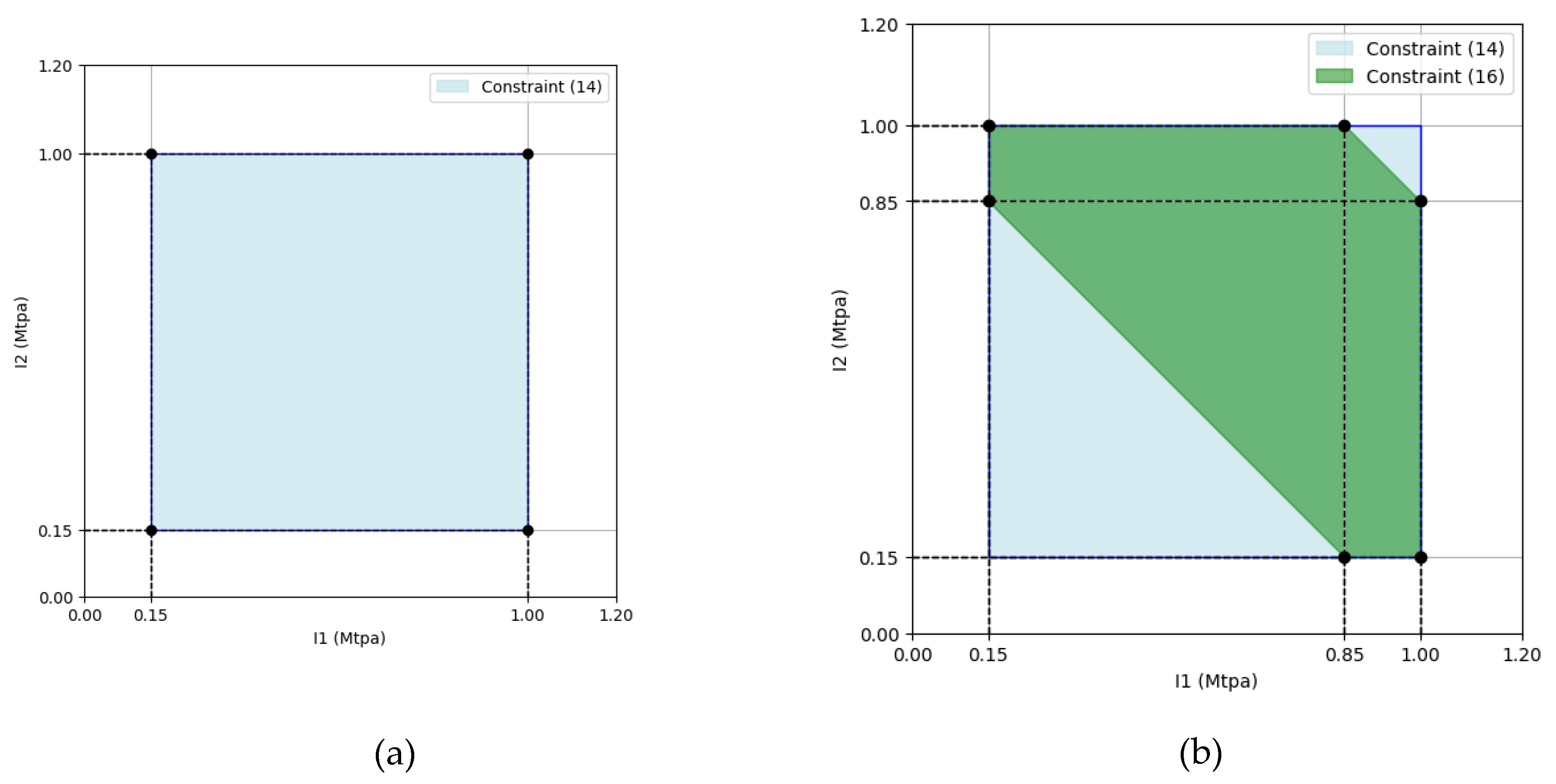
Figure 2.
Case studies aquifer depth.
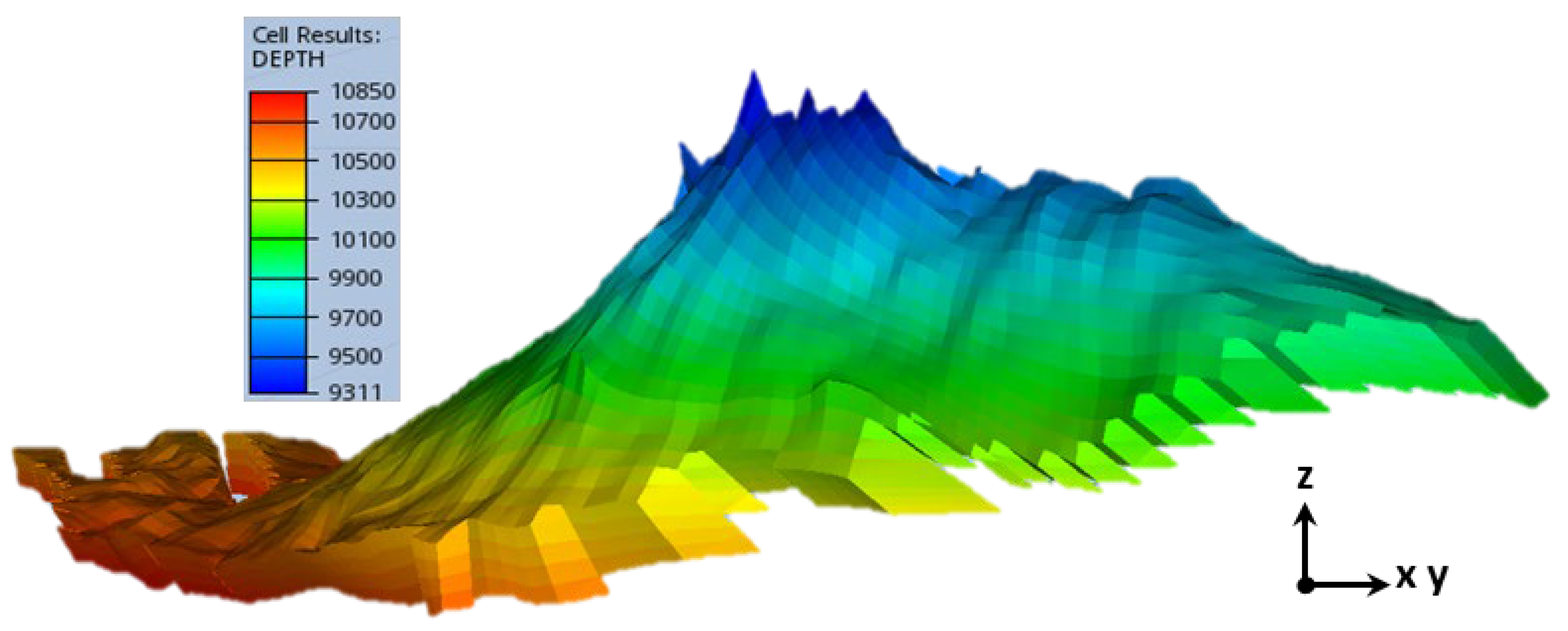
Figure 3.
Aquifer grid block permeability in X direction.
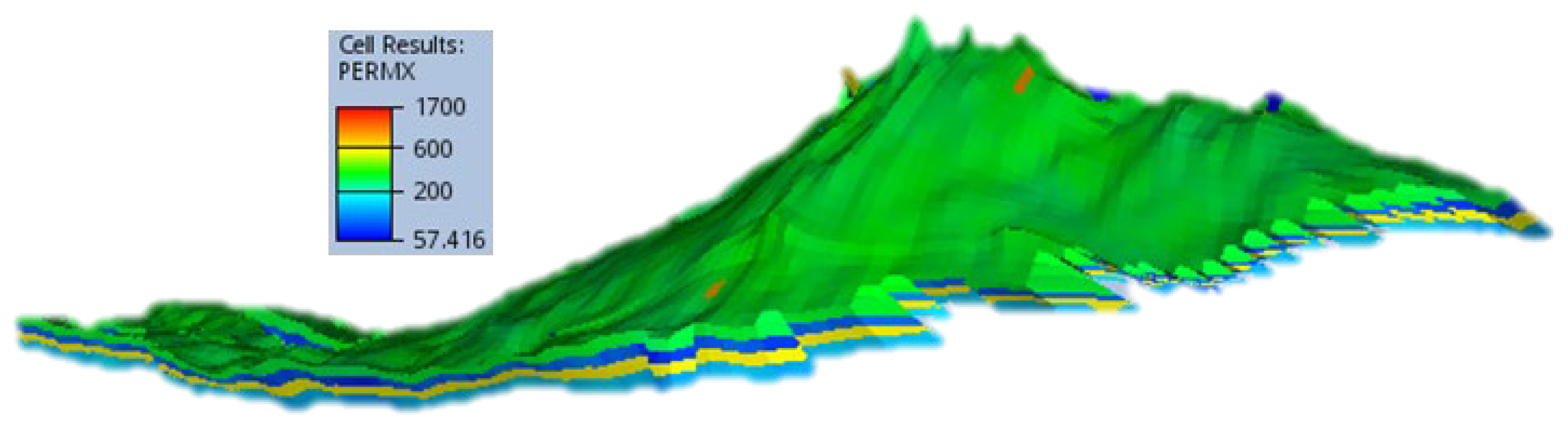
Figure 4.
CO2- brine relative permeabilities plot.
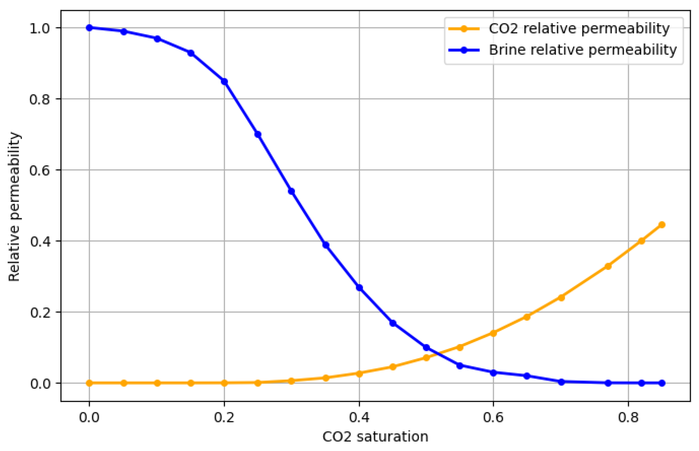
Figure 5.
Injection and production optimal well placement in the modeled aquifer (Fotias, Ismail, & Gaganis, 2024).
Figure 5.
Injection and production optimal well placement in the modeled aquifer (Fotias, Ismail, & Gaganis, 2024).
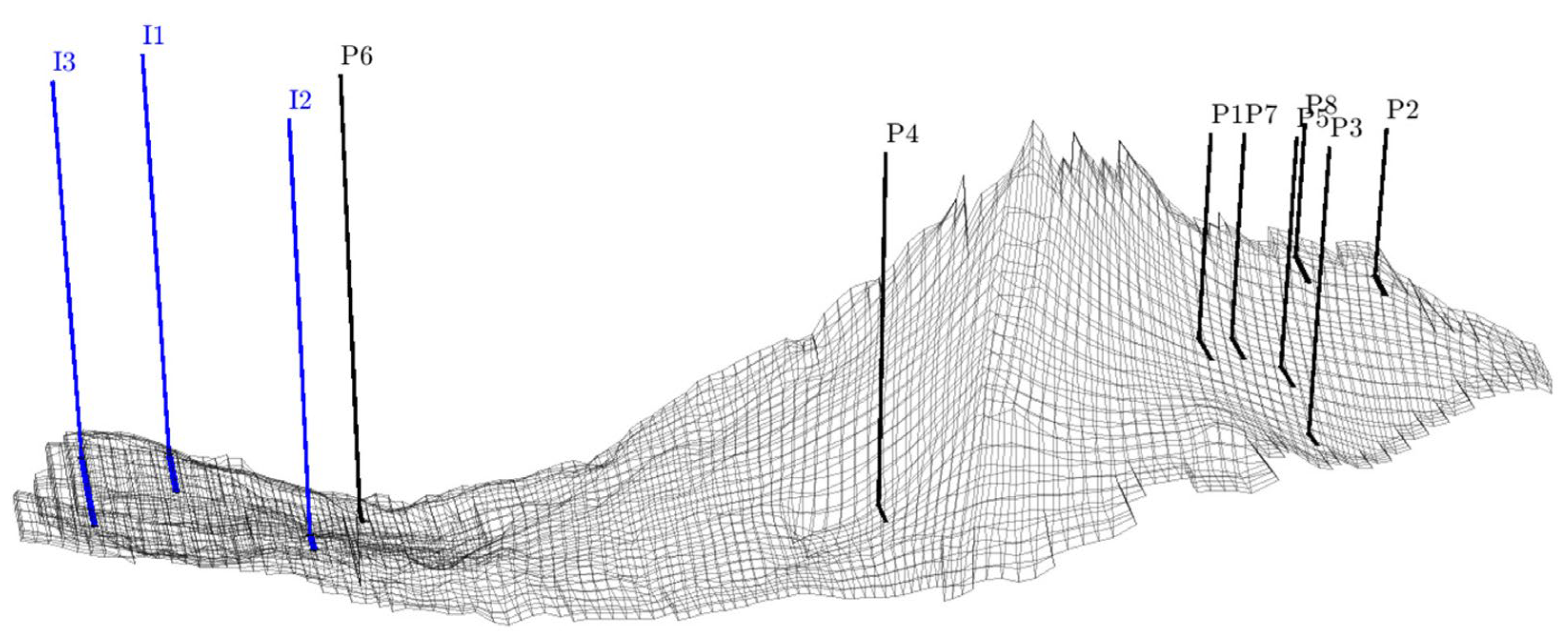
Figure 6.
The feasible design areas together with the placement of the design points for the first (a) and the second (b) case respectively.
Figure 6.
The feasible design areas together with the placement of the design points for the first (a) and the second (b) case respectively.
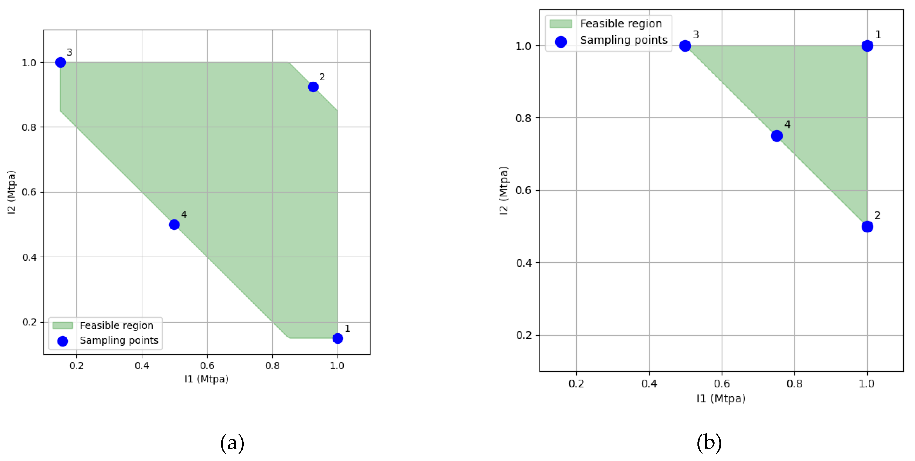
Figure 7.
Response surface of the system within the feasible region (light green) and outside the feasible space, modeled using a second-order surrogate with interaction effects.
Figure 7.
Response surface of the system within the feasible region (light green) and outside the feasible space, modeled using a second-order surrogate with interaction effects.
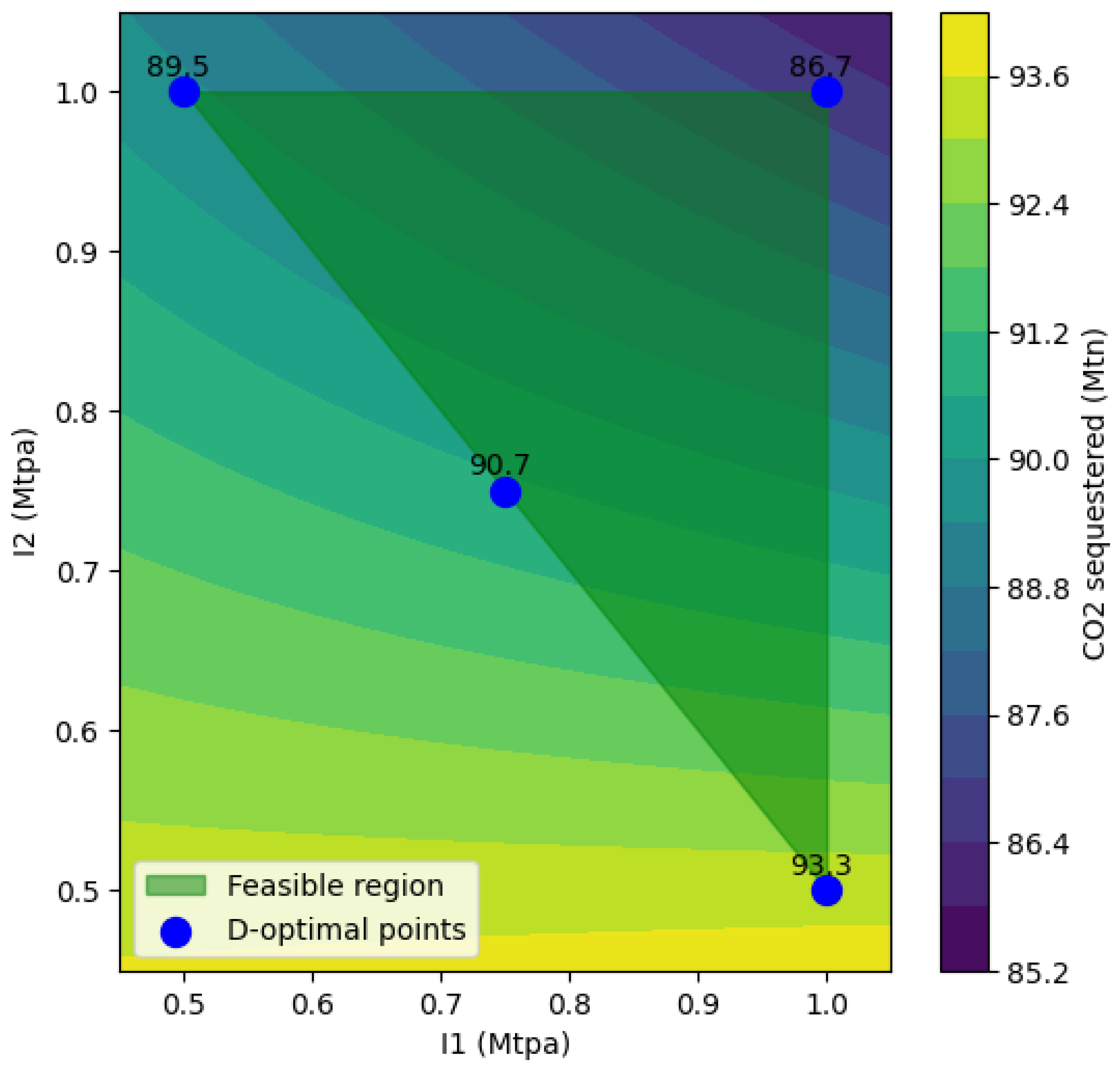
Figure 8.
Surrogate model of CO₂ sequestration constructed from the D-optimal design points, overlaid with the targeted 100 Mtn CO₂ plane. The figure illustrates the predicted sequestration surface within the feasible design space, highlighting the alignment of the surrogate model with the D-optimal points and the location of the target plane.
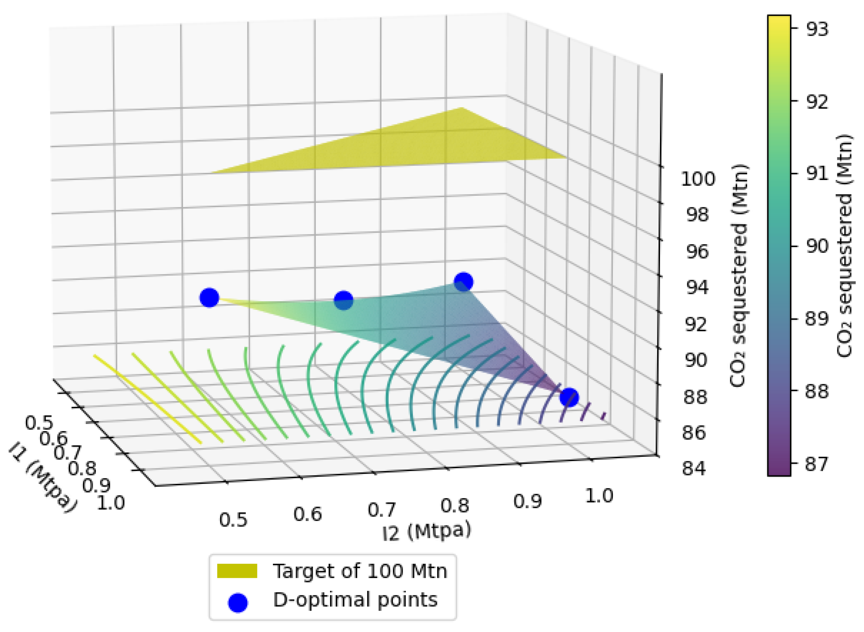
Figure 9.
Distribution of CO₂ saturation at four distinct time steps: t = 10 years, t = 20 years, t = 30 years, and t = 40 years. The figure illustrates the spatial evolution of the CO₂ plume over time.
Figure 9.
Distribution of CO₂ saturation at four distinct time steps: t = 10 years, t = 20 years, t = 30 years, and t = 40 years. The figure illustrates the spatial evolution of the CO₂ plume over time.
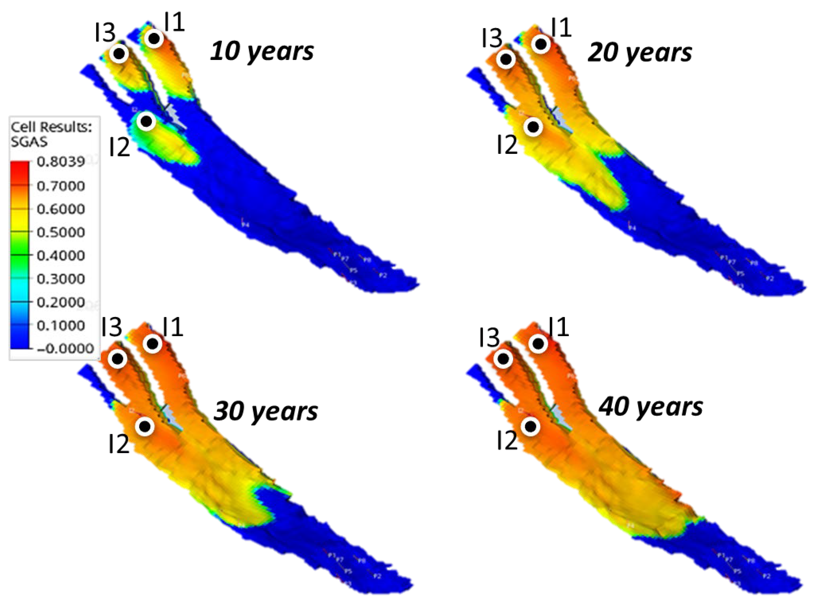
Figure 10.
Distribution of pressure build up at the end of the project: t = 40 years.
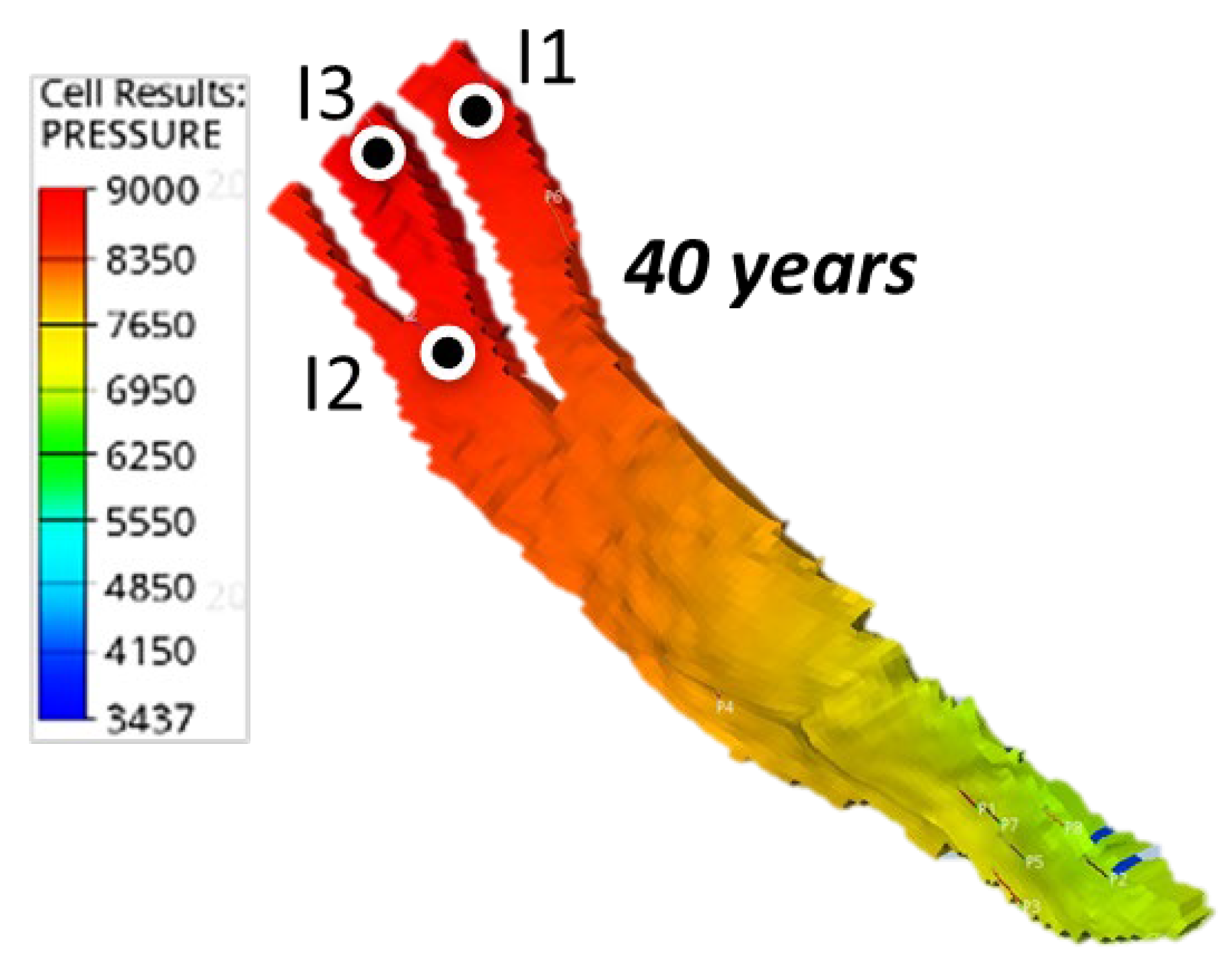
Figure 12.
Field performance profiles: Average reservoir pressure.
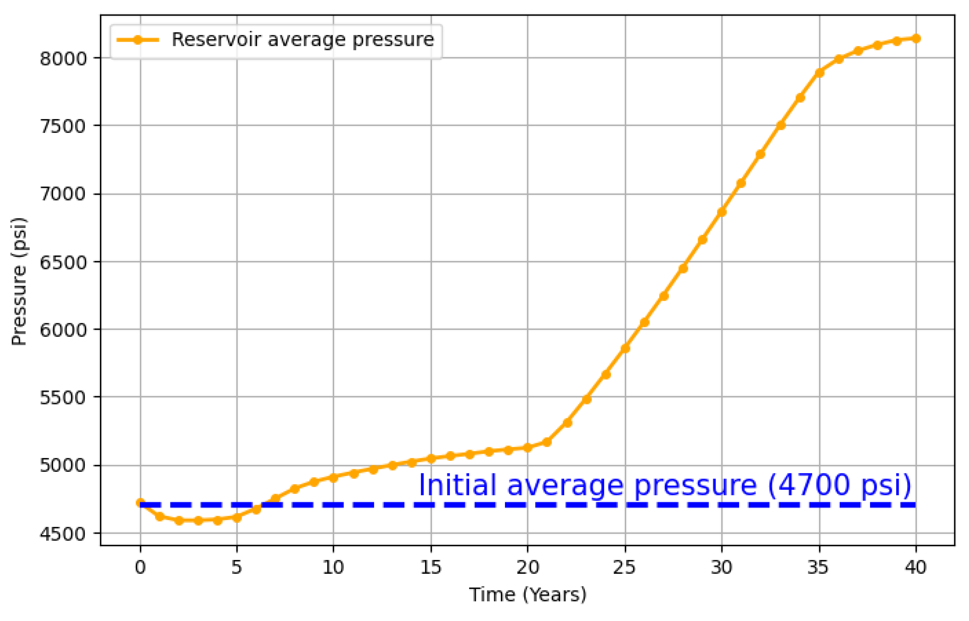
Figure 12.
Field performance profiles: CO₂ injection rate (blue) and CO₂ field recycled (red).
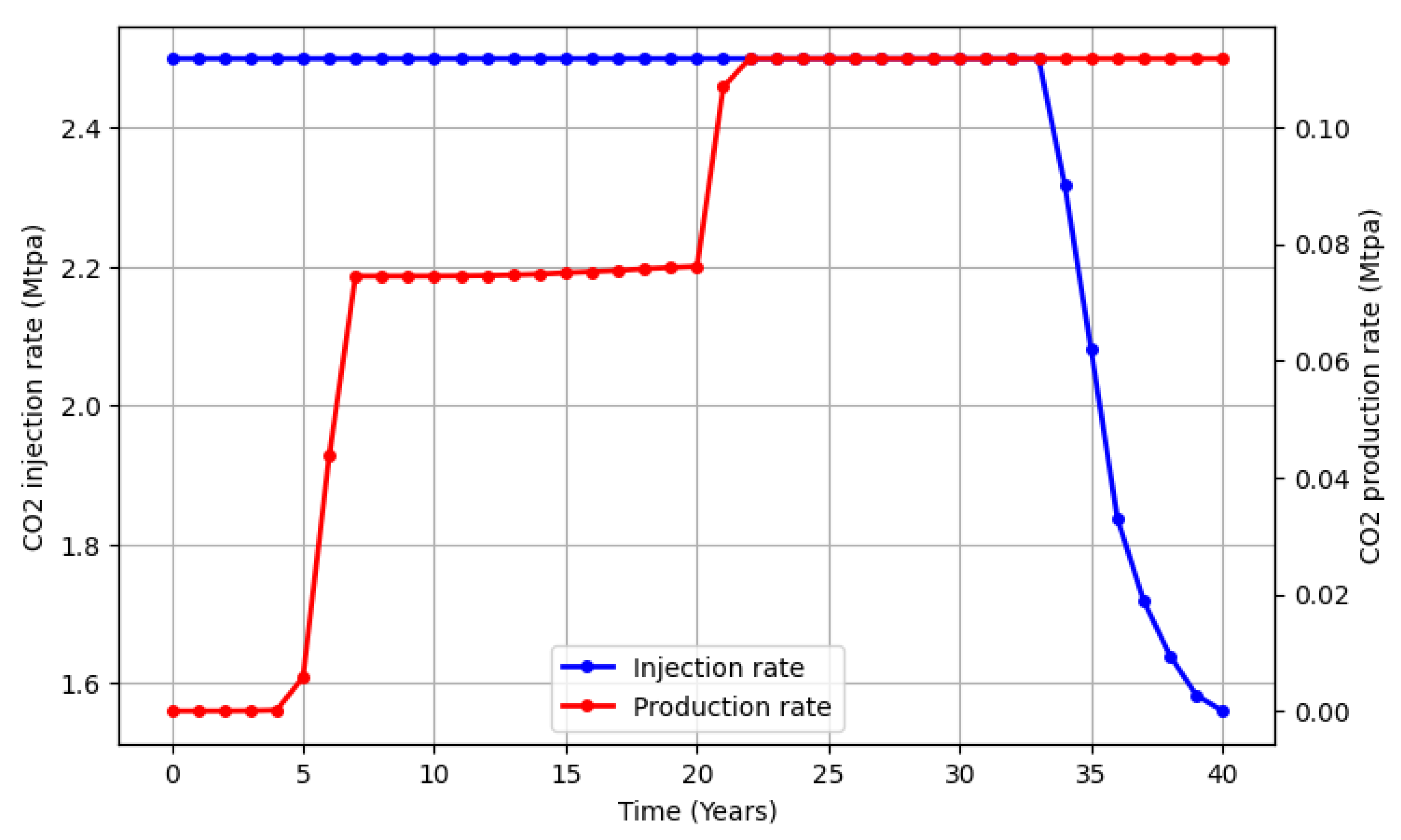
Figure 13.
Performance profiles by well: Bottom-hole pressures of wells I₁, I₂, and I₃ over the 40-year injection period.
Figure 13.
Performance profiles by well: Bottom-hole pressures of wells I₁, I₂, and I₃ over the 40-year injection period.
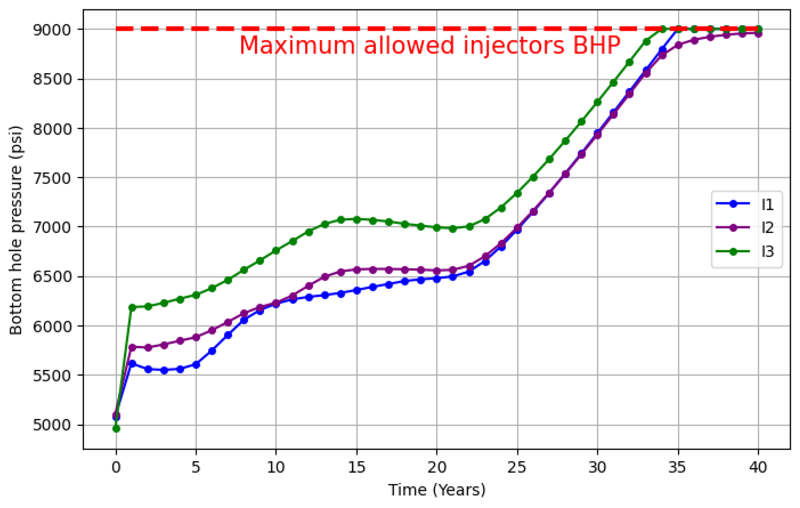
Figure 14.
Performance profiles by well: Injection rates of wells I₁, I₂, and I₃ over the 40-year injection period.
Figure 14.
Performance profiles by well: Injection rates of wells I₁, I₂, and I₃ over the 40-year injection period.
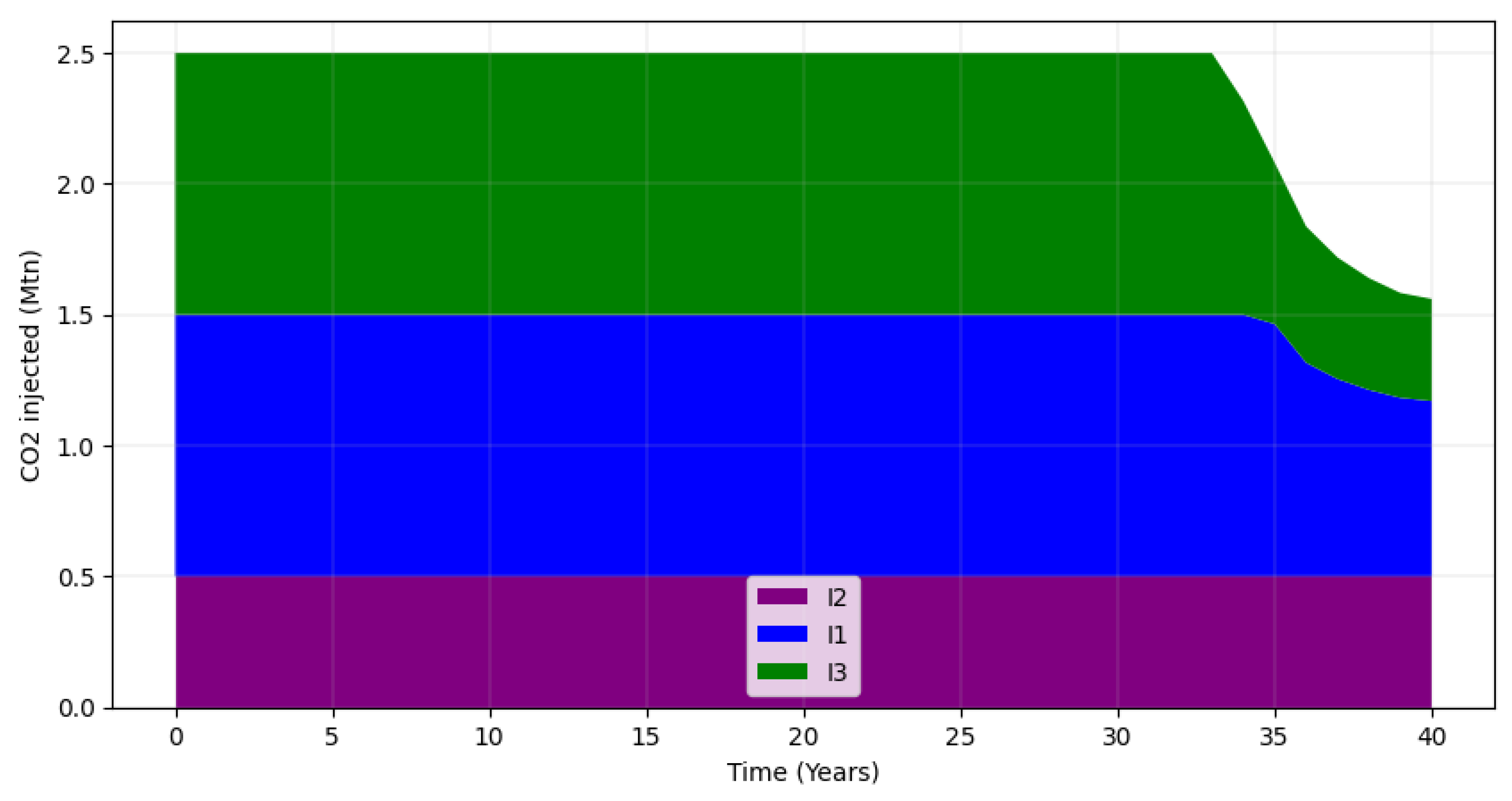
Figure 15.
The plot shows the placement of the nine D-optimal design points (blue) and the relative position of the final near-optimal solution (red) obtained from the optimization methodology.
Figure 15.
The plot shows the placement of the nine D-optimal design points (blue) and the relative position of the final near-optimal solution (red) obtained from the optimization methodology.
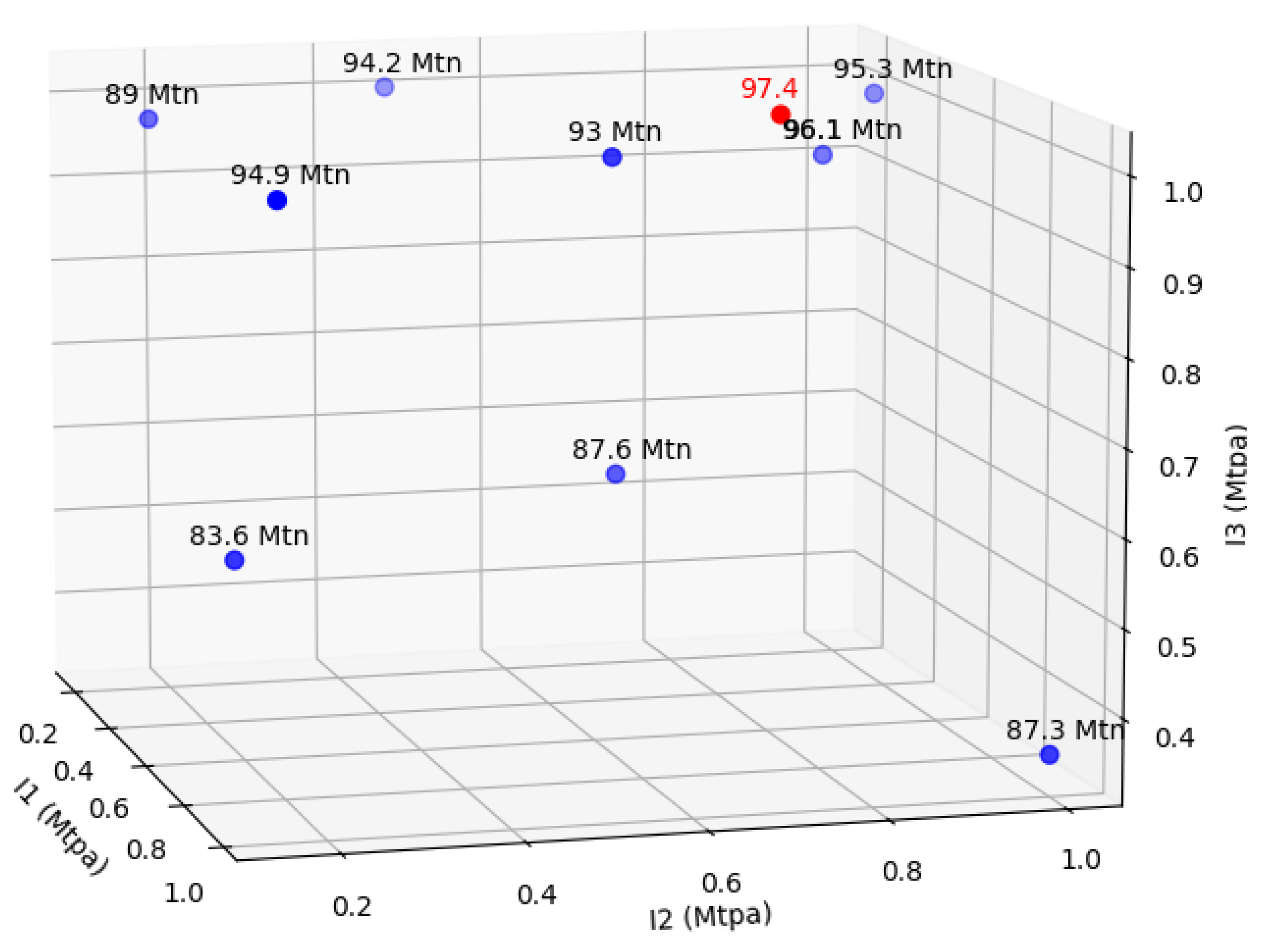
Figure 16.
Plot illustrating the optimization path of the γ parameter. Step 0 represents the RBF surrogate constructed from the nine D-optimal points. Points 1 through 6 indicate each γ optimization step, with the procedure concluding at the 15th point (the 6th optimization step).
Figure 16.
Plot illustrating the optimization path of the γ parameter. Step 0 represents the RBF surrogate constructed from the nine D-optimal points. Points 1 through 6 indicate each γ optimization step, with the procedure concluding at the 15th point (the 6th optimization step).
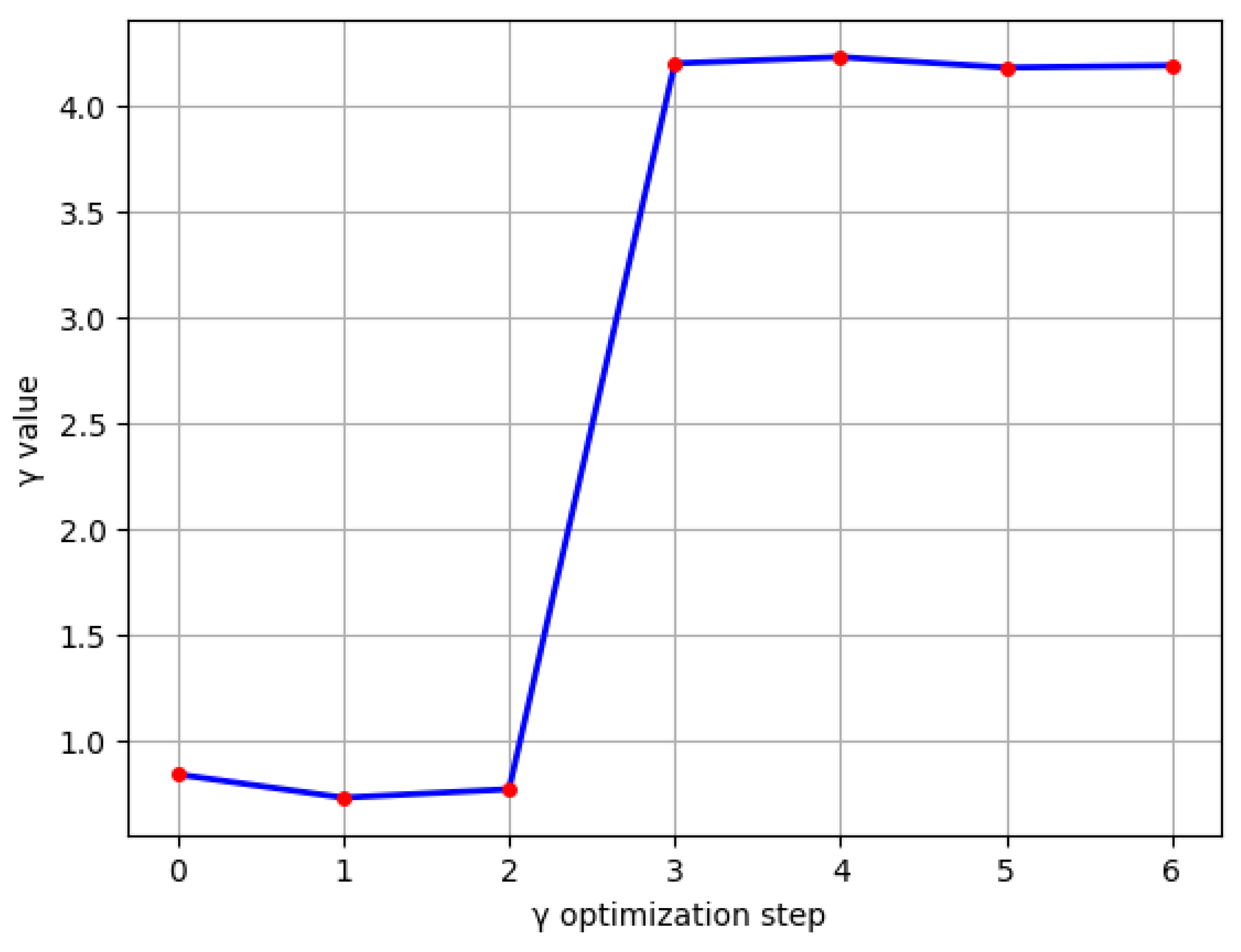
Figure 17.
Plot demonstrating the influence of the γ parameter (eight different cases) on the absolute total error of the five testing points (expressed as relative error, %).
Figure 17.
Plot demonstrating the influence of the γ parameter (eight different cases) on the absolute total error of the five testing points (expressed as relative error, %).
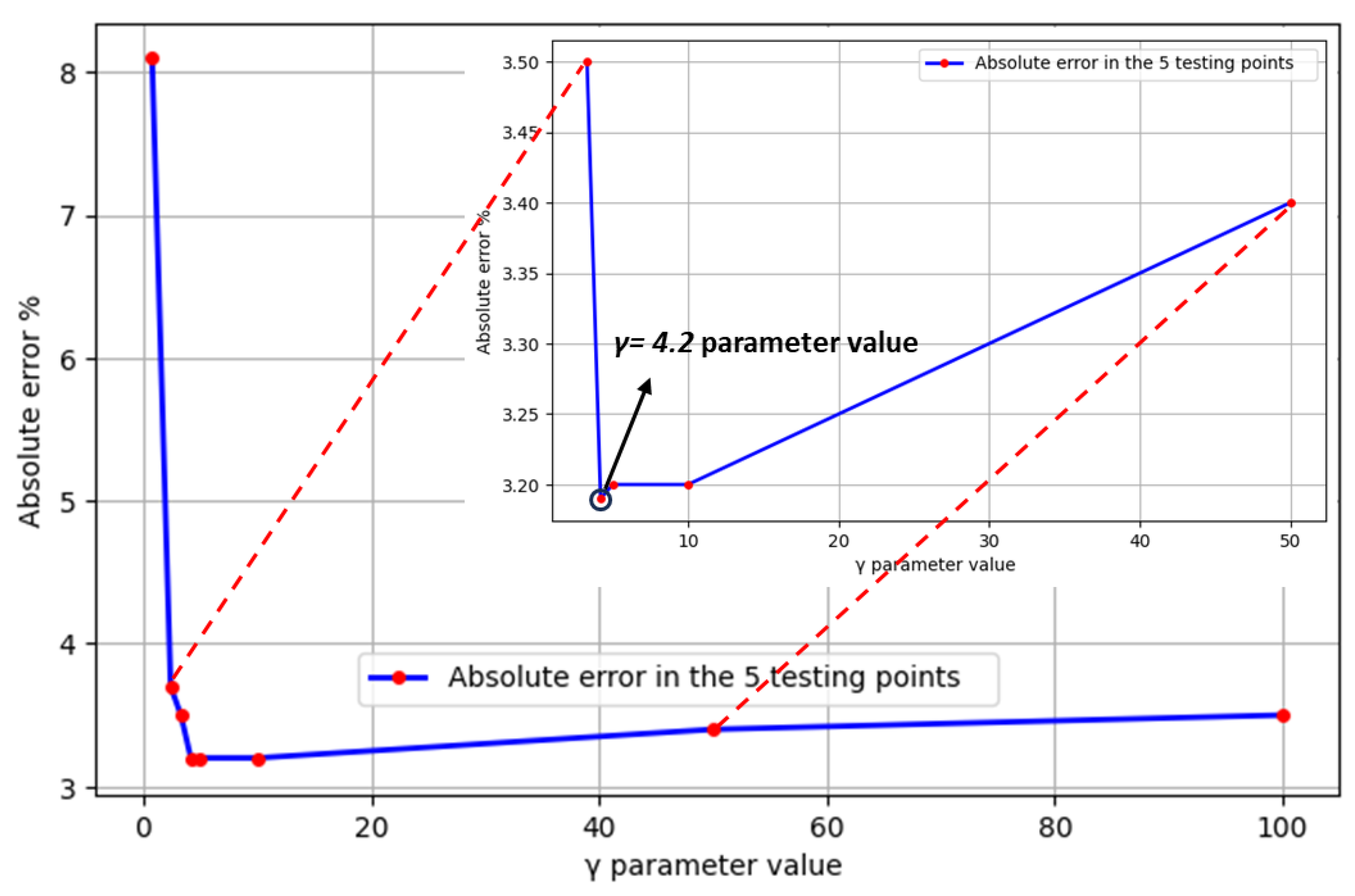
Figure 18.
3D distribution of CO₂ saturation at t = 10 years, t = 20 years, t = 30 years, and t = 40 years.
Figure 18.
3D distribution of CO₂ saturation at t = 10 years, t = 20 years, t = 30 years, and t = 40 years.
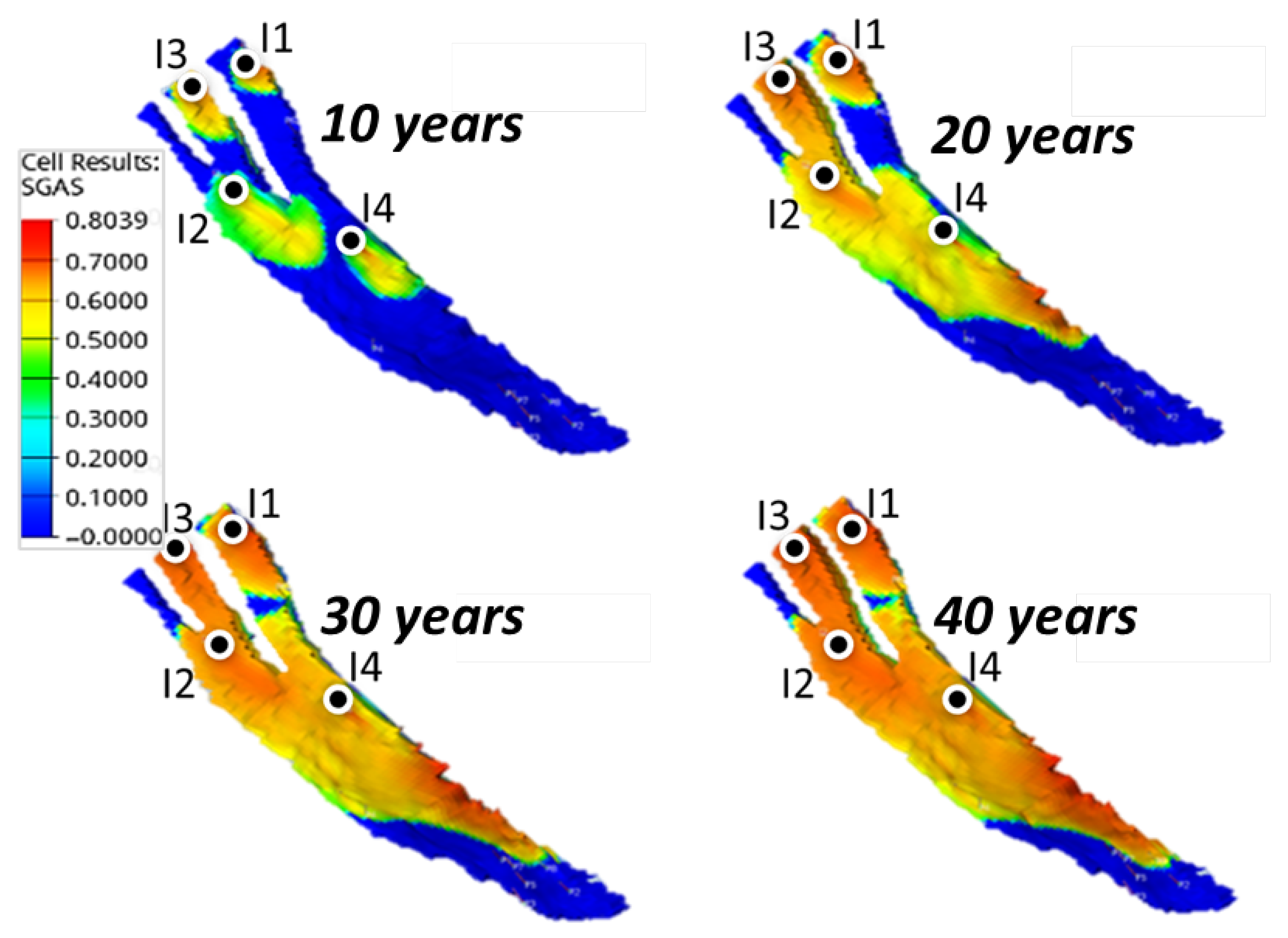
Figure 19.
Distribution of pressure build up at the end of the project at t = 40 years.
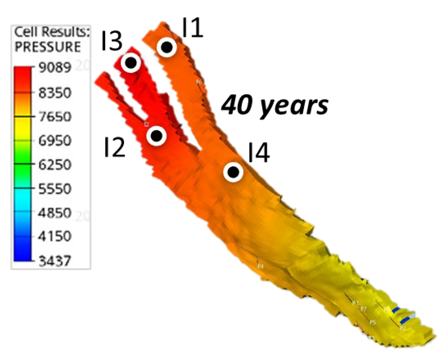
Figure 20.
Field performance profiles: Average reservoir pressure.
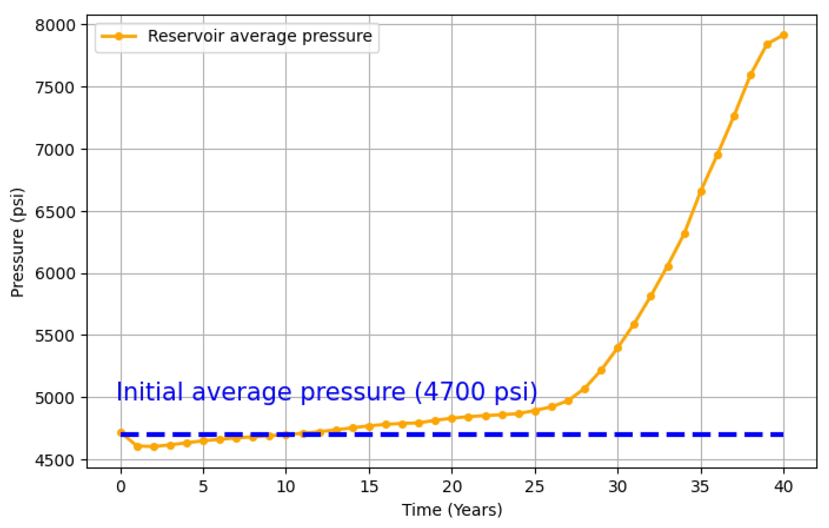
Figure 21.
Field performance profiles: CO₂ injection rate (blue) and CO₂ field recycled (red).
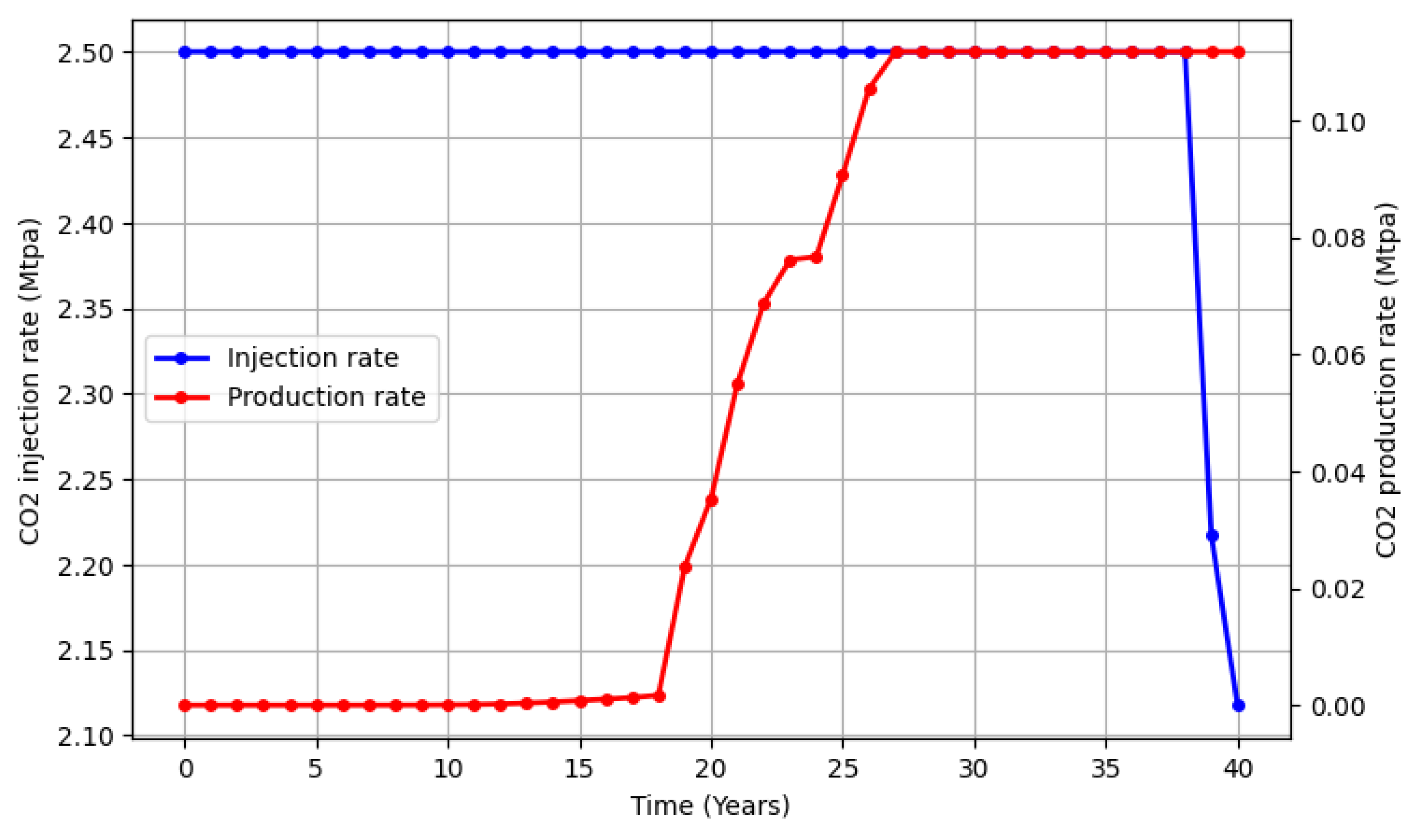
Figure 22.
Performance profiles by well: Bottom-hole pressures of wells I₁, I₂, I₃ and I4 over the 40-year injection period.
Figure 22.
Performance profiles by well: Bottom-hole pressures of wells I₁, I₂, I₃ and I4 over the 40-year injection period.

Figure 23.
Performance profiles by well: Injection rates of wells I₁, I₂, I₃ and I4 over the 40-year injection period.
Figure 23.
Performance profiles by well: Injection rates of wells I₁, I₂, I₃ and I4 over the 40-year injection period.
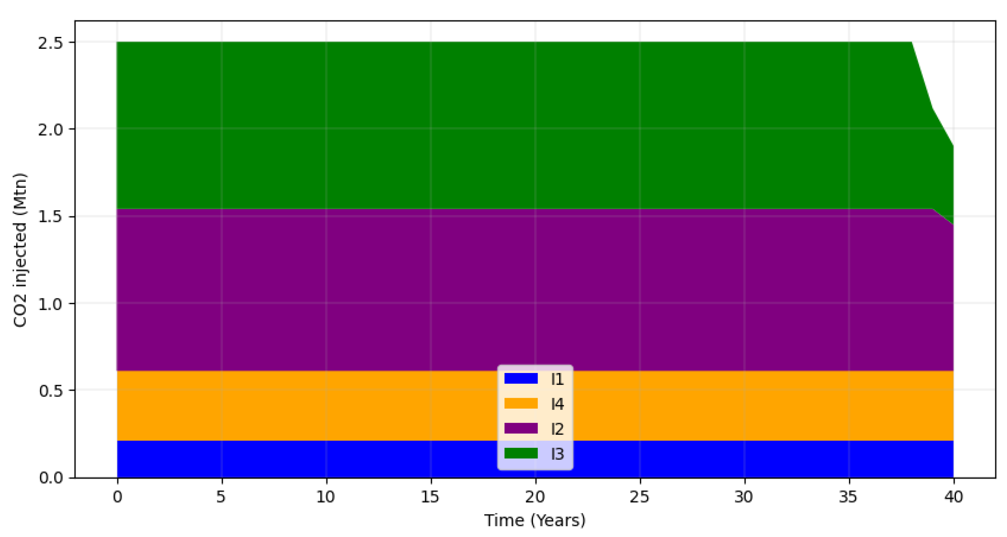
Table 1.
Operational specifications of field wells and well groups.
| Group | Maximum brine production (Mstb/day) | Maximum CO2 production (MMscf/day) |
BHP limits (psi) |
| Field | 80 | 6.0 | - |
| Producers | 60 | 4.0 | 3,000 |
| Injectors | - | - | 9,000 |
Table 2.
D-optimal design observations of I1 I2 (Mtpa), and simulated (Mtn).
| I1 (Mtpa) | I2 (Mtpa) | (Mtn) |
| 1.00 | 1.00 | 80 |
| 1.00 | 0.50 | 80 |
| 0.50 | 1.00 | 80 |
| 0.75 | 0.75 | 80 |
Table 3.
D-optimal design observations of I1 I2 (Mtpa), and simulated (Mtn).
| I1 (Mtpa) | I2 (Mtpa) | (Mtn) |
| 0.75 | 0.75 | 90.7 |
| 1.00 | 0.50 | 93.3 |
| 0.50 | 1.00 | 89.5 |
| 1.00 | 1.00 | 86.7 |
Table 4.
D-optimal design observations with corresponding values of (Mtpa), and simulated CO₂ sequestration (Mtn).
Table 4.
D-optimal design observations with corresponding values of (Mtpa), and simulated CO₂ sequestration (Mtn).
| Point | ξ= (I1, I2, I3, I4) (Mtpa) | (Mtn) |
| 1 | (0.35, 1.00, 1.00, 0.15) | 95.3 |
| 2 | (0.35, 0.15, 1.00, 1.00) | 89.0 |
| 3 | (0.78, 0.15, 0.57, 1.00) | 83.6 |
| 4 | (0.15, 0.47, 1.00, 0.88) | 94.2 |
| 5 | (1.00, 0.15, 1.00, 0.35) | 94.9 |
| 6 | (0.15, 1.00, 0.90, 0.45) | 96.1 |
| 7 | (0.65, 0.61, 0.62, 0.62) | 87.6 |
| 8 | (1.00, 1.00, 0.35, 0.15) | 87.3 |
| 9 | (0.78, 0.57, 1.00, 0.15) | 93.0 |
Table 5.
Step-by-step optimization with corresponding values of (Mtpa), parameter optimization and simulated CO₂ sequestration (Mtn).
Table 5.
Step-by-step optimization with corresponding values of (Mtpa), parameter optimization and simulated CO₂ sequestration (Mtn).
| Point | (I1, I2, I3, I4) (Mtpa) | γ | (Mtn) |
| 10 | (0.15, 0.92, 1.0, 0.43) | 0.73 | 96.8 |
| 11 | (0.15, 0.95, 1.0, 0.40) | 0.77 | 96.7 |
| 12 | (0.15, 0.85, 1.0, 0.50) | 4.20 | 96 |
| 13 | (0.21, 0.93, 0.96, 0.40) | 4.23 | 97.4 |
| 14 | (0.21, 0.93, 0.96, 0.40) | 4.18 | 97.4 |
| 15 | (0.21, 0.93, 0.96, 0.40) | 4.19 | 97.4 |
Table 6.
Cases comparison table.
| Case | Number of injectors | Targeted CO2 sequestration (Mtn) | Achieved CO2 sequestration (Mtn) | D-optimal design points | Simulations required |
| Case 1 | 3 | 80 | 80 | 4 | 4 |
| Case 2 | 3 | 100 | 93.3 | 4 | 5 |
| Case 3 | 4 | 100 | 97.4 | 9 | 15 |
Disclaimer/Publisher’s Note: The statements, opinions and data contained in all publications are solely those of the individual author(s) and contributor(s) and not of MDPI and/or the editor(s). MDPI and/or the editor(s) disclaim responsibility for any injury to people or property resulting from any ideas, methods, instructions or products referred to in the content. |
© 2025 by the authors. Licensee MDPI, Basel, Switzerland. This article is an open access article distributed under the terms and conditions of the Creative Commons Attribution (CC BY) license (http://creativecommons.org/licenses/by/4.0/).
Copyright: This open access article is published under a Creative Commons CC BY 4.0 license, which permit the free download, distribution, and reuse, provided that the author and preprint are cited in any reuse.


