
Submitted:
22 December 2025
Posted:
23 December 2025
You are already at the latest version
Abstract
An $n$-color composition is a colored composition in which a part of size $m$ may come in $m$ colors. This paper gives a new set of $n$-color-type compositions that admits exhaustive conjugation of its members. Previous attempts at conjugation of $n$-color compositions have yielded partial results at best. Instead of importing the coloring scheme previously used for partitions, we apply colors directly to the parts of compositions while treating any maximal string of 1's as a single part under color assignment. This leads to the definition of $n$-color compositions of the second kind. As with ordinary compositions a conjugate may be found by the equivalent techniques of symbolic algebra, zig-zag graph and line graph. We conclude with a derivation of the relevant enumeration formulas.
Keywords:
composition
; conjugate
; zig-zag graph
; line graph
; symbolic algebra
MSC: 11P81; 05A17; 05A15
1. Introduction
A composition of a positive integer n is an ordered partition of n or a sequence of positive integers that sum to n. The summands are also called parts and n is the weight of the composition. For example, has four compositions: and . It is well known that there are compositions of n (see for example [5,7]).
Colored compositions are generalized compositions in which a part size may come in a prescribed number of types or colors, usually denoted by subscripts, . In particular, an n-color composition is a colored composition in which a part of size m may come in m colors: ,1]. For example, there are eight n-color compositions of 3, namely
The n-color notion originated from a paper of Agarwal and Andrews [2] that investigated combinatorial identities for “partitions with n copies of n”, that is, n-color partitions. Subsequently Agarwal [1] defined n-color compositions and explored their enumeration and combinatorial properties. For instance, he proved that the number of n-color compositions of a positive integer is given by , where the Fibonacci numbers are defined by .
The conjugate of a composition is given by the composition corresponding to the columns of its zig-zag graph, read from left to right. For example, the zig-zag graph of is shown in Figure 1.
Thus the conjugate , from Figure 1, is . Two further methods of obtaining are mentioned below.
It appears that the n-color compositions cannot all be conjugated like ordinary compositions! Brian Hopkins [8] made a limited attempt by means of zig-zag graphs and concluded that only certain compositions with odd weights and parts not exceeding 3 may be conjugated. A year later, Collins et al. [6] discussed the topic briefly using tilings of 1-by-n boards with ternary sequences, and gave few instances. However, their technique was rather elusive, and no counting formula was provided. Alanazi et al. [4] undertook a systematic investigation of the topic using n-multicolor compositions with tilings of 1-by-n boards and ternary sequences. They modeled their technique after an extension of MacMahon’s line graph conjugation method, and discovered a remarkably large set of conjugable n-color compositions.
Theorem 1
(Alanazi et al. [4]). The number of conjugable n-color compositions of an integer is given by .
However, even in the latter model, a substantial number of objects still escaped conjugation. Note that for all .
Lastly, we refer to a significant 1997 paper of Agarwal and Balasubrananian [3] where the conjugate of an n-color partition is defined as the n-color partition obtained by replacing each colored part by . The authors used this definition to establish an identity between “n-color partitions where the weighted difference of each pair of parts is ” and “n-color partitions such that in each pair of parts () b is the arithmetic mean of the subscripts i and j”, among other results.
One may apply this definition to n-color compositions and obtain the conjugate of every object! We will refer to this conjugation as color-complement or simply c-complement. For example, if , then the c-complement conjugate is given by .
Proposition 1.
The number of c-complement self-conjugate n-color compositions of ν is given by .
Since maps to and , self-conjugate parts are odd parts () with each part subscripted by its unique numerical index among increasing odd positive integers. The result then follows from the fact that compositions of into odd parts are enumerated by (see [7,11]). For example, is c-complement self-conjugate.
Even though c-complement conjugation admits conjugation of every n-color composition C, the parts of C and remain rigidly the same, and it is not clear how can be found graphically. Nonetheless, the method holds independent interest and may be gainfully applied to any set of subscripted integer sequences.
This paper introduces a modified set of n-color compositions in which every object has a conjugate in the classical tradition of Percy Alexander MacMahon (1854–1929) who pioneered the topic for ordinary compositions. Whereas standard n-color compositions originated by extending to compositions the coloring scheme used for partitions (see [1,2]), our objects arise from coloring compositions directly. Such colored compositions share the essential property of n-color compositions by requiring that a subscript associated with a part cannot exceed the part.
In Section 2 we profile the new set of conjugable colored compositions with some immediate examples. Then in Section 3 we give further details of three conjugation techniques gleaned from the conjugation of ordinary compositions. Section 4 is devoted to the statement and proof of relvant enumeration formulas. Finally, Section 5 contains additional enumeration results for objects with parts sizes bounded from below.
2. The n-Color Compositions of the Second Kind
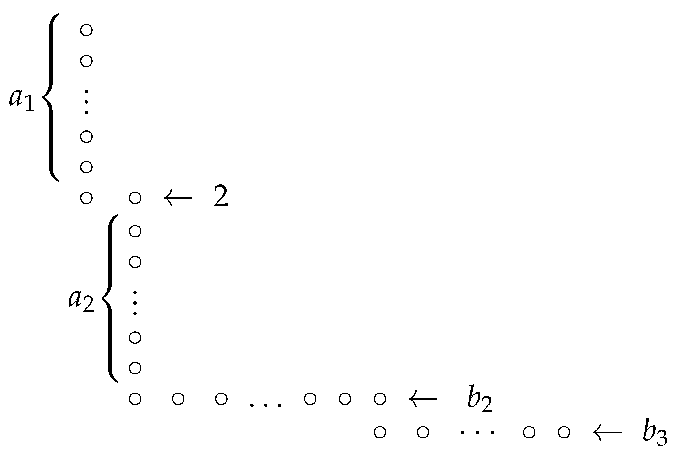
It will be convenient to write compositions, symbolically, by representing a maximal string of 1’s of length x by , where two adjacent big parts (i.e., parts ) are assumed to be separated by . A general composition then has one of the following two forms:
where it is understood in each case that C either ends in or for some with and .
The first or last part of a composition C will also be referred to as a boundary part. Any other part of C is an interior part.
In defining our new set of colored compositions, we will be guided by the conjugation model of P. A. MacMahon for ordinary compositions, that is, every composition C has a unique conjugate that satisfies the following conditions:
(i) is obtainable from C via symbolic algebra;
(ii) is obtainable from the line graph of ; and
(iii) is obtainable from the zig-zag graph of C.
For example, besides the zig-zag graph technique shown earlier, one may use symbolic algebra and the line graph to obtain as fo llows.
Firstly, the symbolic algebra conjugation of is given by
Thus an interior part conjugates to . We will also refer to as the number of interior units of m. Note that 2 conjugates to and so has 0 interior units.
For example, has the conjugate
For the line graph we use circular nodes separated by bars (instead of line segments separated by dots). Thus we get
By deleting the bars and placing bars inside the gaps that previously had none, we obtain
from which we read off the conjugate as .
We now propose an n-color-type scheme that satisfies the three conjugation conditions. Our most significant departure from standard n-color compositions is a negation of the assignment of the color 1 to each part 1 in every maximal string . It is known that an ordinary composition generates as many n-color compositions as the product of its parts (see, for example, [13]). For example, generates the following 6 objects.
Indeed any composition of the form generates exactly 6 n-color compositions.
The coloring scheme proposed here accounts for the fact that the number of colors of a part-size m is dominated by m. But we treat a string of m ones, , , as the single part m with respect to color assignment. This is informed by the conjugation of standard compositions in which strings of 1’s translate into big parts.
This makes sense because a boundary string conjugates into the boundary part (which is entitled to colors) while an interior string conjugates into the interior part (which is entitled to colors). We see that an assignment of just the single color 1 to , independent of the size of x, is not symmetrical.
This color assignment is also supported by the natural fact that the parts of a composition occur as an ordered sequence. Thus in the proposed model, a colored part occurs in a composition if and only if a corresponding string , occurs in the ordinary support composition if and only if a string of x colored parts , actually occur in . Thus, for instance, if is colored 2 in a composition, these will appear as or in the symbolic form .
Another seemingly unusual assignment is that when 2 occurs as an interior part it has no color (or empty color) denoted by . This is justified by the naturally derived conjugation principle:
“a big part bears a positive color if and only if it can be obtained via a symbolic transformation of a string of 1’s with a positive color by conjugation".
It is clear that 2 does not fulfill this condition because it is obtained by transforming a zero string of ones under conjugation (see the paragraph immediately following (3)).
Suppose C is a composition of . Let and denote the respective sets of possible colors of a boundary and interior big part , and let and denote the sets of possible colors of a boundary and interior string of ones .
Definition 1.
Let C be an ordinary composition of ν. A conjugable n-Color Composition is any colored composition of ν obtained by applying the following color assignments to the parts of C.
If C is a trivial composition, that is, , then each symbolic part admits ν colors:
- ;
Otherwise,
- (i)
- ;
- (ii)
- ;
- (iii)
- ;
- (iv)
- .
As with ordinary compositions, the LG nodes of a boundary part (or boundary string of 1’s) are read from left to right on the left boundary, and from right to left on the right boundary.
Remark 1.
Note that when standard n-color compositions are defined with respect to sets of colors assigned to the parts of an ordinary composition, we have
Using the line graph, colors will be assigned to interior units of interior big parts. Thus an interior part represented by b nodes in a line graph is assigned a color only at one of the interior nodes, that is, at one of the 2nd to the th nodes:
Secondly, a left boundary part is assigned a color only at one of the first nodes (similarly for a right boundary part):
On the other hand, it is clear that 2 with the representation has no interior unit. So an interior part 2 bears the color 0. However, a boundary part 2, with a representation of the form or , clearly has one colorable node, on the left or on the right, respectively. Consequently, in a nontrivial conjugable n-color composition 2 always takes the boundary form and the interior form .
Finally, we remark that a string of 1’s, being already units, may be assigned a color at any of its nodes in a line graph.
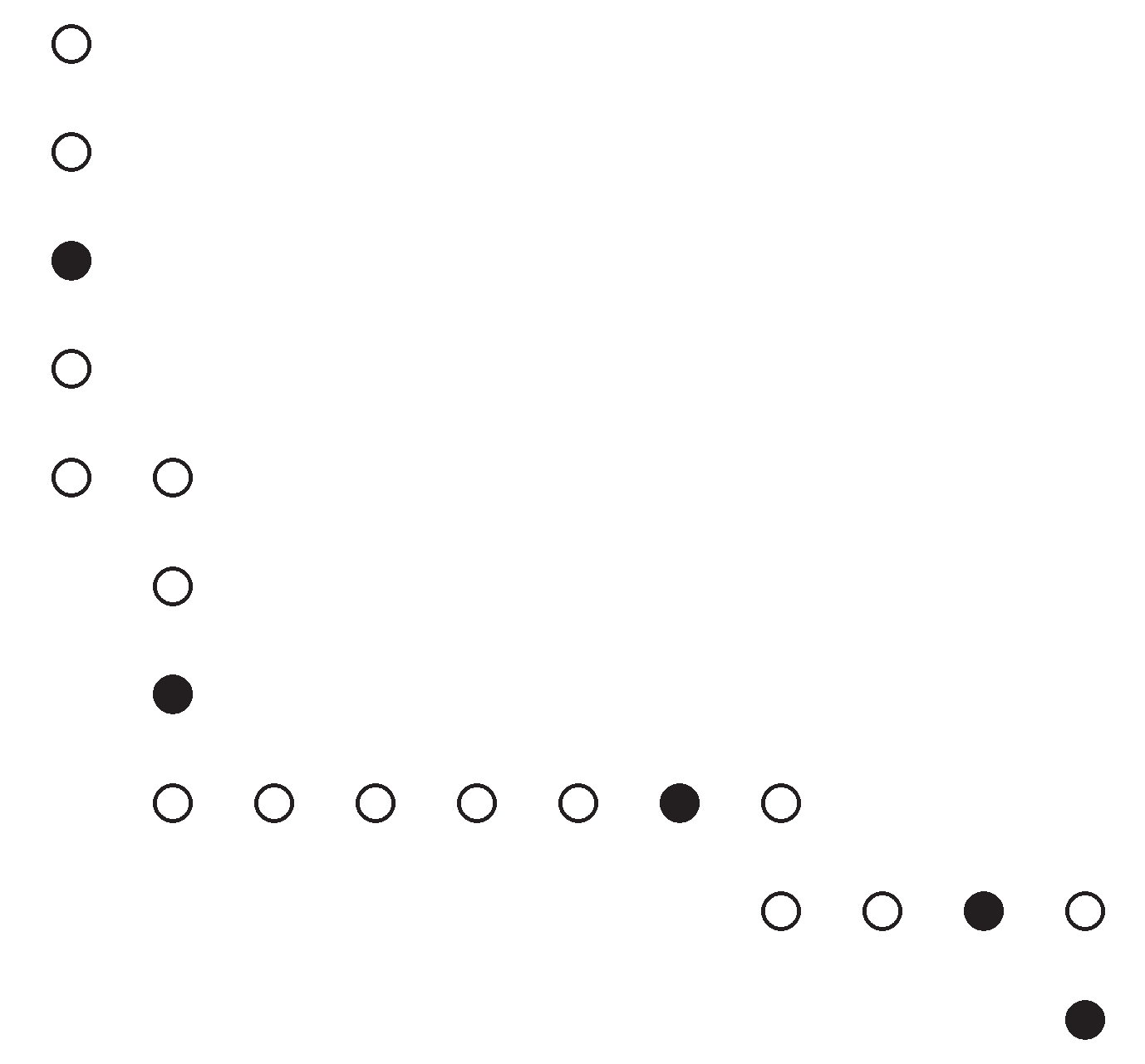
These facts may also be depicted using a zig-zag graph. For example, consider the composition . From the zig-zag graph in Figure 2, it is intuitively clear why any of the (or ) nodes is colorable, why neither of the 2 interior nodes can be colored, why only the second to the th nodes are colorable, and why only the last nodes are colorable.
With these coloring rules observed, the conjugate of the resulting colored composition may be obtained by reading the diagram by columns, from left to right.
For example, the conjugable n-color composition
has the following zigzag graph representation:
| ∘ | ||||||||
| • | ||||||||
| ∘ | ||||||||
| ∘ | ||||||||
| ∘ | ∘ | |||||||
| ∘ | ||||||||
| ∘ | ||||||||
| • | ||||||||
| ∘ | ∘ | • | ∘ | ∘ | ||||
| ∘ | ∘ | • |
The conjugate is now obtained by reading the zig-zag graph by columns to give . The corresponding line graph of is
The line graph of is obtained by swapping gaps and bars as with ordinary compositions:
Finally, the symbolic algebra technique matches that of ordinary compositions as one may verify by ignoring the colors. Precise details are provided in the next section.
These new colored compositions should be known as n-color compositions of the second kind or simply M-color compositions.
We recap the properties satisfied by an M-color composition based on an ordinary support composition C, as follows. The number of parts of C is denoted by .
- A maximal string of ones of length u comes in u colors, always.
- If C consists of a single part b, then b comes in b colors.
- If , the part comes in one color (namely 1 or 0).
- If and is the first or last part of C, then b comes in colors.
- If is an interior part of C, it comes in colors.
The number of M-color compositions of will be denoted by .
3. The Conjugation Involution
We now give a full explanation of the symbolic algebra technique. The trivial compositions conjugate as follows, for any :
We next convert the ordinary composition C in (1) into a conjugable n-color composition by assigning colors to the parts in accordance with the definition:
Alternatively, (showing the occurrence of 2) let
where the color sizes are subject to the restrictions in (5). Then the conjugate is
Note that the colors in both and satisfy the stipulations in the definition since they immediately agree with (5). For example, in we have for all i, and which gives for , and so forth. Secondly, the conjugation of an interior 2 to and vice-versa are given by convention. Hence the conjugates in (6) and (7) are well-defined.
It is clear that one may similarly assign colors to the parts of the support composition (2) and obtain analogous symbolic conjugates.
We remark that an M-color composition of cannot be self-conjugate, a fact inherited from ordinary (support) compositions (see [12]).
Example 1.
Consider . Then
Alternatively, we may use the line graph and obtain
which, by placing division bars only in gaps which previously had none, leads to
from which the conjugate is again seen to be .
The final approach is to use the the zig-zag graph of as shown below, whence is obtained by reading the graph by columns.
Figure 3.
Zigzag graph of .
Example 2.
If , then which enumerates the following objects (arranged in conjugate pairs):
4. Enumeration of M-Color Compositions
We state the main enumeration result.
Theorem 2.
We have
Proof.
We refer to the list of properties satisfied by the parts of an M-color composition C given at the end of Section 2.
Let and be the generating functions for numbers of M-color compositions with first part 1 and first part respectively.
We first consider the following attributes:
- (i)
- Any maximal string of ones comes in u colours.
- (ii)
- There is exactly one colour for 2 (for now).
- (iii)
- A part comes in colours (for now).
Then is given by an initial block of u ones for which there are u colours, followed by a composition that does not start with 1, that is,
Secondly, is given by either the empty composition of 0, or 2 or an initial part for which there are colours, followed by an arbitrary composition:
Next we account for the further attributes:
- (iv)
- The integer 2 has a second colour if it is the only part.
- (v)
- There is an additional colour for each first or last part .
Thus altogether, (i) to (v) are equivalent to the original conditions (1) to (5) in Section 2.
If we combine the generating functions for (iv) and (v) with Eqn (11), we obtain the full generating function:
This simplifies to
Hence the proof follows. □
The following recurrence is a routine consequence of the generating function (8), and it may be verified that the explicit formula (13) satisfies the recurrence.
Corollary 1.
We have
5. -Color Compositions with Parts Bounded Below
Let denote the number of M-color compositions of that satisfy property P, and let the be the number of those objects wih k parts. We first obtain the generating function for the number of objects without 1’s.
Theorem 3.
We have
Proof.
Note that , that is,
When , each boundary part b has possible colors and each interior part b has colors, while 2 has precisely one color either way. Thus the decomposition is
Therefore,
□
The Case of Objects with Parts
We prove the following assertion.
Theorem 4.
Let be an integer. Then
Proof.
First note that , that is,
When , each boundary part has possible colors and each interior part has colors. Thus the decomposition is
(Note that implies ).
Therefore,
□
6. Discussion
This research introduces a new set of colored compositions endowed with the classical conjugation property of ordinary compositions. Furthermore, there is an enumerative generating function and an explicit computational formula. The results were based directly on the inherent symmetry of compositions. It is worth noting that these M-color compositions also form an interesting class of combinatorial objects in their own right, even without recourse to conjugation. They are expected to become rich objects of research in future. For example, it might be rewarding to examine pattern avoidance questions in the set of M-color compositions. The results of this work will probably be regarded as a significant contribution to the literature of number theory and combinatorics.
Funding
This research received no external funding.
Institutional Review Board Statement
Not applicable.
Data Availability Statement
The colored compositions studied in this paper were computed mostly using the computer algebra system Maple [10]. The relevant codes may be obtained from the author on request.
Acknowledgments
The author thanks Professor Stephan Wagner for generously providing the proof of Theorem 2.
Conflicts of Interest
The author declares no conflict of interest.
References
- A. K. Agarwal, n-color compositions, Indian J. Pure Appl. Math. 2000, 31, 1421–1427.
- Agarwal, A.K.; Andrews, G.E. Rogers-Ramanujan identities for partitions with “N copies of N. J. Combin. Theory Ser. A 1987, 45, No., 40–49. [Google Scholar] [CrossRef]
- Agarwal, A.K.; Balasubramanian, R. n-color partitions with weighted differences equal to minus two. Internat. J. Math. and Math. Sci. 1997, 20(4), 759–768. [Google Scholar] [CrossRef]
- Alanazi, A. M.; Archibald, M.; Munagi, A. O. Multicolor Compositions and Conjugation of N-Color Compositions. Contrib. Discrete Math 2024, 19(3), 68–85. [Google Scholar] [CrossRef]
- Andrews, G. E. The Theory of Partitions, Addison-Wesley, Reading 1976; reprinted; Cambridge University Press: Cambridge, 1984, 1998. [Google Scholar]
- Collins, A.; Dedrickson, C.; Wang, H. Binary words, n-color compositions and bisection of the Fibonacci numbers. Fibonacci Quart. 2013, 51(2), 130–136. [Google Scholar] [CrossRef]
- Heubach, S.; Mansour, T. Combinatorics of Compositions and Words, Discrete Mathematics and its Applications (Boca Raton); CRC Press: Boca Raton, FL, 2010. [Google Scholar]
- Hopkins, B. Spotted tilings and n-color compositions. Integers 2012, 12B, A6. [Google Scholar]
- MacMahon, P.A. : Combinatory Analysis. Cambridge University Press: Cambridge, 1915; Volume 1. [Google Scholar]
- Maple 2020.2. Maplesoft, a division of Waterloo Maple Inc.: Waterloo, Ontario.
- Munagi, A. O. Euler-type Identities for integer compositions via zig-zag graphs. Integers 2012, 12 A60, 10pp. [Google Scholar]
- Munagi, A. O. Primary classes of compositions of numbers. Ann. Math. Inform. 2013, 41, 193–204. [Google Scholar]
- Shapcott, C. C-color compositions and palindromes. Fibonacci Quart. 2012, 50, 297–303. [Google Scholar] [CrossRef]
Figure 1.
Zig-zag graph of .
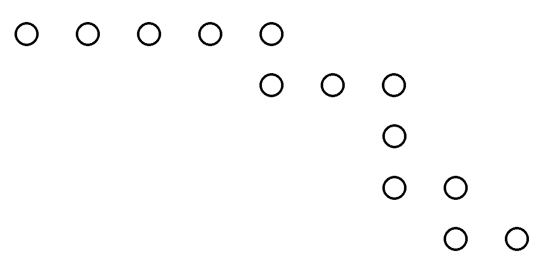
Figure 2.
Zigzag graph of .
Disclaimer/Publisher’s Note: The statements, opinions and data contained in all publications are solely those of the individual author(s) and contributor(s) and not of MDPI and/or the editor(s). MDPI and/or the editor(s) disclaim responsibility for any injury to people or property resulting from any ideas, methods, instructions or products referred to in the content. |
© 2025 by the authors. Licensee MDPI, Basel, Switzerland. This article is an open access article distributed under the terms and conditions of the Creative Commons Attribution (CC BY) license (http://creativecommons.org/licenses/by/4.0/).
Copyright: This open access article is published under a Creative Commons CC BY 4.0 license, which permit the free download, distribution, and reuse, provided that the author and preprint are cited in any reuse.


