Submitted:
31 January 2026
Posted:
02 February 2026
You are already at the latest version
Abstract
In electronic product manufacturing, quality control and production cost man-agement pose challenges for enterprises. First, key factors for production deci-sions are identified: component inspection, assembly, inspection of semi-finished and finished products, and handling defective goods at different stages. Next, dynamic programming and genetic algorithms optimise sampling inspection. A production decision model covers multiple processes and compo-nent combinations. The relationship between the inspection and the final product quality is explored, showing that different decision paths affect the total cost and defect rate. Real-time monitoring and a dynamic Bayesian network guide pro-duction strategy adjustments to boost efficiency and reduce defects. This study proposes adaptable inspection and disassembly strategies that reduce costs and optimise resource use across production scenarios.
Keywords:
electronic products
; production decision-making
; dynamic programming
; dynamic Bayesian network
1. Introduction
With the rapid development of the electronic product manufacturing industry, customer demand for electronic products has gradually increased [1], making quality control and production cost management major challenges faced by enterprises [2,3] The production process of electronic products is relatively complex [4], involving multiple procedures and numerous components [5]. To ensure that customers receive qualified products, quality inspection is a top priority in the production process [6,7]. At various stages, enterprises need to consider the costs and benefits associated with inspection, assembly, disassembly, and after-sales replacement [8,9,10]. Therefore, in a complex production environment, it is necessary to comprehensively consider quality control and cost management to achieve real-time monitoring and dynamic adjustments [11].
Nowadays, many scholars are conducting research on the product manufacturing process. Sarkar and Saren [12] combined Type I and Type II errors, considering the production process in which the system transitions from a controlled state to an uncontrolled state, and adopted a sampling inspection strategy based on inspection errors to ensure product quality. Jing Zhou [13] and others, taking into account that product inspection is influenced by various factors, proposed an improved three-way decision (3WD) approach and introduced a case study in semiconductor manufacturing systems, demonstrating that this method can effectively reduce inspection errors. Tzuan Chiang [1] and others proposed a multi-objective planning method oriented towards customer needs, applying an efficient multi-objective genetic algorithm to achieve maximum customer satisfaction and minimum technical development cost. Qiaochu He [14] and others, based on incorporating the influence of consumer reviews, proposed a new dynamic pricing model to achieve optimal pricing and quality control. You, J [15] and others, for manufacturing systems with multiple machines, multiple product types, and uncertain failures, proposed an integrated control strategy that combines the priority hedging point (PHP) control strategy with capacity planning in the production process to control production costs.
In this study, sampling inspection schemes for the production process of electronic products and decision-making problems under different circumstances were thoroughly investigated. The production process involves component inspection, assembly stages, inspection of semifinished and finished products, and handling of defective products [16,17,18]. Combining methods such as hypothesis testing [18], sequential probability ratio testing [19], dynamic programming, genetic algorithms [20,21], and dynamic Bayesian networks [22], this paper constructs a multi-stage decision optimisation model to solve the following four problems: (1) Optimisation of the optimal sampling inspection scheme for the defective rate of components. By optimising the sampling inspection scheme, the number of inspections is reduced while ensuring accuracy, improving production efficiency and reducing quality management costs. (2) Investigation of detection and production process decision optimisation for components and finished products, analysing production processes under different inspection schemes, balancing inspection costs and production efficiency, and optimising resource utilisation while ensuring product quality. (3) For complex production processes involving multiple procedures and multiple component combinations, a genetic algorithm was used to solve the optimisation problem of multi-process and multi-component combinations, achieving the optimal balance between cost and quality. (4) The dynamic monitoring of the defective rate of components and finished products was studied, and production decisions were optimised. Through a dynamic Bayesian network model, the defective rate at each production stage was monitored in real time, and production strategies were dynamically adjusted to improve the overall production efficiency.
In summary, this study optimised the sampling inspection scheme in electronic product manufacturing through hypothesis testing and sequential probability ratio testing [23], and optimised the multi-stage production process using dynamic programming, genetic algorithms, and dynamic Bayesian network models [24]. It revealed key quality control strategies, improved production efficiency, and enhanced cost-effectiveness. It addressed the problem of defective rate monitoring, proposed inspection and disassembly strategies [25], and improved production management efficiency and profitability.
2. Design of the Optimal Sampling Inspection Scheme
With the rapid development of the electronic product manufacturing industry, product quality control has become one of the key factors affecting corporate competitiveness. The production of electronic products involves multiple stages, and the quality of the components directly affects the performance and lifespan of the finished product. Therefore, component inspection plays a crucial role throughout the production process. By inspecting components, companies can ensure that defective parts are identified and removed before assembly, preventing defective parts from entering subsequent production stages and reducing production waste, rework costs, and after-sales losses caused by defects. Companies typically obtain large quantities of components from suppliers, but due to inevitable quality fluctuations during production, some components may not meet quality standards, resulting in a defect rate higher than the nominal value set by the company. To decide whether to accept these components, companies need to conduct sampling inspections to determine whether the defect rate exceeds the allowable threshold.
However, conducting comprehensive inspections of all components would significantly increase inspection costs and time; therefore, ensuring the effectiveness of inspections while controlling costs is an important challenge faced by enterprises. To this end, sampling inspection has become an effective solution. By performing sampling inspections on a portion of the components in a batch, enterprises can infer the overall quality status of the batch based on the sampling results. This approach maintains high inspection accuracy while reducing the number of inspections, thereby optimising resource utilisation and lowering production costs. Therefore, designing an optimal sampling inspection plan that ensures product quality while minimising the number of inspections has become the main objective of this study.
This paper aims to design an optimal sampling inspection scheme that can determine whether the defect rate of a batch of parts exceeds the limit with the minimum number of inspections under different confidence levels (such as 95% and 90%). Specifically, this study combines hypothesis testing with the sequential probability ratio test (SPRT) to establish a sampling inspection model and optimise the sampling size, ensuring accurate acceptance or rejection decisions at different confidence levels. This scheme can not only effectively reduce the number of inspections but also lower production and quality management costs for enterprises while meeting various inspection accuracy requirements.
Hypothesis testing is a statistical inference method whose basic idea is a probabilistic form of contradiction, used to assess whether differences between samples or between a sample and the population exceed the range of the random sampling error. This method first sets a hypothesis about the characteristics of the population and then analyzes the sampling data to determine whether there is sufficient evidence to support or refute the hypothesis. The objective of hypothesis testing is to test these two hypotheses based on the sample data and decide whether to accept the null hypothesis.
First, we set two hypotheses about the characteristics of the population: the null hypothesis and the alternative hypothesis.
Null hypothesis (): The defect rate of the spare parts, that is, the defect rate does not exceed the nominal value.
Alternative hypothesis (): The defect rate of the spare parts, that is, the defect rate exceeds the nominal value.
In the design of the sampling inspection plan, the binomial distribution can be used to describe and analyse the number of defective items. The binomial distribution is a type of distinct probability distribution. If a sample is taken from parts provided by a supplier, where each part has a certain defect rate, the number of defective parts follows a binomial distribution:
Here, represents the sample size, and denotes the defect rate.
When the sample size is large, to simplify the analysis, a normal approximation can be used to handle the binomial distribution[2]. For a binomial distribution:
After processing, the binomial distribution at this point satisfies:
The defect rate obtained after sampling can be expressed as:
Next, we calculate the test statistic:
Where is the sample size, is the sample defective rate, and is the nominal value.
In the process of hypothesis testing, the calculated standardised test statistic is compared with the corresponding critical value from the standard normal distribution table to determine whether to reject the null hypothesis.
To determine the minimum sample size , use the following formula:
The confidence level and critical value are set as follows: (1) Rejection at 95% confidence (reject true), that is, at the 95% confidence level, assuming the null hypothesis is true, the probability of incorrectly rejecting the null hypothesis should not exceed 5%, allowing for a 95% probability of error, the false rejection rate. This means finding the critical value for the right-hand 5% section of the normal distribution. Consulting the standard normal distribution table, the corresponding critical value is as follows: , if the calculated test statistic exceeds 1.96, the null hypothesis can be rejected, concluding that the defect rate exceeds 10%. (2) Acceptance at the 90% confidence level (acceptance of false). At the 90% confidence level, the probability of wrongly rejecting the null hypothesis (Type I error rate) is set at 10%, which requires determining a critical value in the normal distribution such that 90% of the distribution lies to the left of this value. According to the normal distribution table, the corresponding critical value is: , if the calculated test statistic is less than the critical value 1.645, this indicates that at the given significance level, the defect rate does not significantly exceed the 10% threshold. Therefore, there is not enough evidence to reject the null hypothesis, meaning the defect rate of the batch of parts is not over 10%, and the batch can be accepted. If the assumed allowable error =0.02 in the defect rate , then:
Sample size at the 95% confidence level:
Sample size at the 90% confidence level:
After rounding, we obtain . After rounding, we obtain .
Randomly select sample from the parts provided by the supplier to calculate the defect rate. If , corresponding to the 95% confidence intervals, reject the batch of parts provided by the suppliers, considering the defect rate to exceed 10%. If , corresponding to the 90% confidence intervals, accept the batch of parts provided by the suppliers, considering that the defect rate should not to exceed 10%.
To ensure a reduction in the number of inspections, this study optimised the sampling inspection frequency using the sample size calculation formula to meet the predetermined confidence level and accuracy requirements, thereby achieving reasonable decision accuracy.
To optimise inspection costs and make correct decisions while minimising the number of samples taken, the sequential probability ratio test was introduced. Let the two hypothesised values of the defective rate be and then the decision rules for the test are as follows:
The condition for accepting the null hypothesis () is:
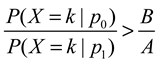
The condition for rejecting the null hypothesis () is:
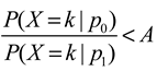
The condition for continuing sampling is:
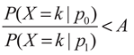
Where A and B are the upper and lower limits, calculated as:


Solving the model gives the change in the acceptance probability under different defect rates, as shown in Figure 1.
From the solution results of the changes in acceptance probability under different defect rates in Figure 1, it can be seen that with a 95% confidence level, when the sample size is large, batches with high defect rates are eventually rejected, while batches with low defect rates are ultimately accepted. For batches with defect rates of 0.12 and 0.14, when the sample size reaches around 600 to 700, the acceptance probability approaches zero, meaning that at this point the company can reject these high defect rate batches with 95% confidence. In particular, for the curve with a defect rate of 0.14, when the sample size is close to 700, its acceptance probability is significantly lower than the 95% confidence level line, indicating that the company can confirm that the defect rate has exceeded the standard and reject this batch of components. Under a 90% confidence level, for batches with lower defect rates, their acceptance probability quickly reaches the 90% confidence level line as the sample size increases. For the curve with a defect rate of 0.04, when the sample size is around 400, its acceptance probability has already exceeded the 90% confidence level line, indicating that the company can decide to accept this batch of components at that point. Similarly, for a batch with a defect rate of 0.06, when the sample size reaches 500, the acceptance probability has already exceeded the 90% confidence level. The enterprise can make the acceptance decision at this sample size, thus avoiding unnecessary additional sampling inspections. The specific sampling plan design is shown in Table 1.
From the sampling plan in Table 1, it can be seen that at a 95% confidence level, enterprises can make decisions within a relatively large sample size range (400-700). For low defect rates (such as 0.04 and 0.06), a decision to accept can be made when the sample size reaches 400-600; for high defect rates (such as 0.12 and 0.14), a decision to reject should be made when the sample size reaches 600-700. At a 90% confidence level, the sample size can be relatively reduced. The rapid acceptance strategy is suitable for batches with lower defect rates (such as 0.04 and 0.06), where a sample size between 300 and 400 is sufficient to make an acceptance decision; for batches with medium defect rates (such as 0.08 and 0.10), decisions can be made with a sample size between 400 and 500; for batches with high defect rates (such as 0.12 and 0.14), a sample size of 500–600 should lead directly to rejection.
The minimal sampling plan is as follows: at a 95% confidence level, for batches with lower defect rates, the minimum sample size between 400 and 600 is sufficient to make an acceptance decision. At a 90% confidence level, for batches with lower defect rates, the minimum sample size between 300 and 400 is sufficient to make an acceptance decision.
3. Optimisation of Spare Parts and Finished Product Inspection and Production Processes
The defect rate of the finished products is jointly influenced by the defect rates of Spare Part 1 and Spare Part 2, and even when both spare parts meet the quality standards, the finished product may still fail to meet the quality requirements due to other factors in the assembly process. Therefore, the enterprise needs to decide whether to inspect spare part 1 and 2. If inspection is required, the enterprise will incur a certain inspection cost and can eliminate defective spare parts in the process, thereby reducing the defective rate in the assembly. The inspection cost for spare part 1 and 2 can be expressed by the following formula:
If no inspection is conducted, there will be potential losses, calculated using the following formula:
Here,represent the quantity of spare part 1 and 2 respectively, represent the defective rates of spare part 1 and 2, represent the probability of being qualified, represent the loss caused by defective spare parts entering the assembly, and represent the replacement loss caused by customers returning defective finished products. If the inspection cost is less than the potential loss , choose to conduct the inspection.
The enterprise needs to decide whether to perform corresponding inspections on finished products to avoid return and exchange losses caused by substandard products entering the market. First, a cost-benefit analysis needs to be conducted. When inspecting the finished products, the inspection cost for finished products is:
Where refers to the cost of the finished product inspection, represents the quantity of the finished products, and represents the inspection cost per finished product.
When the finished products are not inspected, the potential loss is:
The enterprise needs to decide whether to disassemble the defective finished products or whether to recover the qualified components or discard the defective ones. At this point, it is necessary to conduct a cost-benefit analysis of the disassembly strategy for defective finished products. When the defective finished products are disassembled, the disassembly cost is:
Where is the disassembly cost per finished product.
When the defective finished products are disassembled, the disassembly revenue is:
Among them, represents the probability of qualified parts after disassembly, and represents the value of each recovered part. If the disassembly cost of the substandard finished products is less than the revenue, disassembly should be chosen.
When consumers return finished products that do not meet the standards, the enterprise must choose between two handling strategies: direct disposal or disassembly. If the disassembly strategy is chosen, the following two cost factors must be considered: disassembly cost and replacement loss.
Among them,represents the logistics cost during the return process, andrepresents the expected revenue from the qualified components recovered through disassembly.
Enterprises need to comprehensively calculate the costs at each stage of the entire production process to obtain the expected total cost:
Among them,is the cost of parts inspection, for which the expected cost is calculated based on whether parts inspection is selected;is the cost of finished product inspection, for which the expected replacement loss is calculated based on whether finished product inspection is selected; andis the disassembly cost, for which the profit or loss after disassembling non-conforming products is calculated based on whether disassembly is selected. The total production cost of the enterprise can be obtained using the following formula:
Among them, is the revenue from selling qualified finished products.
In order to optimise each decision step in the production process, enterprises can use dynamic programming to optimise the overall decision path. The specific formula for dynamic programming to optimise the decision path is:
Among them:is the value function of the state, representing the minimum expected cost starting from the state;is the immediate cost of taking actionin state;is the state transition probability, the probability of transitioning from stateto stateafter taking action.
There are two types of parts, and each part can be either inspected or not inspected, so there are a total of four strategy combinations for the parts. Each finished product can be either inspected or not inspected, and defective finished products can be either dismantled or not dismantled. Therefore, there are also a total of four strategy combinations for the finished products. In summary, there are 16 different strategy combinations in total, each combination representing the inspection decision of part 1 and 2, and the inspection and dismantling decisions for the finished product. As shown in Table 2 for different situations and strategies.
Table 2 presents 16 different combinations of strategies for the inspection and handling of spare parts and finished products. By combining different strategies, companies can choose the most suitable quality control plan according to specific circumstances, making trade-offs based on cost constraints, resource availability, or quality requirements. These strategies can help companies optimise quality management and resource recovery efficiency in the production process.
Figure 2 compares the total costs of the different strategies across the 16 scenarios. It can be seen that in scenarios 1-4, the situation is relatively stable, with little cost difference among the strategies. In these scenarios, companies can adopt more flexible inspection or dismantling strategies. In scenario 5, costs begin to decrease for some strategies, indicating that appropriate adjustments in strategy can effectively control costs. In scenario 6, costs rise sharply, suggesting that more precise decisions are needed, such as effective inspection and handling measures for high defect rates, with dismantling cost management being particularly critical.
Based on the comparison of total costs under different scenarios shown in Figure 2, and combined with the 16 situations encountered by the enterprise in production as given in the table, the specific solutions for the 16 situations are as follows:
Scenario 1: (1) For spare parts 1 and 2: Due to a relatively high defect rate and relatively low inspection costs, it is recommended to inspect spare parts 1 and 2 to reduce defective items entering the assembly stage; (2) For finished product inspection: The inspection cost of finished products is lower than the replacement loss, so it is recommended to inspect finished products; (3) For finished product disassembly: Disassembly cost is relatively low, and if defective finished products are detected, it is recommended to disassemble them.
Scenario 2: (1) For spare parts 1 and 2: With a high defect rate, it is recommended to inspect spare parts 1 and 2; (2) For finished product inspection: Finished product inspection cost remains relatively low, with the replacement loss the same as in Scenario 1, so finished products inspection is recommended; (3) For finished product disassembly: Same as Scenario 1, disassembly is recommended to avoid additional losses caused by defective products.
Scenario 3: (1) For spare parts 1 and 2: With relatively low inspection costs, it is recommended to continue inspecting spare parts 1 and 2; (2) For finished product inspection: Inspection cost is much higher than replacement loss, so finished product inspection is not recommended, instead go directly to market and bear the replacement loss; (3) For finished product disassembly: With relatively low disassembly costs, direct disassembly is recommended.
Scenario 4: (1) For spare parts 1 and 2: with a low defect rate and low inspection cost, it is recommended to continue inspecting the spare parts; (2) For finished product inspection: with high inspection cost and high replacement loss, it is recommended not to carry out finished product inspection and to bear the replacement loss; (3) For finished product disassembly: with relatively low disassembly cost, it is recommended to perform disassembly to reduce losses.
Scenario 5: (1) For spare parts 1 and 2: the inspection cost for spare part 1 is high, so it is not recommended to inspect spare part 1; the inspection cost for spare part 2 is low, so it is recommended to inspect spare part 2; (2) For finished product inspection: with relatively low inspection cost, it is recommended to continue finished product inspection; (3) For finished product disassembly: with relatively low disassembly cost, it is recommended to perform disassembly.
Scenario 6: (1) For spare parts 1 and 2: with low defect rate and inspection cost, it is recommended not to inspect the spare parts; (2) For finished product inspection: with low inspection cost and high replacement loss, it is recommended to carry out finished product inspection; (3) For finished product disassembly: with high disassembly cost, it is recommended to directly discard nonconforming finished products.
Output the final decision table for the above 6 scenarios, with the corresponding indicator results shown in Table 3:
As can be seen from Table 3, Scenarios 1 and 2 are suitable for production contexts that pursue high quality and low defect rates. Although inspection costs are high, they can prevent subsequent losses caused by defective products. Scenarios 3 and 4 are suitable for situations where the defect rate is relatively low and the enterprise can accept a higher defect rate. Disassembly operations can partially compensate for insufficient inspection but still carry high cost risks. Scenario 6, although saving on disassembly costs, has high replacement losses, making it suitable when the finished product quality is relatively good.
4. Optimal Production Strategies for Multiprocess and Multicomponent Combinations
The dynamic bayesian network (DBN) is an extension of the Bayesian networks used to represent stochastic processes that change over time. It establishes dependencies between states at each time step and is suitable for solving dynamic problems involving multiple stages and multiple decisions. Thus, it is possible to simulate the evolution over time of various factors in each production stage, such as the defective rates of different spare parts and finished products, inspection costs, assembly costs, and disassembly decisions, and to optimise decision-making .
To help enterprises optimise decision-making at each stage of the production process regarding key steps such as inspection, assembly, and disassembly, with the goal of minimising total cost, which mainly includes assembly cost, inspection cost, and disassembly cost. By modelling these costs, the key factors affecting the total cost can be identified, enabling the formulation of effective production and inspection decisions.
The objective function can be expressed as:
Where: is the cost of inspecting parts and finished products; is the assembly cost caused by defective products entering the assembly process; is the market replacement loss caused by not inspecting finished products; is the disassembly cost for unqualified finished products.
The fitness function is based on the negative value of the total cost, as genetic algorithms are usually applied to maximisation problems, while this problem aims to minimise costs. The fitness calculation for each individual includes the following costs:
(1) Inspection Cost: The inspection cost refers to the economic expenditure incurred for conducting inspections and tests to ensure the quality standards of parts or finished products. Such inspection activities are key measures to reduce the risk of defective products entering the assembly process and are therefore regarded as important investments to reduce losses during the assembly stage and the cost of market replacements. The inspection cost can be expressed by the following formula:
Where: refers to the cost of inspecting parts; refers to the cost of inspecting finished products; denotes the quantity of parts; indicates whether to inspect spare part .
(2) Assembly Cost:
Where: denotes the defect rate of parts ; refers to the assembly cost potentially caused by each part during the assembly process; indicates the decision variable of whether to inspect the finished products.
(3) Cost of handling defective products: If finished products are not inspected, defective products entering the market may cause replacement losses, which can be expressed as:
Where: is the defect rate of the finished product, is the defective rate of the finished products.
(4) Disassembly cost: For finished products determined to be defective through inspection, the company has the option to disassemble them to recover usable parts. The economic expenditure incurred in this process is referred to as the disassembly cost, which can be expressed as:
Where: is the disassembly fee, and is the decision variable indicating whether to disassemble the defective finished products.
The defect rate of spare parts and finished products must not exceed a certain threshold, and the sequence of inspection and assembly must meet process requirements, meaning that spare parts must be inspected or assembled first before the inspection or assembly of finished products.
Assuming that these 8192 strategy combinations are obtained by encoding multiple binary decision variables, the strategies can be represented using an appropriate number of bits. As 8192 strategies can be represented 213, therefore each strategy requires 13-bit binary encoding. By solving, the distribution of the finished product defect rates under different strategies, comparison of the finished product defect rates under different strategies, comparison of the total costs under different strategies, and the distribution of the total costs under different strategies are shown in Figure 3, Figure 4 and Figure 5, and 6 respectively.
From the distribution of the finished product defect rates under different strategies in Figure 3, it can be observed that the overall finished product defect rate shows a downward trend during the optimisation process of the genetic algorithm. In particular, in the early stage, the rapid decline in the defect rate indicates that there are strategies with high defect rates in the initial population, while as optimisation progresses, strategies with low defect rates gradually gain dominance. In actual production, enterprises can quickly reduce the defective rate of finished products through early optimisation, thereby achieving better quality control in a short time.
From the comparison of the defective rates of the finished products under different strategies in Figure 4, it can be seen that the differences in the defective rates between the strategies are significant, indicating that some strategies have considerable advantages in reducing the defective rates of the finished products. During the production process, enterprises should choose strategies with lower defective rates to ensure effective control of the finished product quality.
From the comparison of total costs under different strategies in Figure 5, it can be concluded that the choice of strategy has a significant impact on the total cost. Some strategies reduce defective rates by increasing inspection and dismantling costs, while others save funds by reducing inspection costs, which may, however, lead to higher defective rates. Enterprises should weigh costs against quality according to their own needs and choose a strategy with a lower total cost and an acceptable rate of defective products in finished goods.
From the comparison of total costs under different strategies in Figure 6, it can be seen that with the optimisation of the genetic algorithm, the initial total cost drops rapidly, indicating the existence of high-cost strategies in the initial population. As the number of generations increases, the total cost gradually converges, indicating that the algorithm [6] explored different combination strategies in the process of finding the optimal solution. Enterprises can use the optimisation process of the genetic algorithm to find an optimal production strategy that achieves an ideal balance between the total cost and the defective rate of finished goods, thereby improving production management.
Since the defective rate of spare parts 1-8 is relatively high (especially parts 1, 2, 3, and 5), it is recommended to test parts 1, 2, 3, and 5 to reduce the subsequent defective rate of the finished goods. When the inspection cost is relatively low, inspection decisions can lead to significant quality improvement. Parts 4, 6, 7, and 8: These parts have relatively high inspection costs but also a low defect rate, so in most cases the inspection can be omitted. Finished products 1 and 2: The decision to inspect finished products should be based on the balance between the cost and the defect rate shown in the chart. If the defect rate is higher than 0.75, inspection should be prioritised to avoid market losses caused by a high defect rate. For finished products found to have a high defect rate, dismantling and reusing them should be prioritised to save production costs. Especially when the total cost is high, disassembly can effectively reduce scrapping and lower costs.
A summary of the specific decision plans is shown in Table 4:
As can be seen from Table 4, for Product 1, the company may choose not to inspect due to confidence in the entire production process, while for Product 2, the choice of disassembly or scrapping is due to its higher defect rate, as further processing would result in more resource waste or negative market impact. For the selection of detecting spare parts and finished products, enterprises should continue to collect more production data and market feedback through dynamic models.
5. Defective Rate Dynamic Monitoring and Decision Optimisation
The dynamic bayesian network (DBN) is an extension of the Bayesian networks used to represent stochastic processes that change over time. It establishes dependencies between states at each time step and is suitable for solving dynamic problems involving multiple stages and multiple decisions. Thus, it is possible to simulate the evolution over time of various factors in each production stage, such as the defective rates of different spare parts and finished products, inspection costs, assembly costs, and disassembly decisions, and to optimise decision-making.
Use the sampling inspection scheme in the optimal sampling inspection to determine the initial defect rate of each component. Initialise the state variables of the dynamic Bayesian network, which represent the initial quality state of each component.
The state at each time stepd t depends on the state of the previous moment t-1 as well as the current inspection and assembly decisions:
If performs the detection, thendepends on the detection result; if no detection is performed, thendirectly inherits from. The state transition of semifinished and finished products is similar:
The status of the semifinished products depends on the status of the currently assembled components, while the status of the finished products depends on the quality of the semi-finished products and the defect rate generated during assembly.
At each moment t, decide whether to perform inspection and disassembly based on the system status . By applying Bayesian inference [1], calculate the probability of the defect rate without inspection, and based on this, decide whether to inspect or proceed directly with the assembly.
The total cost consists of the inspection, assembly, and disassembly costs at each stage, as well as the replacement loss caused by defective products entering the market.
By solving the dynamic Bayesian network model, optimal decisions for each stage (such as component inspection, assembly, etc.) can be obtained, ensuring minimisation of the total production cost while controlling the defect rate of the finished products. The model is solved using Matlab, and the corresponding defective rates are shown in Figure 7 and Figure 8.
From Figure 7, it can be seen that in all cases, the defective rate of spare part 1 fluctuates mostly around 0.1, with Condition 4 being lower, below 0.05. The defective rate of spare part 2 is relatively high in all cases, remaining between 0.2 and 0.25. The defect rate of the finished products is relatively low, usually between 0.1 and 0.15, while in Scenario 4 the defect rate is higher, nearing 0.18. As shown in Figure 8, spare parts 2, spare parts 3, and semi-finished product 2 have higher defect rates, each approaching or exceeding 0.2, while the updated defect rate of the finished products is 0.18, which is considered a medium level.
The costs under various strategies and the losses of each spare part, semifinished product, and finished product are shown in Figure 9 and Figure 10 respectively.
Figure 9 shows that the total costs of Strategies 3, 4, 5, and 6 are relatively low, indicating that these strategies are more cost-efficient choices. The total costs of Strategies 7 to 16 are significantly higher, especially Strategies 8 and 12-16, suggesting that under these strategies, the enterprises incur greater costs, possibly due to higher defect rates or higher inspection and disassembly costs. From Figure 10, it can be seen that defective losses are higher for Spare Part 2, Spare Part 3, Semi-finished Product 2, and Finished Products, indicating relatively high defect rates in these items and suggesting that particular attention should be paid to their quality control. Spare Parts 5, 7, and 8 have lower defective losses, indicating lower defect rates and hence smaller losses.
The decision plan in Table 5 shows that under different scenarios, enterprises exhibit strong flexibility in their inspection and disassembly decisions for spare parts and finished products. The choice of inspection and disassembly is based on balancing the quality of the components and finished products, the inspection costs, and the defective rates.
From Table 5, it can be seen that both Component 1 and Component 2 undergo inspection to ensure that defective components do not enter the assembly stage, thereby maximising the assurance of the finished product quality. At the same time, the finished products are inspected so that all defective products can be promptly identified and disassembled to reduce overall losses. During the disassembly process, the disassembly strategy allows qualified components from defective finished products to be reused, reducing the impact of defective rates on the total cost.
The recalculation yields the new sampling plan for Problem 2 and the new corresponding indicator results for Problem 3, as shown in Table 6 and Table 7.
Table 6 shows the inspection decisions made by the company during production based on the quality conditions of the different components and finished products. By focusing on the inspection of parts with high defect rates, enterprises can ensure the overall quality of the finished products while reducing the inspection costs. For parts that do not affect the overall quality, a no-inspection approach is chosen to optimise resource allocation. In addition, the handling plan for finished products (such as no inspection or scrapping) is optimised based on comprehensive considerations including quality and repair costs.
6. Conclusions
The contributions of this study are multifaceted, providing effective solutions for optimising quality inspection and decision-making paths in electronic product manufacturing processes and covering the following key aspects.
Advanced data analysis and inspection optimisation: This study combines hypothesis testing and sequential probability ratio test methods to deeply analyse the defect rates of different parts and proposes optimal sampling inspection schemes based on different confidence levels. This method effectively reduces the number of inspections while ensuring detection accuracy, significantly optimising the quality control process in electronic product manufacturing.
Defective rate monitoring and production efficiency improvement: By combining dynamic programming and dynamic Bayesian networks, this study provides a comprehensive optimisation plan for multi-stage production processes, enabling tne dynamic monitoring of defective rates at each stage during production. The research results indicate that using these methods can dynamically adjust production strategies, improve production efficiency, reduce production losses, and achieve more effective quality control.
Production and cost optimisation: The study uses genetic algorithms to optimise the combination problems of multiple processes and multiple components in complex production flows, identifying the optimal strategy combination that minimises total production costs. The optimised solution not only enhances the economic benefits of the production process but also reduces production waste while maintaining high product quality.
Optimal Decision-making under Resource Constraints: This study addresses issues such as component inspection and finished product disassembly in electronic product manufacturing, proposing solutions based on dynamic programming and genetic algorithms. In complex production environments, it can help enterprises balance inspection costs with market demand under limited resources, ensuring efficiency and profitability in the production process.
Recommendations for production management and supply chain optimisation: Overall, this study has made significant contributions to the fields of production management and supply chain optimisation by streamlining inspection processes, reducing defect rates, and implementing data-driven decision-making methods. These methods and research findings provide valuable insights for electronic product manufacturers seeking to improve production efficiency, reduce waste, and increase profitability in a highly competitive market.
Taken together, these contributions highlight the importance of data-driven decision-making and optimised production processes in addressing challenges in the electronic manufacturing industry, particularly in managing complex production workflows and reducing defect rates.
Author Contributions
Conceptualization, Siyuan Song and Lizhu Su; methodology, Siyuan Song and Lizhu Su; validation, Siyuan Song and Lizhu Su; formal analysis, Siyuan Song and Lizhu Su; investigation, Siyuan Song and Lizhu Su; resources, Siyuan Song and Lizhu Su; data curation, Siyuan Song and Lizhu Su; writing—original draft preparation, Siyuan Song, Lizhu Su, Jiazhe Ji, Jiarun Cui Xinyu Wang and RuiYan; writing—review and editing, Siyuan Song and Lizhu Su; visualization, Jiazhe Ji, Jiarun Cui Xinyu Wang and RuiYan; All authors have read and agreed to the published version of the manuscript.
Funding
This research received no external funding.
Data Availability Statement
Dataset is available upon request from the authors.
Acknowledgments
The authors have reviewed and edited the output and take full responsibility for the content of this publication.
Conflicts of Interest
The authors declare no conflicts of interest.
References
- You, J.; Li, M.; Guo, K.; Li, H. Integrated control policy for a multiple machines and multiple product types manufacturing system production process with uncertain fault. Processes 2020, *8*, 40. [Google Scholar] [CrossRef]
- Guo, R.; Zhong, Z.W. Assessing WEEE sustainability potential with a hybrid customer-centric forecasting framework. Sustain. Prod. Consum. 2021, *27*, 1918–1933. [Google Scholar] [CrossRef]
- Rau, H.; Budiman, S.D.; Regencia, R.C.; Salas, A. A decision model for competitive remanufacturing systems considering technology licensing and product quality strategies. J. Clean. Prod. 2019, *239*, 118070. [Google Scholar] [CrossRef]
- Li, C.L.; Nenes, G. Economic modelling and optimisation of SPRT-based quality control schemes for individual observations. Int. J. Prod. Res. 2024, *62*, 8766–8789. [Google Scholar] [CrossRef]
- Khan, M.F.; Haq, A.; Ahmed, A.; Ali, I. Multiobjective multi-product production planning problem using intuitionistic and neutrosophic fuzzy programming. IEEE Access 2021, *9*, 37466–37486. [Google Scholar] [CrossRef]
- Puttero, S.; Verna, E.; Genta, G.; Galetto, M. Impact of product family complexity on process performance in electronic component assembly. Int. J. Adv. Manuf. Technol. 2024, *132*, 2907–2922. [Google Scholar] [CrossRef]
- Siddiqui, A.; Zia, M.; Otero, P. A novel process to setup electronic products test sites based on figure of merit and machine learning. IEEE Access 2021, *9*, 80582–80602. [Google Scholar] [CrossRef]
- Zhou, J.; Liang, D.C.; Liu, Y.; Huang, T.D. Robust possibilistic programming-based three-way decision approach to product inspection strategy. Inf. Sci. 2023, *646*, 119396. [Google Scholar] [CrossRef]
- Ren, H.P.; Chen, R.; Lin, Z.J. A study of electronic product supply chain decisions considering quality control and cross-channel returns. Sustainability 2023, *15*, 6709. [Google Scholar] [CrossRef]
- Frumosu, F.D.; Khan, A.R.; Schioler, H.; Kulahci, M.; Zaki, M.; Westermann-Rasmussen, P. Cost-sensitive learning classification strategy for predicting product failures. Expert Syst. Appl. 2020, *161*, 113687. [Google Scholar] [CrossRef]
- Li, B.; Li, J.P.; Li, W.R.; Shirodkar, S.A. Demand forecasting for production planning decision-making based on the new optimised fuzzy short time-series clustering. Prod. Plan. Control 2012, *23*, 663–673. [Google Scholar] [CrossRef]
- Sarkar, B.; Saren, S. Product inspection policy for an imperfect production system with inspection errors and warranty cost. Eur. J. Oper. Res. 2016, *248*, 263–271. [Google Scholar] [CrossRef]
- He, Q.C.; Chen, Y.J. Dynamic pricing of electronic products with consumer reviews. Omega 2018, *80*, 123–134. [Google Scholar] [CrossRef]
- Pan, R.S.; Yu, J.H.; Zhao, Y.M. Many-objective optimization and decision-making method for selective assembly of complex mechanical products based on improved NSGA-III and VIKOR. Processes 2022, *10*, 373. [Google Scholar] [CrossRef]
- Bhatia, N.; Gülpinar, N.; Aydin, N. Dynamic production-pricing strategies for multi-generation products under uncertainty. Int. J. Prod. Econ. 2020, *230*, 107895. [Google Scholar] [CrossRef]
- Pan, R.J.; Zhang, Z.B.; Li, X.; Chakrabarty, K.; Gu, X.L. Black-box test-cost reduction based on bayesian network models. IEEE Trans. Comput.-Aided Des. Integr. Circuits Syst. 2021, *40*, 386–399. [Google Scholar] [CrossRef]
- Falih, A.; Shammari, A. Hybrid constrained permutation algorithm and genetic algorithm for process planning problem. J. Intell. Manuf. 2020, *31*, 1079–1099. [Google Scholar] [CrossRef]
- Tamás, P.; Tollár, S.; Illés, B.; Bányai, T.; Tóth, A.B.; Skapinyecz, R. Decision support simulation method for process improvement of electronic product testing systems. Sustainability 2020, *12*, 5639. [Google Scholar] [CrossRef]
- Al-Azzawi, D.S. Evaluation of genetic algorithm optimization in machine learning. J. Inf. Sci. Eng. 2020, *36*, 231–241. [Google Scholar]
- Ren, L.; Meng, Z.H.; Wang, X.K.; Zhang, L.; Yang, L.T. A data-driven approach of product quality prediction for complex production systems. IEEE Trans. Ind. Inform. 2021, *17*, 6457–6465. [Google Scholar] [CrossRef]
- Che, Z.H. Pricing strategy and reserved capacity plan based on product life cycle and production function on LCD TV manufacturer. Expert Syst. Appl. 2009, *36*, 2048–2061. [Google Scholar] [CrossRef]
- Yu, C.M.; Chen, K.S.; Hsu, T.H. Confidence-interval-based fuzzy testing for the lifetime performance index of electronic product. Mathematics 2022, *10*, 140. [Google Scholar] [CrossRef]
- Talay, I.; Özdemir-Akyıldırım, Ö. Optimal procurement and production planning for multi-product multi-stage production under yield uncertainty. Eur. J. Oper. Res. 2019, *275*, 536–551. [Google Scholar] [CrossRef]
- Chiang, T.A.; Che, Z.H.; Wang, T.W.; Chen, J.H. Demand-oriented multi-objective planning method for electronic product technology development. Appl. Math. Model. 2016, *40*, 3620–3634. [Google Scholar] [CrossRef]
- Fathian, M.; Sadjadi, S.J.; Sajadi, S. Optimal pricing model for electronic products. Comput. Ind. Eng. 2009, *56*, 255–259. [Google Scholar] [CrossRef]
Figure 1.
Change in acceptance probability under different defect rates.
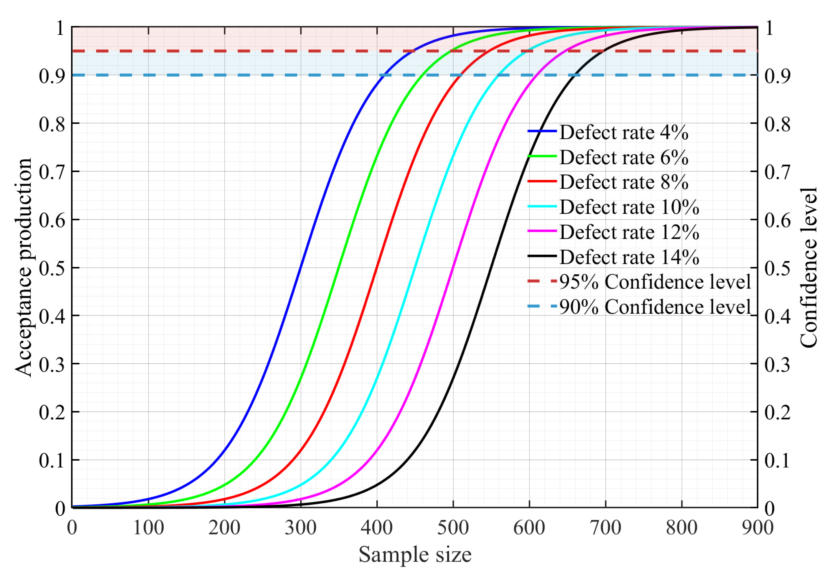
Figure 2.
Comparison of total costs under different scenarios and strategies.
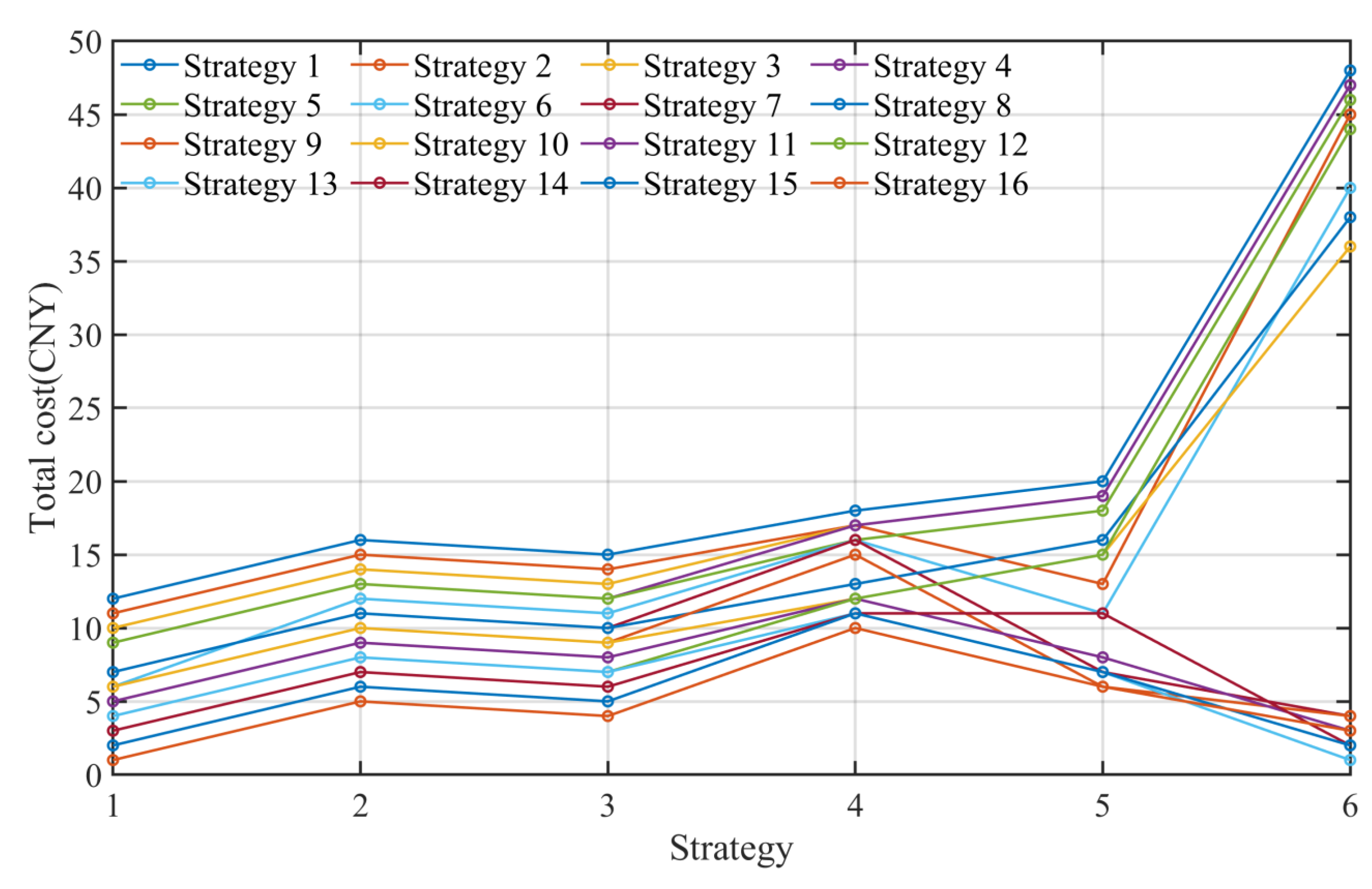
Figure 3.
Distribution of the finished product defect rate under different strategies.
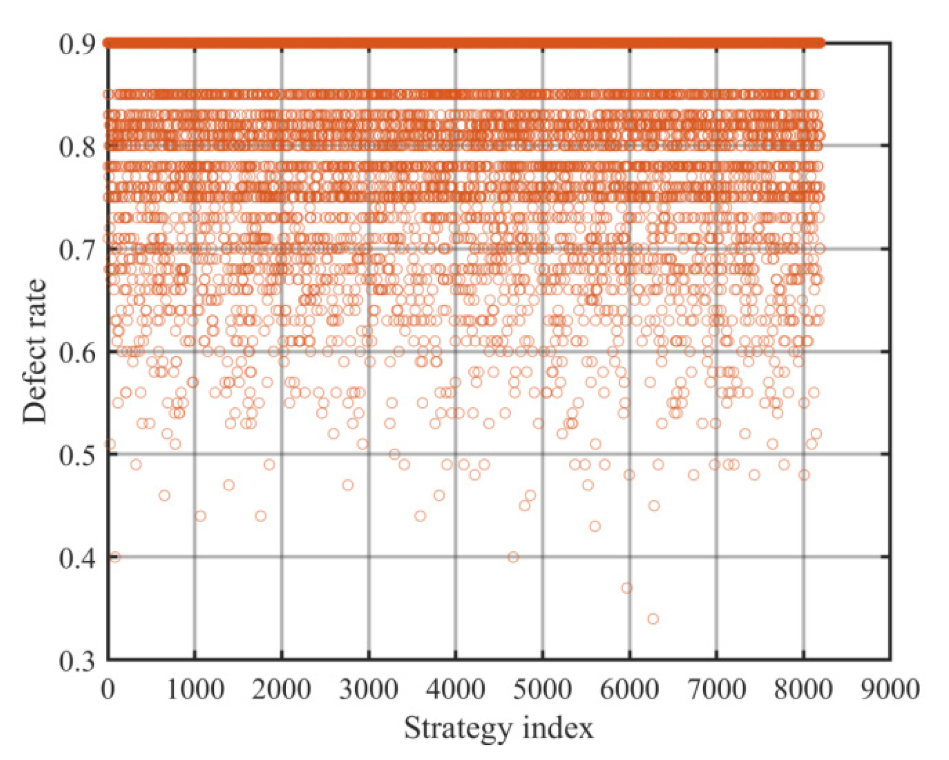
Figure 4.
Comparison of the finished product defect rates under different strategies.
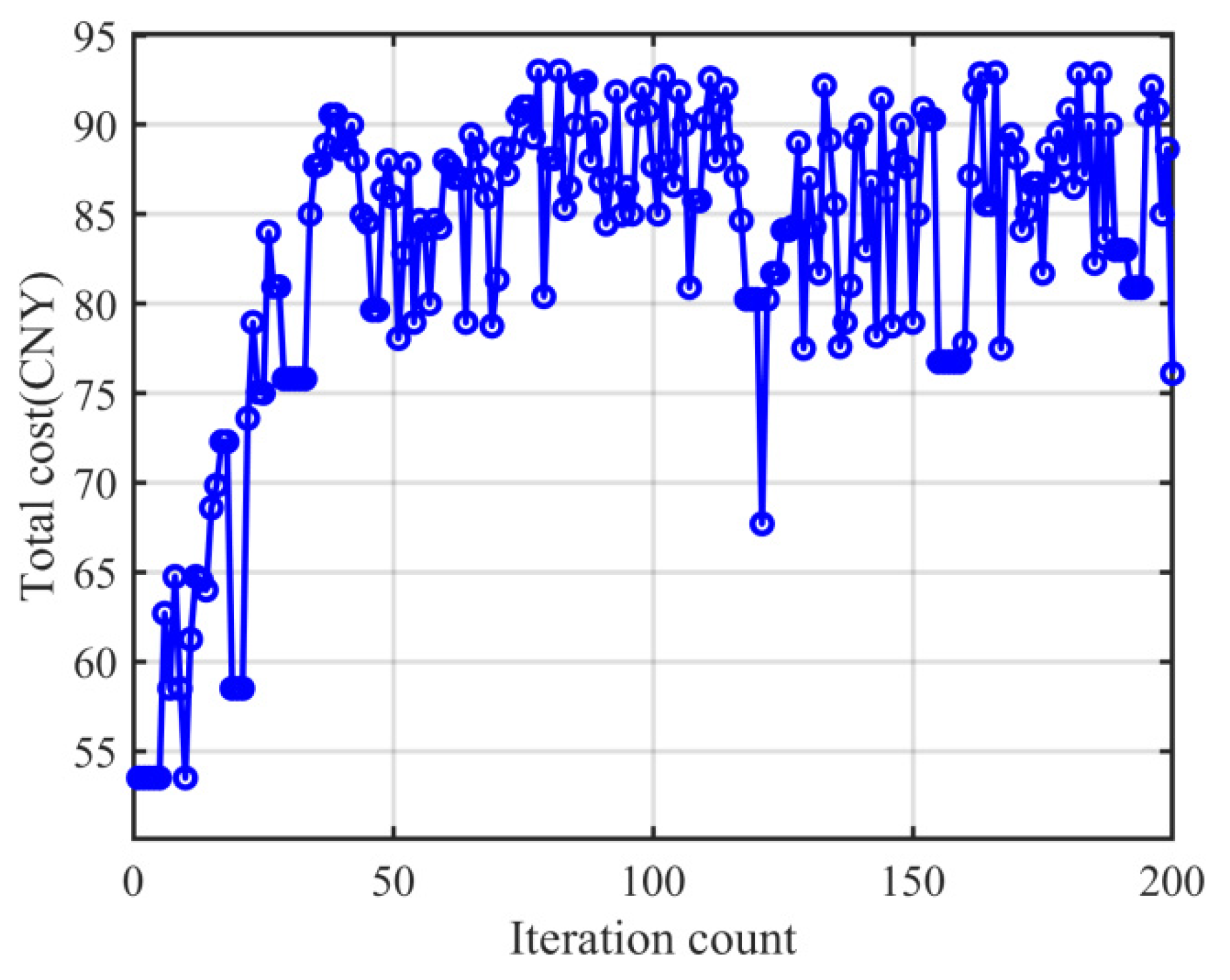
Figure 5.
Comparison of total cost under different strategies.
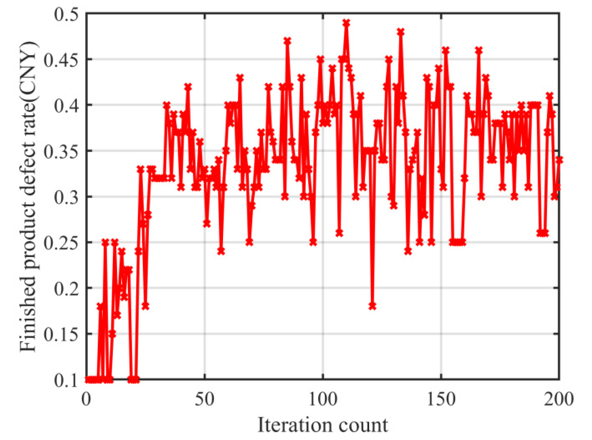
Figure 6.
Distribution of total cost under different strategies.
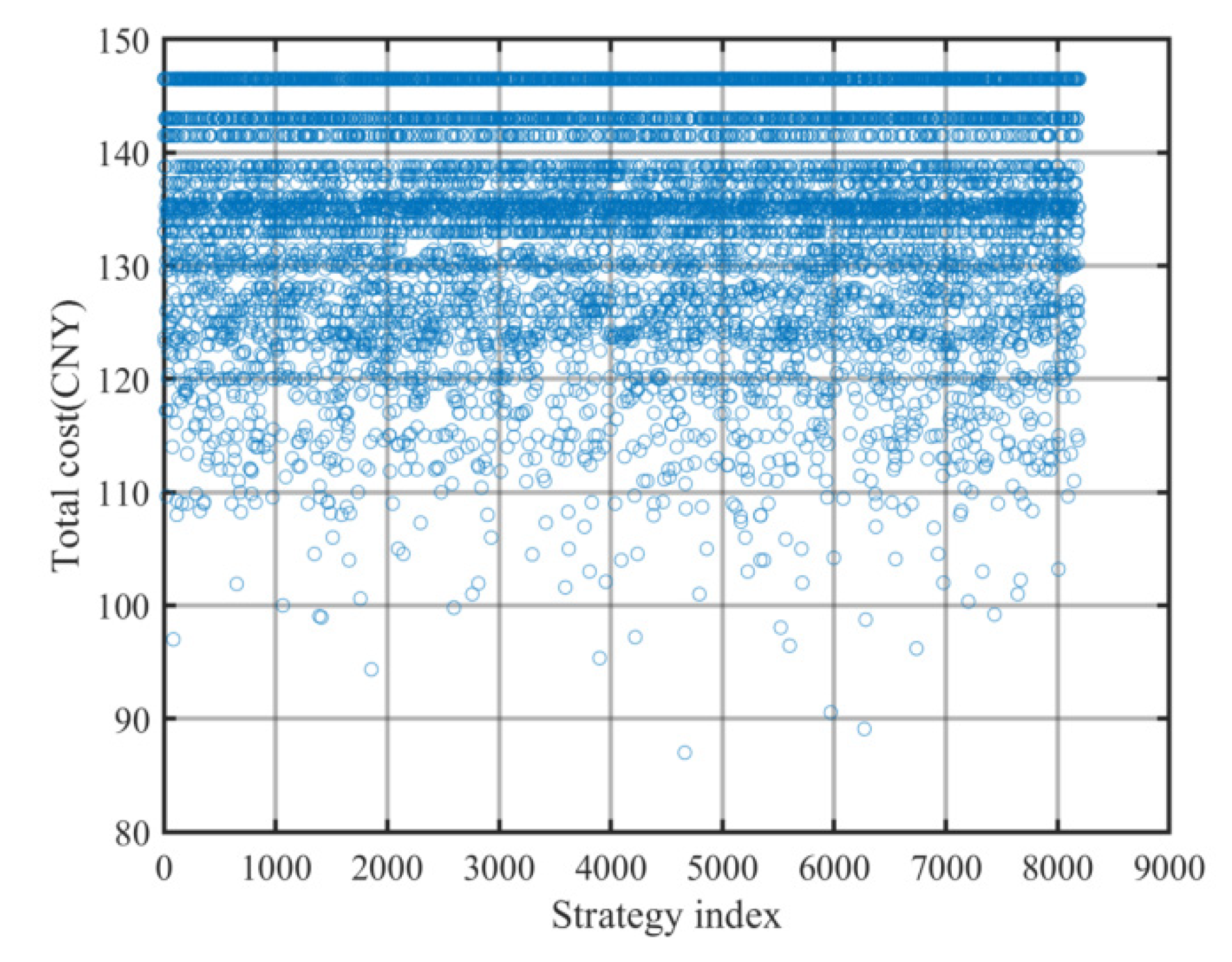
Figure 7.
Updated defective rates of spare parts and finished products under various conditions.
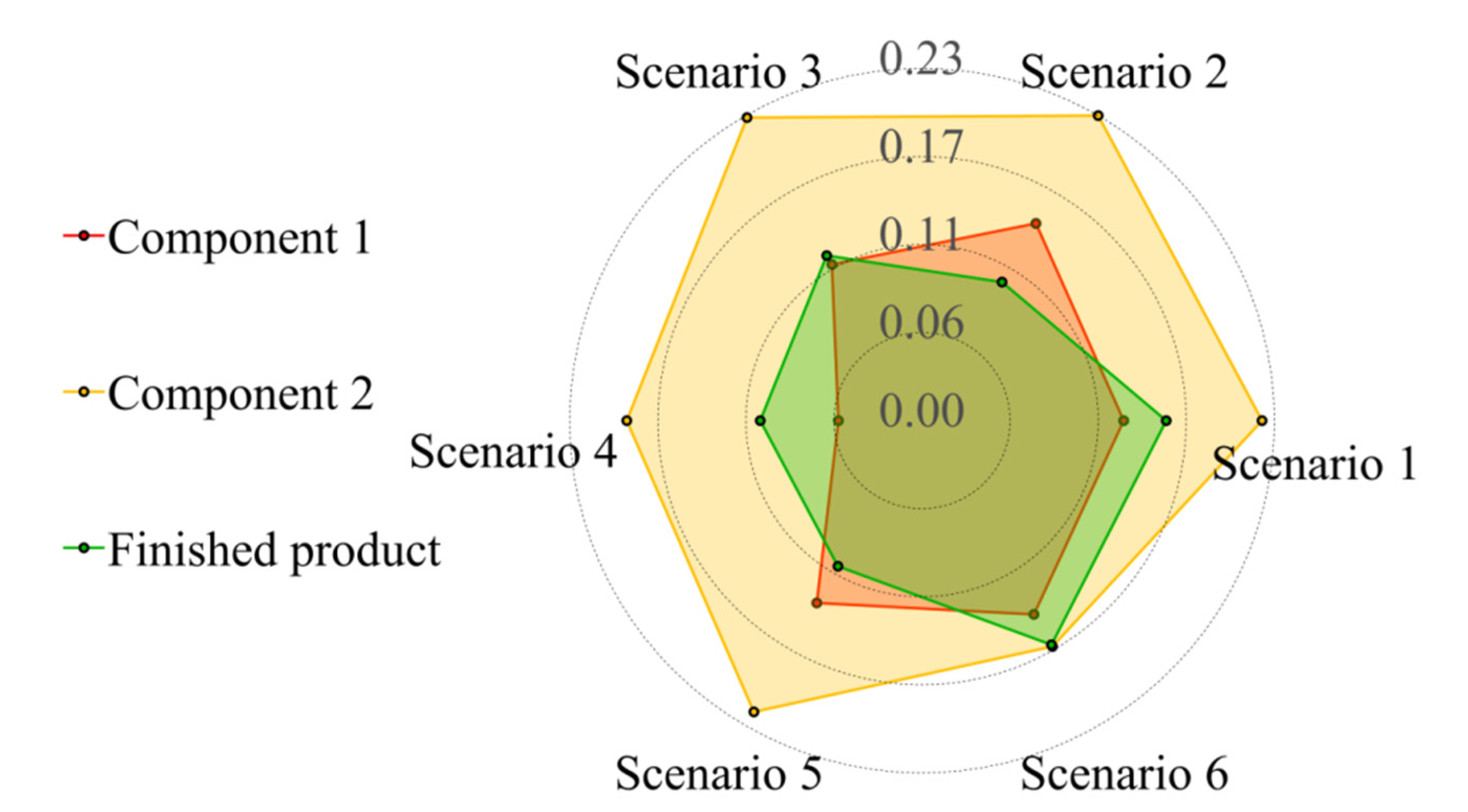
Figure 8.
Updated defective rates of spare parts, semifinished products, and finished products.
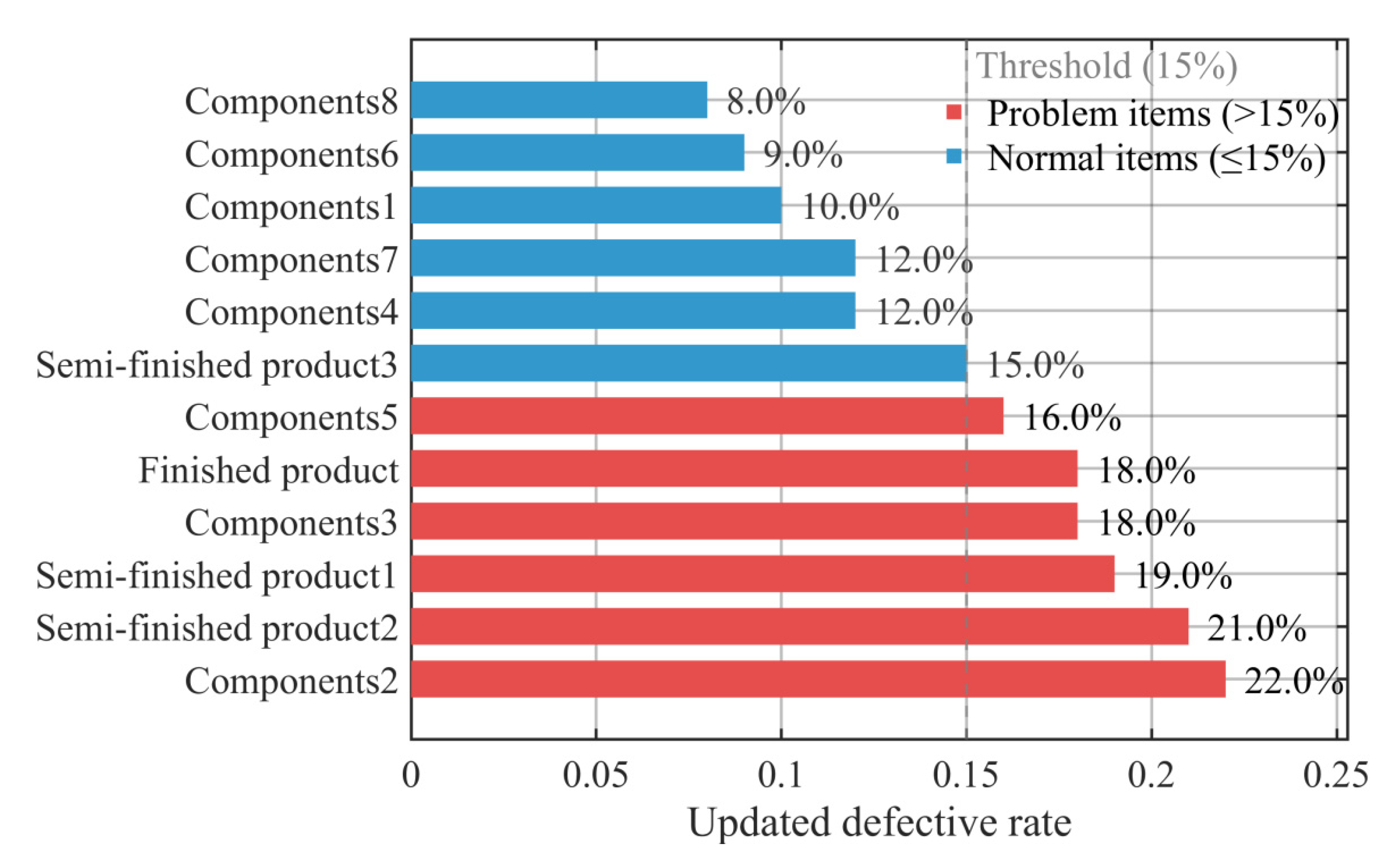
Figure 9.
Costs under Various Strategies.
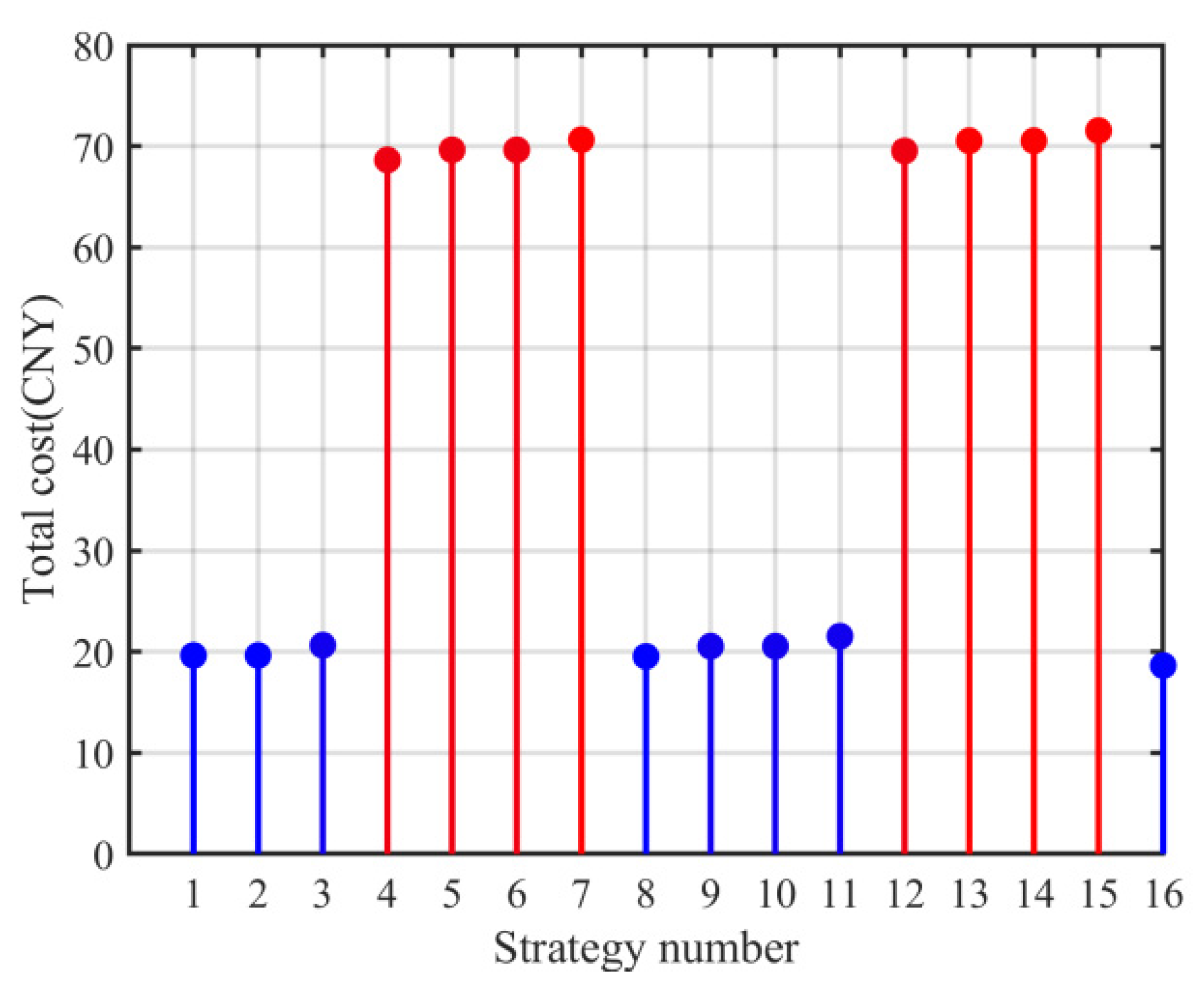
Figure 10.
Updated Defect Rates of Spare Parts, Semi-Finished Products, and Finished Products.
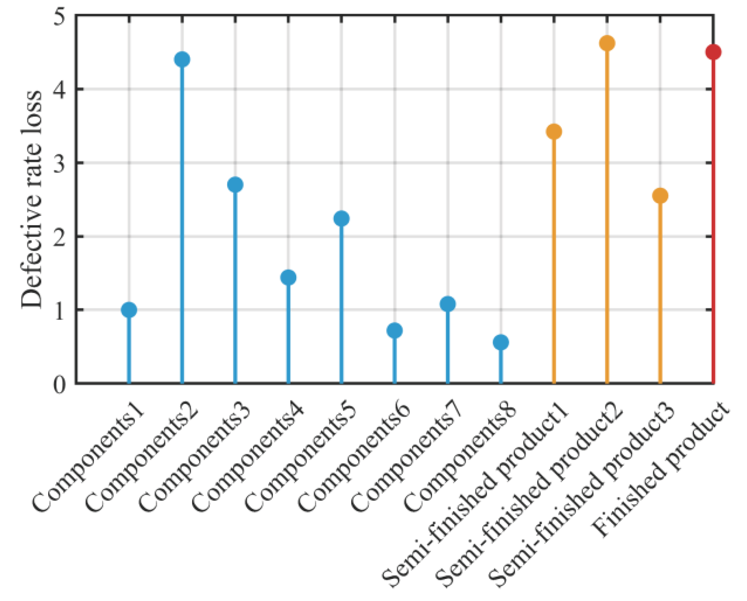

Table 1.
Sampling plan.
| Confidence level | Defective rate | Sampling strategy | Recommended sample size range | Inspection results and decisions |
|---|---|---|---|---|
| 95% | 0.04,0.06,0.08,0.10 | Dynamic Inspection Strategy | Sample size reaches 400-600 | For batches with a defect rate of 0.10 or lower, make the final decision when the sample size reaches 600; if it is below 600, the batch can be accepted. |
| 95% | 0.12, 0.14 | Dynamic Inspection Strategy | Sample size reaches 600-700 | For batches with a high defect rate, make a rejection decision when the sample size reaches 600-700; reject these batches if the sample size exceeds 700. |
| 90% | 0.04, 0.06 | Rapid Acceptance Strategy |
Sample size reaches 300-400 | For batches with a low defect rate, acceptance can be granted when the sample size reaches 300-400. |
| 90% | 0.08, 0.10 | Stepwise Inspection Strategy | Sample size reaches 400-500 | For batches with a medium defect rate, a decision to accept can be made when the sample size reaches 400-500. |
| 90% | 0.12, 0.14 | Dynamic Inspection Strategy | Sample size of 500-600 | For batches with a high defect rate, the batch should be rejected when the sample size reaches 500-600 to avoid unnecessary subsequent losses. |
Table 2.
Different Situations and Strategies.
| Strategy | Inspect spare part 1 | Inspect spare part 2 | Inspect the finished product | Dismantle the non-conforming finished product |
| 1 | Inspection | Inspection | Inspection | Disassembly |
| 2 | Inspection | Inspection | Inspection | Do not dismantle |
| 3 | Inspection | Inspection | Do not inspect | Disassembly |
| 4 | Inspection | Inspection | Do not inspect | Do not dismantle |
| 5 | Inspection | Do not inspect | Inspection | Disassembly |
| 6 | Inspection | Do not inspect | Inspection | Do not dismantle |
| 7 | Inspection | Do not inspect | Do not inspect | Disassembly |
| 8 | Inspection | Do not inspect | Do not inspect | Do not dismantle |
| 9 | Do not inspect | Inspection | Inspection | Disassembly |
| 10 | Do not inspect | Inspection | Inspection | Do not dismantle |
| 11 | Do not inspect | Inspection | Do not inspect | Disassembly |
| 12 | Do not inspect | Inspection | Do not inspect | Do not dismantle |
| 13 | Do not inspect | Do not inspect | Inspection | Disassembly |
| 14 | Do not inspect | Do not inspect | Inspection | Do not dismantle |
| 15 | Do not inspect | Do not inspect | Do not inspect | Disassembly |
| 16 | Do not inspect | Do not inspect | Do not inspect | Do not dismantle |
Table 3.
Corresponding indicator results.
| Situation | Spare part 1 | Spare part 2 | Finished roduct inspection | Finished product disassembly |
|---|---|---|---|---|
| Situation 1 | Inspection | Inspection | Inspection | Disassembly |
| Situation 2 | Inspection | Inspection | Inspection | Disassembly |
| Situation 3 | Inspection | Inspection | Do not inspect | Disassembly |
| Situation 4 | Inspection | Inspection | Do not inspect | Disassembly |
| Situation 5 | Do not inspect | Inspection | Inspection | Disassembly |
| Situation 6 | Do not inspect | Inspection | Inspection | Do not dismantle |
Table 4.
Specific decision plans.
| Item | Detection status | Item | Detection status |
| Spare part 1 | Inspection | Spare part 6 | Do not inspect |
| Spare part 2 | Inspection | Spare part 7 | Do not inspect |
| Spare part 3 | Inspection | Spare part 8 | Do not inspect |
| Spare part 4 | Do not inspect | Finished product 1 | Do not inspect |
| Spare part 5 | Inspection | Finished product 2 | Scrap or disassemble |
Table 5.
New specific decision plan for Problem 2.
| Situation | Spare part 1 | Spare part 2 | Finished product inspection | Finished product disassembly |
| Situation 1 | Inspection | Inspection | Inspection | Disassembly |
| Situation 2 | Inspection | Inspection | Inspection | Do not dismantle |
| Situation 3 | Do not inspect | Inspection | Do not inspect | Disassembly |
| Situation 4 | Inspection | Inspection | Do not inspect | Do not dismantle |
| Situation 5 | Do not inspect | Inspection | Inspection | Disassembly |
| Situation 6 | Do not inspect | Do not inspect | Inspection | Do not dismantle |
Table 6.
Specific new decision plan for Question 3.
| Item | Detection status |
|---|---|
| Spare part 1 | Inspection |
| Spare part 2 | Inspection |
| Spare part 3 | Inspection |
| Spare part 4 | Do not inspect |
| Spare part 5 | Inspection |
| Spare part 6 | Do not inspect |
| Spare part 7 | Do not inspect |
| Spare part 8 | Do not inspect |
| Finished product 1 | Do not inspect |
| Finished product 2 | Scrap or disassemble |
Disclaimer/Publisher’s Note: The statements, opinions and data contained in all publications are solely those of the individual author(s) and contributor(s) and not of MDPI and/or the editor(s). MDPI and/or the editor(s) disclaim responsibility for any injury to people or property resulting from any ideas, methods, instructions or products referred to in the content. |
© 2026 by the authors. Licensee MDPI, Basel, Switzerland. This article is an open access article distributed under the terms and conditions of the Creative Commons Attribution (CC BY) license.
Copyright: This open access article is published under a Creative Commons CC BY 4.0 license, which permit the free download, distribution, and reuse, provided that the author and preprint are cited in any reuse.


