Submitted:
19 December 2025
Posted:
22 December 2025
You are already at the latest version
Abstract
Drone localization is essential for various purposes such as navigation, autonomous flight, and object tracking. However, this task is challenging when satellite signals are unavailable. This paper addresses vision-only localization of flying drones through op-timal window velocity fusion. Multiple optimal windows are derived from a piecewise linear regression (segment) model of the image-to-real world conversion function. Each window serves as a template to estimate the drone's instantaneous velocity. The multiple velocities obtained from multiple optimal windows are integrated by two fusion rules: one is a weighted average for lateral velocity, and the other is a winner-take-all decision for longitudinal velocity. In the experiments, a drone performed a total of six short-range (about 800 m to 2 km) and high maneuvering flights in rural and urban areas. Four flights in rural areas consist of a forward-backward straight flight, a forward-backward zigzag flight (a snake path), a square path with three banked turns, and a free flight that includes both banked turns and zigzags. Two flights in urban areas are a straight outbound flight and a forward-backward straight flight. The performance was evaluated through the root mean squared error (RMSE) and drift error of the ground-truth trajectory and the rig-id-body rotated vision-only trajectory. The proposed image-based method has been shown to achieve flight errors of a few meters to tens of meters, which corresponds to around 3% of the flight length.
Keywords:
vision-only drone localization
; image–position conversion
; template matching
; optimal windows
; velocity fusion
1. Introduction
The applications of unmanned aerial vehicles (UAVs) have expanded dramatically [1,2,3]. It is crucial to determine drones’ position to perform high-level tasks. Drones typically estimate their position through an integration of external sensors, such as global positioning system (GPS) and internal sensors such as inertial measurement units (IMUs) [4,5].
Accurate localization is very challenging where GPS signals are not available [5]. Without absolute position reference, drones must rely on alternative sensing methods to infer their positions, often requiring additional onboard sensing or external infrastructure [6,7]. One prominent solution to this problem is a visual-inertial odometry system that fuses data from an inertial measurement unit (IMU) and a camera [8,9,10].
Vision-based localization offers the advantages of low cost, light weight, passive sensing, and multi-functionality. One of vision-based approaches is template-based method which localize drones by matching the current image against a pre-stored template. Object motion can be tracked by matching a template between consecutive frames. The classical template matching is well-suited for estimating small translational displacements between frames when lighting is stable and there are no rotational or scale changes [11]. Normally, template selection has been scene or object dependent, thus incorrect template updates can lead to accumulated errors that degrade performance [12]. A robust illumination-invariant localization algorithm is proposed for UAV navigation [13]. Fourier-based image phase correlation was adopted to estimate absolute velocity estimation of UAV [14]. In [15], a multi-region scene matching-based method is proposed for automated navigation of UAV. Various matching techniques are surveyed for UAV navigation in [16]. Scene-independent template matching using optimal windows were proposed in [17].
This paper addresses vision-only localization of drones for short-range and high maneuvering flights. When the camera is tilted downward to the ground and located at a specific altitude, the pixel coordinates can be converted into real-world coordinates by a ray optics-based conversion function [18,19]. However, this image-to-position conversion generates non-uniform spacing in the real coordinate system. The optimal windows were proposed to overcome this non-uniform spacing in [17]. A piecewise linear regression (segment) model [20,21] determines the breakpoints of the optimal window. The piecewise linear regression model minimizes the total least-square errors over all linear segments that approximate the conversion function. In consequence, the optimal window divides a frame into several non-overlapping templates. Each template is matched between frames by minimizing the sum of normalized squared differences [22]. In [17], this technique combined with a state estimator achieves errors of several meters on very short-range flights.
In the paper, this optimal window template matching technique is significantly improved by the fusion of velocities. Two fusion rules are contrived considering the minimum detectable velocity as the velocity resolution: weighted averaging for the lateral velocity and winner-take-all decision for the longitudinal velocity. Additionally, a zero-order hold scheme was applied to reduce the high computational burden of template matching.
In the experiments, a multirotor drone (DJI Enterprise Advanced [23]) performed short-range flights (800 m to 2 km) with high maneuverings in rural and urban areas. In rural areas, four paths consists of a straight-forward-backward flight, a zigzag forward-backward flight (snake path), a squared path with three banked turns, and a free flight including both banked turns and zigzags. In urban areas, two paths are a straight outbound flight and a straight-forward-backward flight. No yaw-only rotation (flat turn) is included in the flight. The drone starts from a stable hovering state, accelerates, and flies as fast as possible while maintaining an altitude of 40 meters and tilting the camera at a 60-degree angle.
To evaluate performance, a ground-truth trajectory is generated from GPS signals. Since the ground-truth trajectory has a different coordinate system than the vision-only trajectory, a rigid body rotation is applied to the vision-only trajectory to align one trajectory with the other. The root mean square error (RMSE) and drift error are calculated at three intermediate points and one end point. It will be shown that the proposed method achieved an error range of a few meters to tens of meters after flight. Figure 1 shows a block diagram of the proposed method.
The contributions of this study are as follows: (1) The process of converting images into real-world coordinates has been improved. This allows for more precise analysis of velocity resolution. (2) Multiple velocities obtained from multiple template matching are fused based on velocity resolution. Two fusion rules are proposed for lateral and longitudinal velocities, respectively. (3) The robustness of the system was verified through high maneuvering flights. Furthermore, system performance was verified by comparing it with the ground-truth obtained from GPS signals.
The rest of this paper is organized as follows: the optimal window template matching are presented in Section 2. The velocity fusion rules and performance evaluation are described in Section 3. Section 4 demonstrates experimental results. Discussion and conclusions follow in Section 5 and Section 6, respectively.
2. Optimal Windows for Template Matching
This section describes how the optimal windows are derived from the improved image-to-position conversion.
2.1. Improved Image-to-Position Conversion
The image-to-position conversion [17,19] applies trigonometry to compute real-world coordinates from pixel coordinates when the camera’s angular field of view (AFOV), elevation, and tilt angles are known. It is assumed that the camera rotates only around the pitch axis and that the ground is flat. The improved conversion function is as follows
where W and H are the image sizes in horizontal and vertical directions, respectively, h is the altitude of the drone or the elevation of the camera, and are the AFOV in the horizontal and vertical directions, respectively, and is the tilt angle of the camera.
Figure 2a,b visualizes the coordinate conversion function in horizontal and vertical directions, respectively: W and H are set to 3840 and 2160 pixels, respectively; and are set to 68° and 42°, respectively; h is set to 40 m; is set to 60°. In Figure 2a, eight non-linear conversion functions in the horizontal direction are shown varying the vertical index j from 1 to 2101 by 300-pixel intervals. In [17], was approximated by which is represented by only one conversion function in the horizontal direction. Figure 2b shows that the nonlinearity increases rapidly in the vertical direction, resulting in non-uniform spacing in the real coordinate system.
2.2. Optimal Windows
The vertical conversion function in Figure 2b is approximated by a piecewise linear regression model. In this model, multiple linear segments approximate the nonlinear curve. Several linear segments minimize the sum of the least square errors of the separate linear regression as follows:
where are break points for segments, and and are equal to 0 and the image size in the vertical direction, respectively, and and are the coefficients of the n-th linear regression line [20,21]. It is noted that is equal to the number of windows. The number of windows can be determined heuristically; too many windows, equivalently too few sampling points (pixels) in one window, can lead to inaccurate matching, whereas too few windows cannot compensate for the uneven spacing of the nonlinear conversion function. In the experiments, the frame was cropped by 90 pixels near the edges to remove distortions that might occur during image capture, thus optimal windows tiled in an area of 3660 × 1800 pixels. The n-th window has the size of 3660 × pixels. Figure 3 shows three piecewise linear segment models when =10, 12, 15. Figure 4 shows the corresponding optimal windows to Figure 3 in a sample frame. Total sum of squared errors which are minimized in Equation (3) are 55.3, 26.85, and 11.11.
The computational complexity of exhaustively searching all possible piecewise linear models grows exponentially with the number of segments. Dynamic programming [24,25] efficiently determines the optimal linear segments while significantly reducing computational burden. This approach first precomputes the least-squares fitting error for all candidate line segments. It then determines the optimal segment solution when n = 2. During this step, all possible least partial sum of squared errors for two-segments are calculated at . Then n is increased by one, the optimal solution for n segments are calculated using the least partial sum of squared errors obtained from the previous step. This process continues until n reaches .
The minimum detectable velocities at pixel (i, j) are calculated as and in the horizontal and vertical directions, respectively. Figure 5 shows the minimum detectable velocity when T =1/30 sec and . The j values in Figure 5a are the center of 12 optimal windows in the vertical direction in Figure 4b. The minimum detectable velocity increases rapidly in the vertical direction as shown in Figure 5b.
3. Velocity Fusion and Performance Evaluation
This section describes how to fuse the velocities of multiple optimal windows, and a zero-order hold scheme to reduce the matching counts. Performance evaluation using GPS signals is also presented at the end of the section.
3.1. Velocity Fusion
The minimum detectable velocity shown in Figure 5 represents the highest velocity resolution of each window. Assuming small window displacement between consecutive frames, the minimum detectable velocity can be considered the velocity resolution of that window. The weight on each window is calcualted based on its resolution as
where and are the variance of velocity of the n-th optimal window, in the horizontal and vertical directions, respectively, and and are the velocity resolution of the n-th window, in the horizontal and vertical directions, respectively. Assuming the uniform distribution, the variance is obtained from the resolution as and The lateral (sideways) velocities are fused by a weighted average as follows
where is the lateral velocity obtained from the n-th optimal window template matching between k and k+1 frames, and K is the number of frames. Equation (6) is the weighted least-squares estimator and the maximum likelihood estimator with zero-mean and uncorrelated Gaussian noise [26,27]. The resolution of the longitudinal velocities are drastically changed as shown in Figure 5b. Therefore, the winner-take-all strategy is adopted for the fusion of the longitudinal velocities as
where is the longitudinal velocity obtained from the n-th optimal window template matching between k and k+1 frames. This winner-take-all decision rule is meaningful when the best resolution is significantly better than others [28].
3.2. Traejctory Generation
The vision-only trajectory is formed as
where , t denotes matrix transpose, and is initialized to the zero vector. When the zero-order hold scheme is applied, the fused velocity is replaced by as follows:
where is the number of frames before the next frame matching occurs; thus, the frame-matching speed becomes frame rate (frame capture speed) divided by M.
3.3. Perofrmance Evaluation
The ground turth trajectories are obtained from GPS signals (latitude and longitude). The vision-only trajectory has a different coordinate system than the GPS coordinate system except for a common origin. Therefore, it is assumed that the vision-only trajectory is a rigid body rotated to the ground-truth trajectory as
where is the gournd truth trajectory at frame k; the initial location is also set to the zero vector; is the counterclockwise angle from the vision-only trajectory to the ground-truth trajejctory when the frame number of the trajecoty is l. The optimal rotation angle that aligns two trajectories in the least sqaure sense is obtained as [29,30]:
where is a singular value decomposition of the cross-covariance matrix , and It is noted that varies with the trajectory frame number l. The RMSE and drift error are defined, respectively, as
The RMSE error evaluates the accuracy for the entire trajectory, whereas the drift error measures the accuracy at a point. In the experiments, RMSE and drift errors are caluated at three intermediate and one end points
4. Results
4.1. Flight Paths
A multi-rotor drone (DJI Mavic Enterprise Advanced) [23] flew along six different paths in rural and urban areas. All videos were captured at 30 frame per second (FPS) with a frame size of 3840 × 2160 pixels. The altitude of the drone was maintained at 40 m, and the camera tilt angle was set to 60 degrees. The AFOV was assumed to be 68° and 42° in the horizontal and vertical directions, respectively. Figure 6 shows the ground-truth trajectories of six flight paths (Path 1 to 6) obtained from GPS signals. The starting point is marked 'O', three intermediate points or waypoints are marked 'A', 'B', 'C', and the end point is marked 'D'. Figures 6a-6d show four flight paths (Path 1 to 4) in rural areas, while Figure 6e and Figure 6f show two flight paths (Path 5 to 6) in urban areas. Rural areas are mostly flat and simple agricultural land. Urban areas, on the other hand, have complex and irregular terrain due to various artificial structures. Figure 6a and Figure 6b show a forward-backward straight path and a forward-backward zigzag path, respectively. Figure 6c is a squared path with three banked turns. Figure 6d is a free path with multiple banked turns and zigzags. Figure 6e and Figure 6f are an outbound straight path and a forward-backward straight path, respectively. No flat turn (yaw-only rotation) was included for all paths. In all flights, the drone starts from a stationary hovering state and accelerates to fly at its highest possible speed. For the forward–backward flight, an abrupt joystick reversal causes the drone to decelerate, stop, and move in the opposite direction.
Figure 7a–f show video frames when the drone passes points O, A, B, C, and D in six paths, respectively.
Table 1 shows the frame number and the ground-truth trajectory length of Paths 1 to 6. The shortest length is Path 5, at 810.99 m, and the longest length is Path 1, at 2066.7 m.
4.2. Vision-Only Rotated Trajectories
Figure 8 shows the vision-only trajectory aligned with the ground-truth trajectory. This alignment is necessary because the vision-only trajectory have a different coordinate system than the GPS trajectory. Alignment is achieved through rigid body rotation of the vision-only trajectory, as shown in Equations (11)-(14).
Figure 9 shows the ground-truth velocity obtained from the ground-truth trajectory and the vision-only rigid-body rotated velocities. The ground-truth velocity is calculated as the average velocity of the forward and backward velocities over one second. As shown in Figure 9, large errors often appears at high velocities. A few outliers were observed in the vision-only velocities. These isolated outliers can be removed using a robust statistical tool such as the Hampel filter [31], but the performance improvement was found to be minimal.
Table 2 shows the RMSE and drift error of six paths at Points A, B, C, D, and average. The RMSE error evaluates accuracy over the flight, while the drift error measures accuracy at each point. The average RMSE error ranges from 7.17 to 13.88 m, and the average drift error ranges from 9.44 to 20.25 m for six paths. The RMSE and drift errors at the end point range from 9.88 to 24.89 m and from 5.92 to 42.47 m, respectively. In terms of percentage, the worst RMSE and drift error at the end point were approximately 2.02% and 3.27%, respectively, on path 4.
4.3. Effects of Zero-Order Hold Scheme
Figure 10 shows the RMSE and drift errors for the end point and the average RMSE and drift errors when the zero-order hold scheme is applied. The frame matching rate varies from every frame (30 FPS) to one frame per second (1 FPS). The lower frame matching rate reduces the computational burden. Performance degraded in Paths 1, 2, and 5 as the frame matching rate decreased, but remained relatively stable in Paths 3, 4 and 6.
A total of 12 Supplementary Files are available online. Six MP4 videos for the flight and their corresponding GPS files (captions).
5. Discussion
The optimal window aims to ensure a uniform spacing in the real-world coordinate system. The number of optimal windows was set to 12, then the same number of velocities were obtained through template matching. These velocities were fused with two different fusion rules: weighted averaging for the lateral velocity and winner-take-all decision for the longitudinal velocity. Sideways flight produced more errors than longitudinal flight. Most errors appeared in the form of biases that were proportional to speed and in the opposite direction to the velocity. Several factors degraded the performance; the tilting caused by the drone’s thrust was ignored and the camera’s AFOV was set approximately. More precisely adjusting these approximations can improve performance. Additionally, the ground was assumed to be flat, which was more appropriate for high-altitude drones. This limitation could be alleviated through a practical post-processing solution [15]. Alternative solutions to overcome this limitation remain a topic for future research.
The zero-order hold scheme reduces computational complexity by a factor of several tens. However, slower frame matching can cause more errors.
6. Conclusions
This vision-only technique allows drones to estimate their location using only visual sensors. A novel frame-to-frame template-matching technique was significantly improved in the paper. The optimal window is derived from a piecewise linear regression model that linearizes the nonlinear image-to-real world conversion function. The optimal window template is scene-independent and requires no additional processes to update.
Multiple velocities are fused based on the minimum detectable velocity. The RMSE and drift error have been shown to range from several meters to a few tens of meters for around 800 m to 2 km length high maneuvering flights.
The technique supports a wide range of applications spanning commercial and industrial tasks as well as military missions. The flight range could be further extended, a topic of future research. Thermal imaging cameras [32] could be used in environments with no illumination, a possibility also being explored in future research.
Supplementary Materials
The following are available online at https://doi.org/10.5281/zenodo.17990832 accessed on 20 December 2025, Movies of flights for 6 paths: Path1.mp4, Path2.mp4, Path3.mp4, Path4.mp4, Path5.mp4, Path6.mp4, and corresponding GPS caption files: Path1.srt, Path2.srt, Path3.srt, Path4.srt, Path5.srt, Path6.srt.
Funding
This research was supported by a Daegu University Research Grant 2025.
Data Availability Statement
Data are contained within the article and Supplementary Materials.
Acknowledgments
The author would like to thank Kim, Jong-Ha for his guiding in the city of Andong for drone flights.
References
- Osmani, K.; Schulz, D. Comprehensive Investigation of Unmanned Aerial Vehicles (UAVs): An In-Depth Analysis of Avionics Systems. Sensors 2024, 24, 3064. [Google Scholar] [CrossRef]
- Kumar, P.; Pal, K.; Govil, M.C.; Choudhary, A. Comprehensive Review of Path Planning Techniques for Unmanned Aerial Vehicles (UAVs). ACM Comput. Surv. 2025, 58, 1–44. [Google Scholar] [CrossRef]
- Bany Abdelnabi, A.A.; Rabadi, G. Human Detection from Unmanned Aerial Vehicles’ Images for Search and Rescue Missions: A State-of-the-Art Review. IEEE Access 2024, 12, 152009–152035. [Google Scholar] [CrossRef]
- Ye, X.; Song, F.; Zhang, Z.; Zeng, Q. A Review of Small UAV Navigation System Based on Multisource Sensor Fusion. IEEE Sens. J. 2023, 23, 18926–18948. [Google Scholar] [CrossRef]
- Bhatti, U.I.; Ochieng, W.Y. Failure Modes and Models for Integrated GPS/INS Systems. J. Navig. 2007, 60, 327–348. [Google Scholar] [CrossRef]
- Alghamdi, S.; Alahmari, S.; Yonbawi, S.; Alsaleem, K.; Ateeq, F.; Almushir, F. Autonomous Navigation Systems in GPS-Denied Environments: A Review of Techniques and Applications. In Proceedings of the 2025 11th International Conference on Automation, Robotics, and Applications (ICARA), Zagreb, Croatia, 2025; pp. 290–299. [Google Scholar] [CrossRef]
- Jarraya, I.; Al-Batati, A.; Kadri, M.B.; Abdelkader, M.; Ammar, A.; Boulila, W.; Koubaa, A. GNSS-Denied Unmanned Aerial Vehicle Navigation: Analyzing Computational Complexity, Sensor Fusion, and Localization Methodologies. Satell. Navig. 2025, 6, 9. [Google Scholar] [CrossRef]
- Scaramuzza, D.; Fraundorfer, F. Visual Odometry [Tutorial]. IEEE Robot. Autom. Mag. 2011, 18, 80–92. [Google Scholar] [CrossRef]
- Qin, T.; Li, P.; Shen, S. VINS-Mono: A Robust and Versatile Monocular Visual-Inertial State Estimator. IEEE Trans. Robot. 2018, 34, 1004–1020. [Google Scholar] [CrossRef]
- Chen, C.; Tian, Y.; Lin, L.; Chen, S.; Li, H.; Wang, Y.; Su, K. Obtaining World Coordinate Information of UAV in GNSS Denied Environments. Sensors 2020, 20, 2241. [Google Scholar] [CrossRef] [PubMed]
- Gonzalez, R.C.; Woods, R.E. Digital Image Processing, 4th ed.; Pearson: Boston, MA, USA, 2018. [Google Scholar]
- Matthews, I.; Ishikawa, T.; Baker, S. The Template Update Problem. IEEE Trans. Pattern Anal. Mach. Intell. 2004, 26, 810–815. [Google Scholar] [CrossRef] [PubMed]
- Wan, X.; Liu, J.; Yan, H.; Morgan, G.L.K. Illumination-Invariant Image Matching for Autonomous UAV Localisation Based on Optical Sensing. ISPRS J. Photogramm. Remote Sens. 2016, 119, 198–213. [Google Scholar] [CrossRef]
- Deng, H.; Li, D.; Shen, B.; Zhao, Z.; Arif, U. Absolute Velocity Estimation of UAVs Based on Phase Correlation and Monocular Vision in Unknown GNSS-Denied Environments. IET Image Process. 2024, 18, 3218–3230. [Google Scholar] [CrossRef]
- Jin, Z.; Wang, X.; Moran, B.; Pan, Q.; Zhao, C. Multi-Region Scene Matching Based Localisation for Autonomous Vision Navigation of UAVs. J. Navig. 2016, 69, 1215–1233. [Google Scholar] [CrossRef]
- Avola, D.; Cinque, L.; Emam, E.; Fontana, F.; Foresti, G.L.; Marini, M.R.; Mecca, A.; Pannone, D. UAV Geo-Localization for Navigation: A Survey. IEEE Access 2024, 12, 125332–125357. [Google Scholar] [CrossRef]
- Yeom, S. Drone State Estimation Based on Frame-to-Frame Template Matching with Optimal Windows. Drones 2025, 9, 457. [Google Scholar] [CrossRef]
- Hecht, E. Optics, 5th ed.; Pearson: Boston, MA, USA, 2017. [Google Scholar]
- Yeom, S. Long Distance Ground Target Tracking with Aerial Image-to-Position Conversion and Improved Track Association. Drones 2022, 6, 55. [Google Scholar] [CrossRef]
- Muggeo, V.M.R. Estimating Regression Models with Unknown Break-Points. Stat. Med. 2003, 22, 3055–3071. [Google Scholar] [CrossRef]
- Bishop, C.M. Pattern Recognition and Machine Learning; Springer: New York, NY, USA, 2006. [Google Scholar]
- OpenCV Developers. Template Matching. 2024. Available online: https://docs.opencv.org/4.x/d4/dc6/tutorial_py_template_matching.html (accessed on 5 June 2025).
- DJI. Mavic 2 Enterprise Advanced User Manual. Available online: https://dl.djicdn.com/downloads/Mavic_2_Enterprise_Advanced/20210331/Mavic_2_Enterprise_Advanced_User_Manual_EN.pdf (accessed on 17 December 2025).
- Bellman, R. On the Approximation of Curves by Line Segments Using Dynamic Programming. Commun. ACM 1961, 4, 284–286. [Google Scholar] [CrossRef]
- Jackson, B.; Sargus, R.; Homayouni, R.; McLemore, D.; Yao, G. An Algorithm for Optimal Partitioning of Data on an Interval. IEEE Signal Process. Lett. 2005, 12, 105–108. [Google Scholar] [CrossRef]
- Kay, S.M. Fundamentals of Statistical Signal Processing, Volume I: Estimation Theory; Prentice Hall: Upper Saddle River, NJ, USA, 1993. [Google Scholar]
- Elmenreich, W. Fusion of Continuous-Valued Sensor Measurements Using Confidence-Weighted Averaging. J. Vib. Control 2007, 13, 1303–1312. [Google Scholar] [CrossRef]
- Joshi, S.; Boyd, S. Sensor Selection via Convex Optimization. IEEE Trans. Signal Process. 2009, 57, 451–462. [Google Scholar] [CrossRef]
- Zhang, Z.; Scaramuzza, D. A Tutorial on Quantitative Trajectory Evaluation for SLAM. arXiv 2018, arXiv:1801.06581. [Google Scholar]
- Umeyama, S. Least-Squares Estimation of Transformation Parameters Between Two Point Patterns. IEEE Trans. Pattern Anal. Mach. Intell. 1991, 13, 376–380. [Google Scholar] [CrossRef]
- Hampel, F.R. The Influence Curve and Its Role in Robust Estimation. J. Am. Stat. Assoc. 1974, 69, 383–393. [Google Scholar] [CrossRef]
- Yeom, S. Thermal Image Tracking for Search and Rescue Missions with a Drone. Drones 2024, 8, 53. [Google Scholar] [CrossRef]
Figure 1.
Block diagram of vision-only localization of a drone.
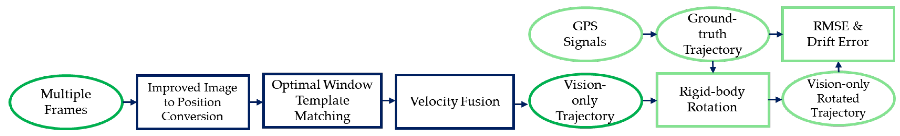
Figure 2.
Coordinate conversion functions: (a) horizontal direction, (b) vertical direction. The red circle indicates the center of the image.
Figure 2.
Coordinate conversion functions: (a) horizontal direction, (b) vertical direction. The red circle indicates the center of the image.
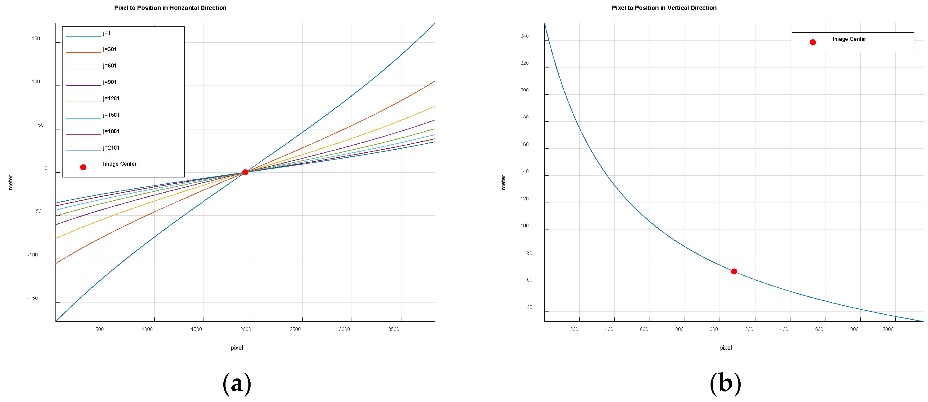
Figure 3.
(a) 10 linear segments, (b) 12 linear segments, (c) 15 linear segments.
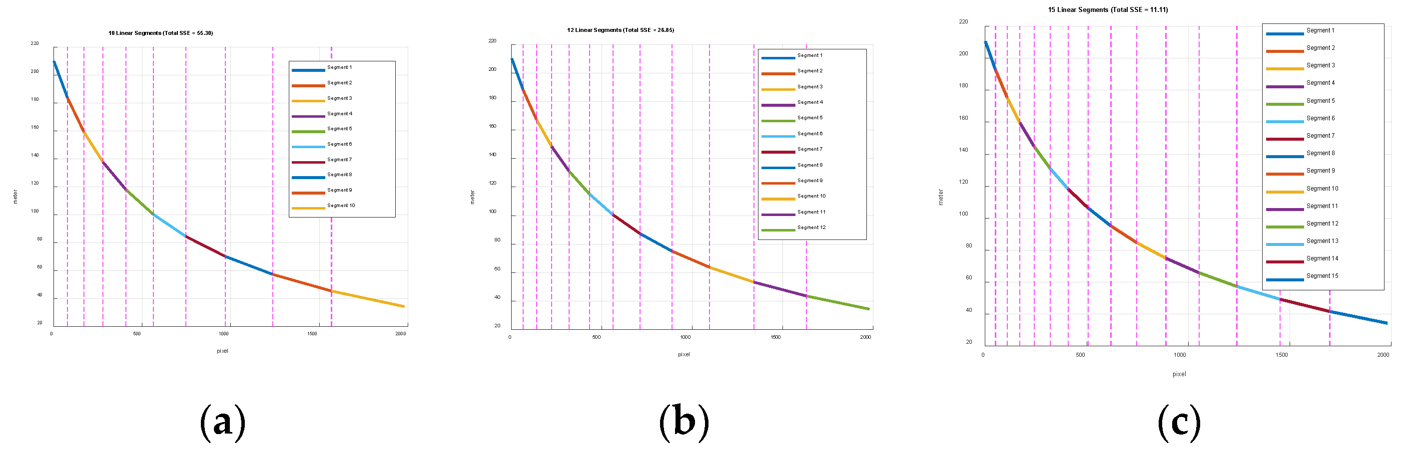
Figure 4.
Optimal windows corresponding to Figure 3, (a) 10 optimal windows, (b) 12 optimal windows, (c) 15 optimal windows. The centers of the windows are marked with a ‘+’.
Figure 4.
Optimal windows corresponding to Figure 3, (a) 10 optimal windows, (b) 12 optimal windows, (c) 15 optimal windows. The centers of the windows are marked with a ‘+’.
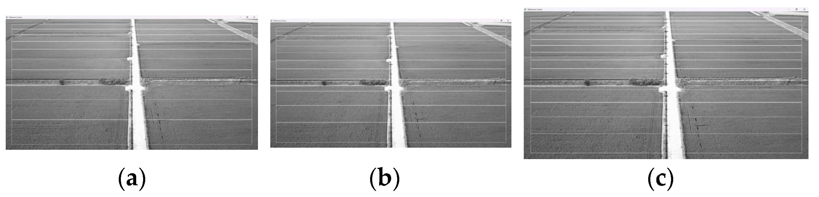
Figure 5.
Minimum detectable velocity, (a) horizontal direction, (b) vertical direction. The centers of the windows are marked with a ‘+’.
Figure 5.
Minimum detectable velocity, (a) horizontal direction, (b) vertical direction. The centers of the windows are marked with a ‘+’.
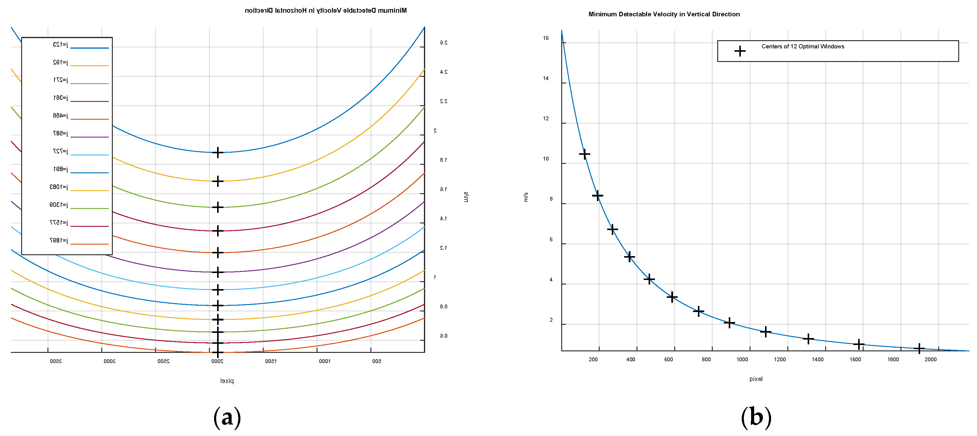
Figure 6.
Ground-truth trajectory obtained from GPS signals with starting (O), intermediate (A,B,C) and end (D) points, (a) Path 1, (b) Path 2, (c) Path 3, (d) Path 4, (e) Path 5, (f) Path 6.
Figure 6.
Ground-truth trajectory obtained from GPS signals with starting (O), intermediate (A,B,C) and end (D) points, (a) Path 1, (b) Path 2, (c) Path 3, (d) Path 4, (e) Path 5, (f) Path 6.
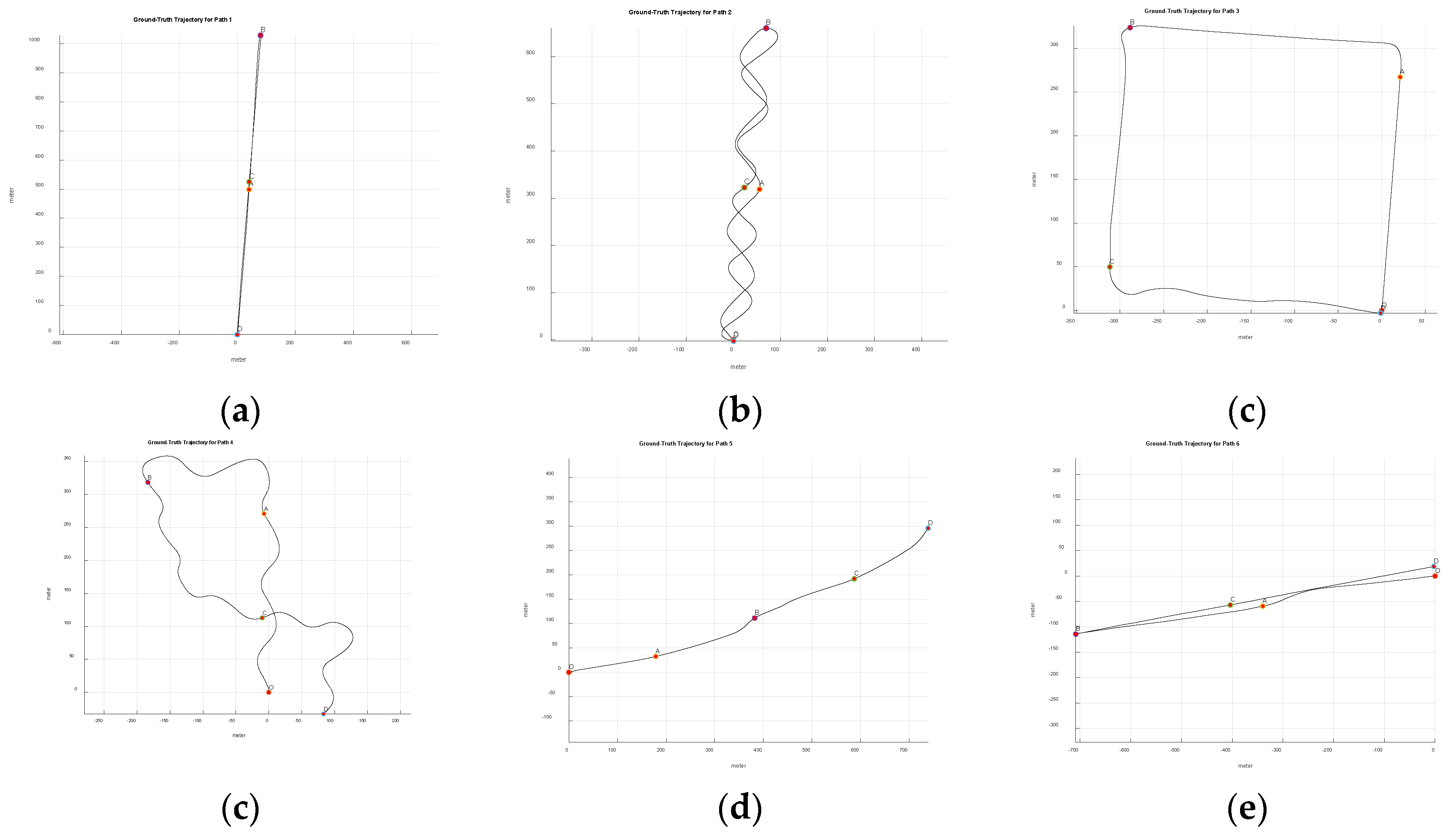
Figure 7.
Video frames at starting (O), intermediate (A, B, C), and end (D) point, (a) Path 1, (b) Path 2, (c) Path 3, (d) Path 4, (e) Path 5, (f) Path 6.
Figure 7.
Video frames at starting (O), intermediate (A, B, C), and end (D) point, (a) Path 1, (b) Path 2, (c) Path 3, (d) Path 4, (e) Path 5, (f) Path 6.
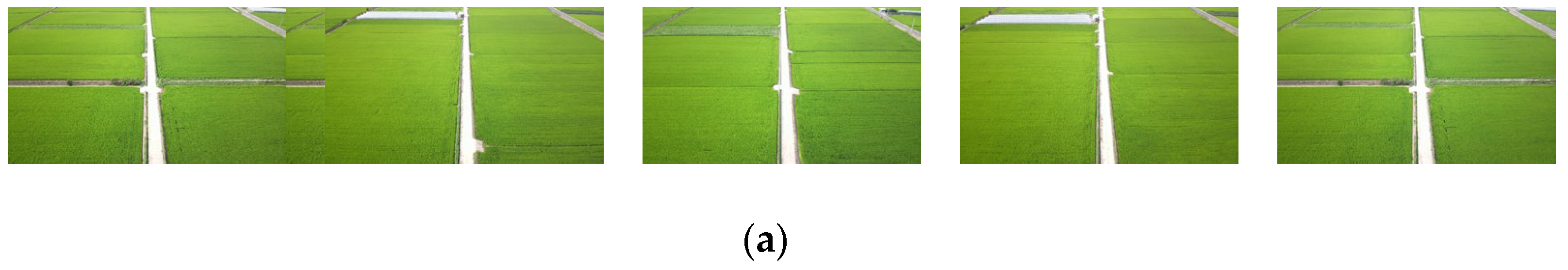
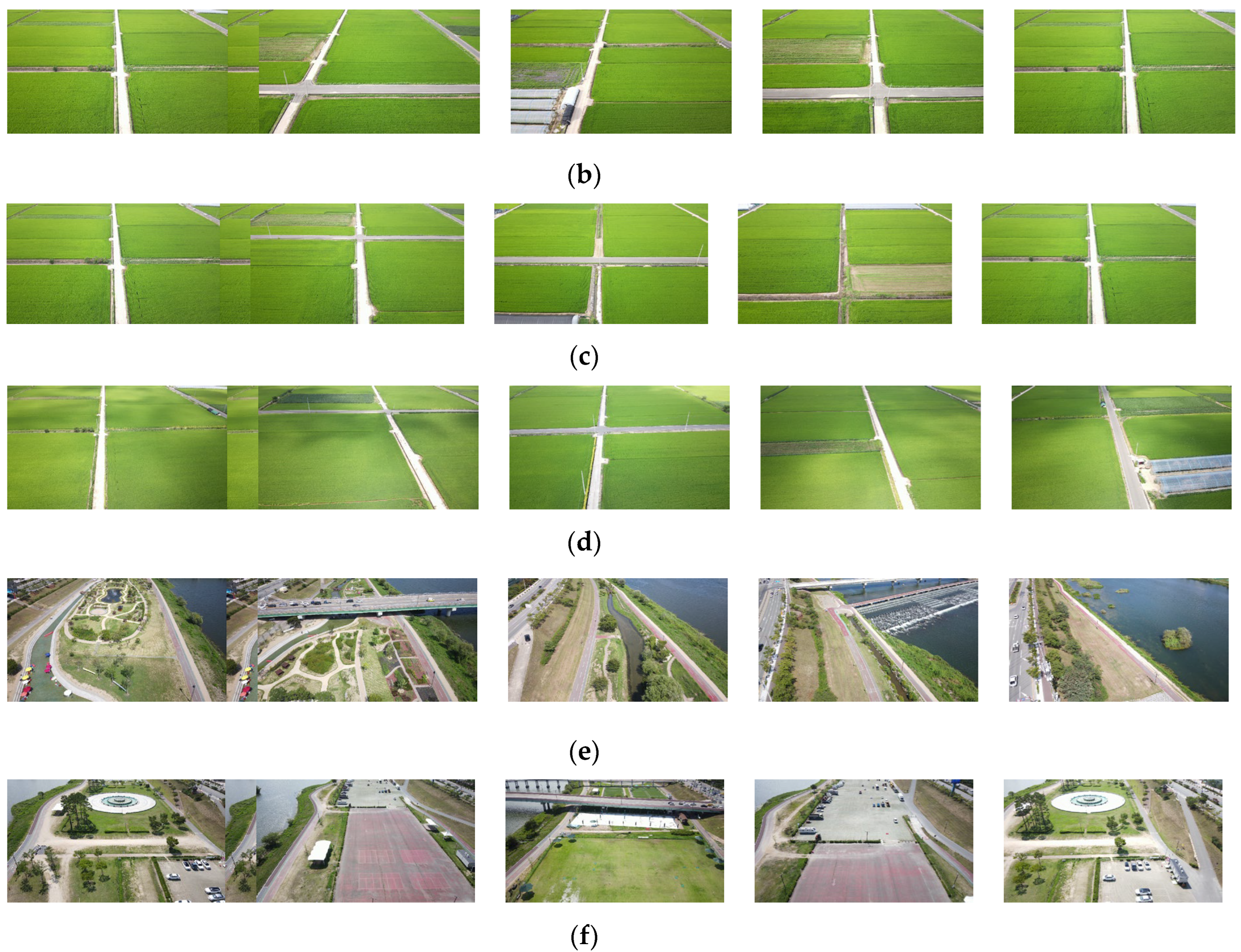
Figure 8.
Ground-truth trajectory and vision-only rigid-body rotated trajectory, (a) Path 1, (b) Path 2, (c) Path 3, (d) Path 4, (e) Path 5, (f) Path 6.
Figure 8.
Ground-truth trajectory and vision-only rigid-body rotated trajectory, (a) Path 1, (b) Path 2, (c) Path 3, (d) Path 4, (e) Path 5, (f) Path 6.
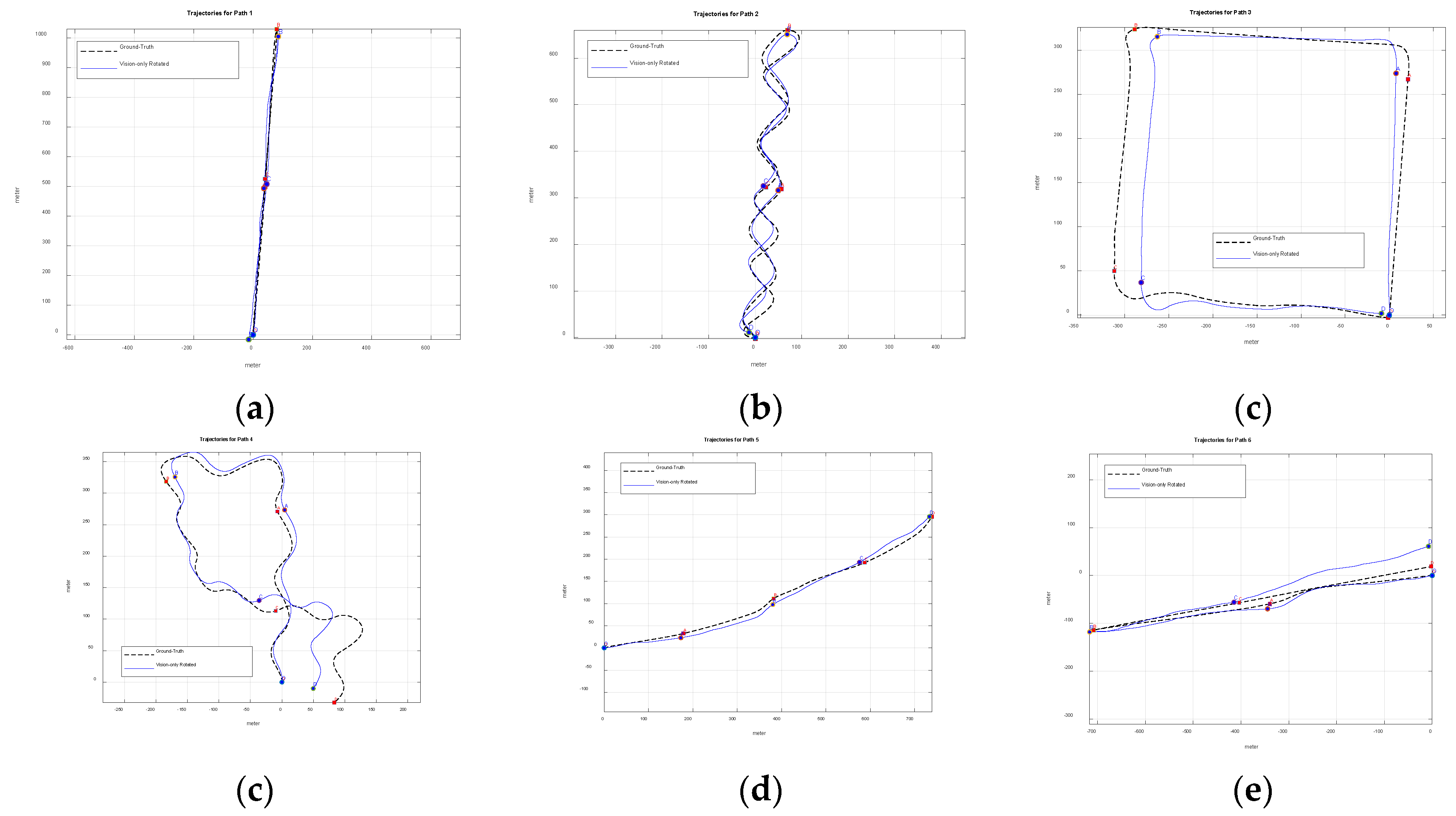
Figure 9.
Ground-truth velocity and vision-only rigid-body rotated velocity, (a) Path 1, (b) Path 2, (c) Path 3, (d) Path 4, (e) Path 5, (f) Path 6.
Figure 9.
Ground-truth velocity and vision-only rigid-body rotated velocity, (a) Path 1, (b) Path 2, (c) Path 3, (d) Path 4, (e) Path 5, (f) Path 6.
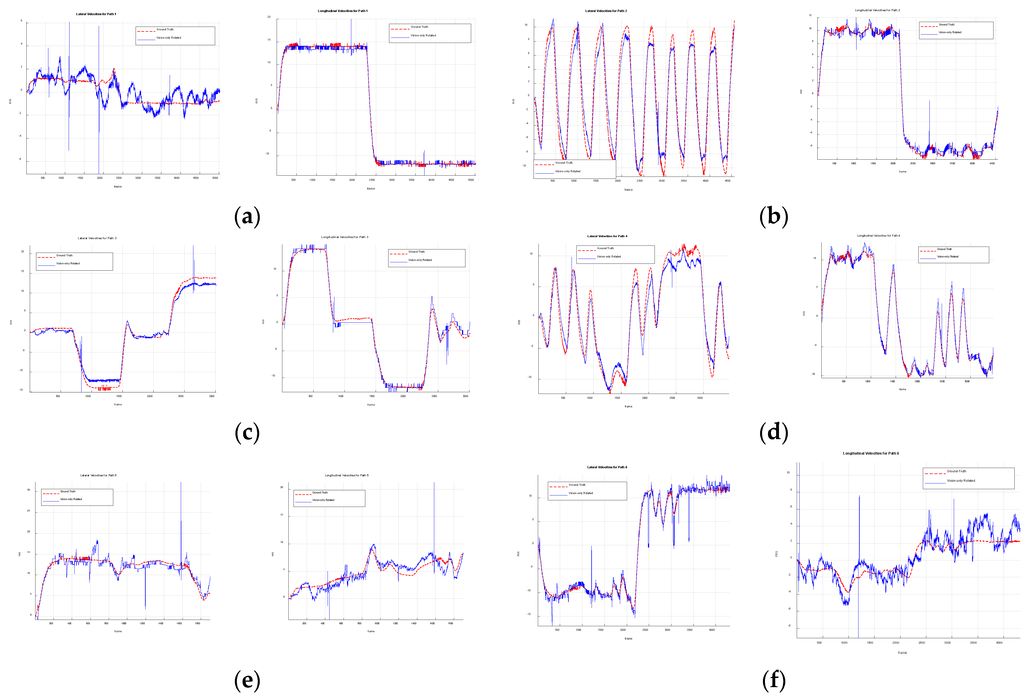
Figure 10.
Performance evaluation of zero-order hold scheme, (a) Path 1, (b) Path 2, (c) Path 3, (d) Path 4, (e) Path 5, (f) Path 6.
Figure 10.
Performance evaluation of zero-order hold scheme, (a) Path 1, (b) Path 2, (c) Path 3, (d) Path 4, (e) Path 5, (f) Path 6.
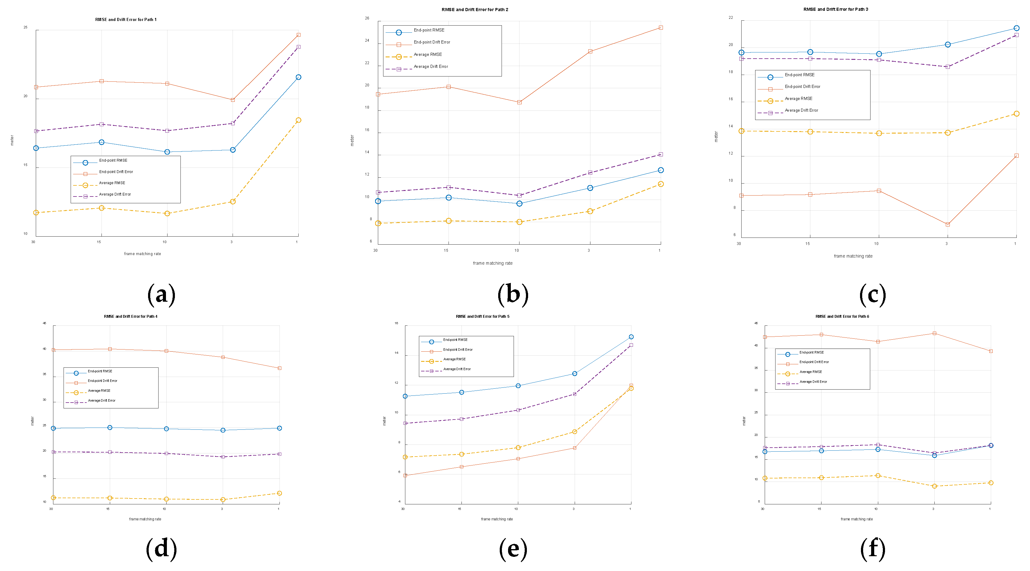

Table 1.
Frame number and path lengths of six paths.
|
Points |
Path 1 | Path 2 | Path 3 | Path 4 | Path 5 | Path 6 | |||||||
|---|---|---|---|---|---|---|---|---|---|---|---|---|---|
| Frame Number |
Path Length (m) |
Frame Number |
Path Length (m) |
Frame Number |
Path Length (m) |
Frame Number |
Path Length (m) |
Frame Number |
Path Length (m) |
Frame Number |
Path Length (m) |
||
| A | 1175 | 500.5 | 1063 | 398.7 | 678 | 268.35 | 866 | 302.19 | 476 | 182.05 | 1131 | 346.97 | |
| B | 2350 | 1033.1 | 2126 | 824.6 | 1482 | 611.45 | 1731 | 613.65 | 951 | 403.22 | 2261 | 720.68 | |
| C | 3686 | 1539.4 | 3367 | 1284.0 | 2242 | 891.84 | 2596 | 928.49 | 1426 | 624.12 | 3291 | 1031.44 | |
| D | 5021 | 2066.7 | 4560 | 1725.6 | 3013 | 1225.90 | 3462 | 1231.27 | 1901 | 810.99 | 4320 | 1440.1 | |
Table 2.
RMSE and drift error of six paths.
|
Points |
Path 1 | Path 2 | Path 3 | Path 4 | Path 5 | Path 6 | ||||||
|---|---|---|---|---|---|---|---|---|---|---|---|---|
| RMSE (m) |
Drift (m) |
RMSE (m) |
Drift (m) |
RMSE (m) |
Drift (m) |
RMSE (m) |
Drift (m) |
RMSE (m) |
Drift (m) |
RMSE (m) |
Drift (m) |
|
| A | 2.85 | 5.45 | 6.23 | 5.23 | 4.07 | 5.91 | 3.18 | 2.45 | 3.06 | 7.32 | 7.96 | 6.99 |
| B | 11.93 | 26.45 | 7.68 | 10.95 | 11.82 | 28.19 | 5.59 | 5.27 | 5.67 | 6.29 | 8.35 | 9.42 |
| C | 15.7 | 17.89 | 7.78 | 7 | 19.98 | 33.62 | 11.41 | 32.99 | 8.67 | 18.22 | 10.27 | 11.69 |
| D | 16.44 | 21.72 | 9.88 | 19.45 | 19.65 | 9.11 | 24.89 | 40.28 | 11.26 | 5.92 | 16.75 | 42.47 |
| Avg. | 11.73 | 17.88 | 7.89 | 10.66 | 13.88 | 19.21 | 11.27 | 20.25 | 7.17 | 9.44 | 10.83 | 17.64 |
Disclaimer/Publisher’s Note: The statements, opinions and data contained in all publications are solely those of the individual author(s) and contributor(s) and not of MDPI and/or the editor(s). MDPI and/or the editor(s) disclaim responsibility for any injury to people or property resulting from any ideas, methods, instructions or products referred to in the content. |
© 2025 by the authors. Licensee MDPI, Basel, Switzerland. This article is an open access article distributed under the terms and conditions of the Creative Commons Attribution (CC BY) license (http://creativecommons.org/licenses/by/4.0/).
Copyright: This open access article is published under a Creative Commons CC BY 4.0 license, which permit the free download, distribution, and reuse, provided that the author and preprint are cited in any reuse.


