
Submitted:
19 December 2025
Posted:
22 December 2025
You are already at the latest version
Abstract
Intensifying urbanisation in the Arctic, particularly in spatially constrained coastal and island cities, requires reliable information on long-term land use/land cover (LULC) change to assess environmental impacts and support urban planning. However, multi-decadal, high-resolution LULC datasets for Arctic cities remain limited. In this study, we quantify LULC change on Tromsøya (Tromsø, Norway) from 1984 to 2024 using multispectral satellite imagery based on Landsat and PlanetScope, complemented by LiDAR-derived canopy height models (CHM) and building footprints. We mapped LULC change trajectories and examined how these shifts relate to district-level population redistribution using gridded population data. The integration of a LiDAR-derived CHM was found to substantially improve the accuracy of Landsat-based LULC mapping and to represent the dominant source of classification gains, particularly for spectrally similar urban classes such as residential areas, roads, and other paved surfaces. Landsat augmented with CHM was shown to achieve practical equivalence to PlanetScope when the latter was modelled using spectral features only, supporting the feasibility of scalable and cost-effective long-term monitoring of urbanisation in Arctic cities. Based on the best-performing Landsat configuration, the proportions of artificial and green surfaces were estimated, indicating that approximately 20% of green areas were transformed into artificial classes. Spatially, population growth was concentrated in a small number of districts and broadly coincided with hotspots of green to artificial conversion The workflow provides a reproducible basis for long-term, district-scale LULC monitoring in small Arctic cities where data constraints limit consistent use of high-resolution image.
Keywords:
data fusion
; LiDAR
; canopy height model
; high-resolution imagery
; land use/land cover
; urbanisation
; global human population
; Tromsø
1. Introduction
Intensifying urbanisation is a globally prevalent phenomenon, which also occurs in the Arctic despite generally slower population growth [1,2,3]. Small and medium-sized Arctic cities experience infrastructure development, densification, and increasing connectivity with regional and global networks [4,5,6]. In some cases, notably that of Tromsø, Norway, these changes occur within highly constrained coastal and island environments, where development competes directly with limited green spaces and sensitive ecosystems [7,8,9,10,11]. As such, high-quality information on the long-term evolution of land use/land cover (LULC) is critical for analysing the environmental consequences of Arctic urban growth and for supporting evidence-based planning [12,13]. However, multi-decadal, high-resolution LULC datasets for Arctic cities remain extremely limited.
Existing global and circumpolar LULC products, such as CORINE, ESA WorldCover, and CALC-2020, can provide valuable baselines but have important limitations in Arctic urban settings [14,15,16,17,18,19,20,21,22]. Their spatial resolution (10-100 m), relatively coarse class definitions, and low temporal frequency restrict their ability to represent heterogeneous built-up patterns, green-urban mosaics, and narrow coastal margins [14,16,18,20,22].
While very high-resolution commercial imagery has been available for earlier years, its use for multi-decadal monitoring is often constrained by acquisition costs and incomplete temporal coverage for many locations. PlanetScope provides more systematic, high-frequency high-resolution observations, but only from 2017 onwards [23,24,25]. Consequently, no Arctic city currently has a continuous, multi-decadal LULC record at spatial scales appropriate for neighbourhood-level analysis. Landsat is the only publicly available satellite archive that spans four decades with consistent multispectral observations across the circumpolar region [26,27]. However, its 30 m spatial resolution poses substantial challenges in high-latitude urban environments, where buildings, roads, tree stands, and shoreline features frequently occupy areas smaller than a single pixel [28,29,30].
Recent advances in data fusion suggest that structural information derived from airborne LiDAR, and particularly canopy height models (CHM), can provide substantial benefits in discriminating spectrally similar urban classes and improving the delineation of built-up areas [25,28,29,30,31,32,33,34,35]. Although CHM-enhanced classification has been widely studied in forested and temperate urban environments [30,31,32,35,36,37], its performance in Arctic cities has not been systematically evaluated. Likewise, the potential of OpenStreetMap (OSM) building footprints to enhance LULC classification, particularly for small cities with mixed-density urban morphology, remains under-explored in high-latitude contexts [14,15,39].
An additional methodological gap concerns the operational equivalence of different sensor configurations for Arctic urban environments. It is currently unknown whether Landsat imagery, when supplemented with CHM and building context, can achieve classification performance comparable to high-resolution PlanetScope imagery [28,40,41,42,43]. This question has direct relevance for monitoring Arctic cities, where high-resolution imagery is often incomplete, costly, or unavailable for earlier decades [3,20,21,22,43]. Demonstrating that Landsat, integrated with auxiliary data, can approximate the performance of commercial sensors would offer a more accessible and scalable solution for long-term Arctic urban monitoring.
To address these gaps, this study develops and evaluates a multi-decadal LULC monitoring framework for Tromsøya (Tromsø, Norway) covering the period 1984-2024. Three feature configurations are tested for both Landsat and PlanetScope: (i) spectral reflectance only; (ii) spectral reflectance combined with LiDAR-derived canopy height; and (iii) spectral reflectance, canopy height, and rasterised OSM building footprints. This design allows us to (a) quantify the improvement in classification accuracy attributable to CHM and OSM features; (b) assess whether Landsat combined with CHM can deliver non-inferior performance relative to PlanetScope spectral-only data; and (c) evaluate cross-sensor consistency in class-area estimates using the overlap years 2017, 2020, and 2024.
Using the best-performing Landsat-based configuration, we then generate the first continuous 40-year LULC dataset for Tromsøya. This time series is used to quantify the dominant trajectories of change, including transitions between green and artificial surfaces, and modifications to the island coastline. Finally, we integrate LULC transitions with gridded population data (1985-2025) to examine how long-term patterns of land transformation relate to neighbourhood-level population redistribution - an essential but understudied dimension of Arctic urbanisation.
To our knowledge, this is the first study to (i) produce a multi-decadal, district-scale LULC dataset for an Arctic city; (ii) systematically evaluate the added value of CHM and OSM features for LULC mapping in Arctic urban environments; (iii) test practical equivalence between Landsat combined with CHM and PlanetScope spectral-only classifications; and (iv) link four decades of LULC change to population redistribution at district scale. The workflow provides a reproducible and cost-effective approach to long-term urban monitoring in high-latitude regions and offers new insights into the spatial structure and drivers of Arctic urban expansion.
2. Materials and Methods
2.1. Study Area
Tromsø is located along the Tromsø Fjord in Troms og Finnmark county, northern Norway (69.6° N, 18.9° E). Tromsøya is an island in Tromsø Municipality, Troms, situated between Kvaløya to the west and the mainland to the east. It is the largest urban area in Northern Norway and the fourth largest city north of the Arctic Circle [44]. Because of its geographic position and role in Arctic logistics and research, Tromsø is often described as a gateway to the High Arctic [2,3,44]. Tromsø is the 12th most populous municipality in Norway, with 78,745 residents, a population density of 31.2 inhabitants per km2, and approximately 10% growth over the previous ten years. The island covers an area of 21.7 km2 with 42,782 inhabitants in 2024 [45]. The urban area is situated within a narrow, ice-free fjord environment, bordered by steep mountain slopes. Land cover information indicates that the Tromsø municipality comprises a heterogeneous mosaic in which urban fabric is a substantial component alongside extensive forest cover [19,46]. The local climate is relatively mild for its latitude due to the influence of North Atlantic Ocean circulation [47]. Previous assessments further suggest that coastal areas in Northern Norway exhibit moderate to high vulnerability, with high to very high vulnerability reported for the island of Tromsø [48,49]. In this study, the analysis is restricted to the main island, as shown in Figure 1.
The primary reason for using Tromsøya as a case study is to test whether LiDAR-derived CHM can improve urban LULC mapping from multispectral imagery in high-latitude settings where medium-resolution pixels often mix buildings, roads, vegetation and shoreline. Norway has exceptional coverage of high-resolution airborne LiDAR, providing a strong basis for deriving CHM and better separating built and green surfaces in compact Arctic cities such as Tromsø [50]. Combined with Tromsøya’s constrained island geography and coastal mosaic, this makes it an ideal location for a transferable long-term monitoring workflow.
2.2. Data
2.2.1. Multispectral Imagery Features
As the multispectral information base for LULC classification, surface reflectance products from Landsat and PlanetScope were used to support multi decadal change analysis and high-resolution urban mapping for Tromsøya.
PlanetScope was selected as the high-resolution reference primarily because it provides near daily multispectral observations at around 3 m spatial resolution, and analysis ready, orthorectified surface reflectance scenes are delivered in four band and eight band configurations at Level 3B. This combination is well suited to quantitative LULC classification. Although very high-resolution commercial imagery has been available earlier and offers finer spatial detail, its use for systematic multispectral LULC mapping across multiple dates at city scale is often constrained by acquisition strategy and inconsistent temporal coverage, and such imagery frequently provides a more limited set of spectral bands for analysis [23,24].
Landsat Collection 2 surface reflectance products were acquired and processed via the Google Earth Engine platform. Imagery from the Landsat 8-9 Operational Land Imager and Landsat 4-5 Thematic Mapper sensors were utilised [26,27]. These sensors were selected because they provide consistent, high-quality multispectral data across a multi-decadal time, enabling robust long-term LULC change analysis.
The characteristics of the selected scenes and a summary of band correspondence are presented in the Supplementary Materials, Tables S1 to S3.
2.2.2. Structural Height and Building Footprint Features
To test whether structural information can improve the separation of spectrally similar urban classes, height and building footprint features were added as auxiliary predictors. Height information was derived from very high-resolution airborne LiDAR products obtained from the Norwegian national elevation data portal Høydedata [50]. Raster tiles covering the entire island of Tromsøya were downloaded, merged, and processed to derive a digital terrain model and a digital surface model, from which a canopy height model was calculated. Details of the LiDAR data used in this study are reported in the Supplementary Material, Table S4.
Building footprints were obtained from OpenStreetMap and used to derive building context layers for classification [14,15,39]. Footprints were filtered by building types where relevant and rasterised to the common analysis grid to produce binary predictor layers indicating the presence of residential and industrial buildings. Data were downloaded from https://www.openstreetmap.org/#map=12/69.6656/18.9976 (accessed on 30 September 2024).
2.3. Land Use/Land Cover Classification
Training and validation samples were prepared to support LULC classification in a heterogeneous urban environment. Mapping classes followed CLC Level 3 nomenclature and codes [19] and included water bodies, marsh land, grassland, coniferous forest, other trees, residential area, industrial area, roads and paved surfaces, and bare rocks. Class labels were assigned using the official CLC class characteristics, supported by the authors field observations in Tromsø in June 2025. Samples were labelled by visual interpretation of reference data, with recent years primarily supported by Google Maps imagery and earlier periods informed by a georeferenced topographic map (Topographic map 1990, M 711, 1534 3, 1:50,000) [61]. The full class rationale and local interpretation for Tromsøya are provided in the Supplementary Material, Table S5.
As additional quality control, median class spectral profiles and within class variability were examined for Landsat and PlanetScope. Details and plots are reported in the Supplementary Material, Figure S1.
Three feature configurations as models are tested for both Landsat and PlanetScope: (M1) spectral reflectance only; (M2) spectral reflectance combined with LiDAR-derived canopy height; and (M3) spectral reflectance, canopy height, and rasterised OSM building footprints. These models are applied to both Landsat imagery (2005-2024) and PlanetScope imagery (2017-2024), enabling assessment of classification performance across several years.
Let p denote a pixel on the common analysis grid with spatial resolution 3 m, x(p) denotes the feature vector (predictor vector) assigned to pixel p, S denote the set of surface reflectance bands used for a given sensor and year. SRs(p) is the surface reflectance value of bands s∈ S at pixel p. In this study S varies across sensors and PlanetScope product versions. For PlanetScope 2024 (8 bands), SPS = Coastal Blue, RGB, Green I, Yellow, Red Edge, and NIR. For PlanetScope 2020, 2017 (4 bands), SPS = RGB, and NIR and for Landsat 2024-1984, SL= RGB, NIR, SWIR1, and SWIR2.
The three models are defined as:
here CHM0(p) is the non-negative LiDAR-derived canopy height (in metres) aligned to the 3 m grid:
Bres, Bind rasterised binary building-context layers derived from OSM building footprints, aligned to the same 3 m grid. Both masks were produced by painting the filtered OSM footprint polygons into an empty image and applying unmask(0) so that background pixels are explicitly set to zero.
Model performance was evaluated using the confusion matrix (including producer’s and user’s accuracy per class), per-class, macro and weighted F1-scores, and balanced accuracy [56,57]. LULC classification was performed in Google Earth Engine, and the full processing scripts are available via the links provided in the Supplementary Materials.
To quantify categorical change between consecutive reference years, a vector-based post classification comparison workflow was applied. The resulting intersection polygons contained both from and to class attributes, enabling the computation of transition matrices and area statistics for each interval [58,59]. This workflow was used to quantify the transitions from green to artificial surfaces and the mapping of change hotspots.
2.4. Population Change Analysis
Residential population was derived from the Global Human Settlement Layer population grid (GHS POP, R2023A), which reports the number of residents per grid cell and provides estimates for 1985 to 2025 at five year intervals, with projections for 2030 [51,52]. To align with the LULC control years, population surfaces for 1985, 1990, 1995, 2000, 2005, 2015, 2020, and 2025 were extracted, clipped to the Tromsøya boundary, and harmonised to the study coordinate system. Tromsøya was subdivided into analysis districts based on postcode district boundaries, which were used as zoning units for district level aggregation. Each zone was assigned a conditional District ID (1-14) for visualisation and comparison. District population totals were computed by zonal summation and converted to population shares by normalising each district total by the Tromsøya total for the corresponding year. Changes in population share were then calculated to identify districts with relative gains or losses in residential population.
3. Results
3.1. Effect of Height and Building Footprint Features on Land use/Land Cover Classification Accuracy
3.1.1. Overall Performance Across Sensors and Years
Given these sensor specific differences within class variability, we next evaluate how adding height and building footprint information translates into measurable improvements in LULC classification performance across sensors and years. We compared three feature configurations (M1, M2, M3) to quantify the marginal contribution of CHM and OSM information and to test operational equivalence between sensors (Table 1).
According to Table 1, CHM is the principal driver of accuracy gains, with median ΔBA(M2-M1) of 6.48 for Landsat versus 3.32 for PlanetScope, indicating a stronger compensatory effect for the medium-resolution sensor. OSM provides a small but generally positive gain. For 2017-2024, M2 and M3 based on Landsat are non-inferior to Planet spectra-only within a margin [-0.81 to +1.31], indicating practical equivalence given cost and availability.
3.1.2. Class Level Gains
Beyond overall accuracy, per class mean F1 trajectories provide insight into where CHM and OSM reduce confusion among LULC categories, particularly within artificial surfaces and green surfaces classes (Figure 2).
According to Figure 2a, Landsat with M2 delivers the largest gains for residential area (25.8) and roads and paved surfaces (15.1). M3 yields only a small additional improvement for residential areas (4.7). For industrial areas, adding CHM has little positive effect, whereas adding OSM (3.0) sharpens the delineation of wide roofs. Natural classes such as coniferous forest and other trees also improve under M2, while M3 provides no meaningful additional benefit for these classes. Grassland benefits from CHM, whereas marsh land shows only a weak response to CHM. For PlanetScope (Figure 2b), despite the higher spatial resolution, CHM still has a strong effect for residential areas (13.5) and roads and paved surfaces (9.7). Industrial areas improve only slightly. Coniferous forest and other trees exhibit minor fluctuations, and the combined effect of M2 and M3 is close to zero. Marsh land and grassland show moderate gains with M2. Water bodies and bare rocks change minimally for both sensors because these classes are spectrally well separated.
3.1.3. Models’ Behaviour Through Class Specific Errors and Visual Validation
Class specific error analysis indicates that the main classification challenges are concentrated in a small set of class pairs with similar spectral characteristics or mixed urban morphology. The averaged class to class misclassification matrix, expressed as the percentage of the true class by sensor and model, is shown in Figure 3, while detailed producer and user accuracy values are reported in Supplementary Materials, Figure S2.
For Landsat, the baseline configuration shows the strongest confusion between residential area and roads and paved surfaces, with a substantial share of residential samples being mislabelled as paved classes, and additional confusion between residential and industrial areas (Figure 3a). After adding CHM, the dominant residential to roads confusion is markedly reduced, whereas residential to industrial confusion remains the principal residual challenge. Similarly, for roads and paved surfaces the primary error arises from mixing with residential areas, which is substantially reduced when CHM is included (Figure 3b), while the additional contribution of OSM for this class is minimal (Figure 3c). For industrial areas, height information alone does not consistently separate industrial and residential built forms. Instead, OSM provides the most evident incremental benefit by reducing industrial to residential mixing and increasing class purity (Figure 3c). The most persistent error pattern among natural classes is the mutual confusion between coniferous forest and other trees, observed for both sensors, together with leakage of grassland into tree classes. Additional confusion between grassland and marsh land is observed, consistent with closely related spectral signatures and a weaker response to structural predictors. For PlanetScope, the overall error structure is similar, CHM most strongly reduces residential to roads confusion (Figure 3e), but residential to industrial mixing partly persists even in M3 (Figure 3f).
According to Figure 4, using the 2024 scenes as examples, we can visually assess the classification accuracy and class delineation across all models and both sensors for Tromsø. The PlanetScope scene and the national orthophoto are used as high-resolution, up-to-date references, complemented by our field surveys conducted in June 2025. For water bodies, the main lakes such as Prestvannet, Langvannet, Lillevannet and Rundvannet are correctly mapped by all models and both sensors. As expected for a highly spectrally distinctive class. Notably, the Landsat-based models classify bare rocks along the western coastline more reliably (Figure 4d–f), plausibly due to the presence of the SWIR band. By contrast, PlanetScope models (Figure 4a–c) tend to confuse bare rocks with marsh land, industrial and residential area.
Despite spectral proximity to other artificial surface classes, M1 on both sensors (Figure 4a,d) separates large roads and paved surfaces units, reasonably well runways and aprons at the airport, shopping-centre car parks and other broad asphalted areas. Street networks within neighbourhoods, aprons and major car parks are visibly more coherent in M2 (Figure 4b,e), reducing mixing with industrial and residential areas. This effect is especially clear in the Landsat classifications (Figure 4d,e). M3 (Figure 4c,f) further regularises the boundaries between adjacent artificial classes.
For the industrial area, dominated by large warehouse roofs in the east, the shopping complex and parts of the UiT The Arctic University of Norway estate, M1 performs acceptably, with a clear advantage for PlanetScope (Figure 4a,d). M2 yields the most faithful interpretation on both sensors (Figure 4b,e). Some confusions with roads and paved surfaces persist along the aprons, and the boundaries are best damped in M3 (Figure 4c,f). The residential area shows the largest step-change from M1 to M2 and built-up blocks follow the real neighbourhood outlines, particularly for the Landsat-based maps, while PlanetScope M1 is already adequate. M3 mainly adds boundary regularisation, reducing stray green pixels within the built fabric. Substantial pixel mixing among artificial surface classes remains visible in all models.
The natural classes such as coniferous forest and other trees are spectrally well defined on both sensors and are generally represented consistently across models (Figure 4). Narrow urban shelterbelts remain challenging, especially for Landsat where M1 often underestimates them, and M2 only partly recovers these strips. Confusion between coniferous forest and other trees is substantial, peaking for Landsat M1. M3 reduces this uncertainty. Across both sensors, other trees and coniferous forest mixing also increases when moving between models. Our June 2025 field observations confirm the presence and distribution of coniferous forest patches across the island. For grassland (open lawns and verges), M2 and M3 improve overall accuracy, yet residual mixing with residential areas and other trees is common inside green neighbourhoods. The greatest confusion for grassland occurs with other trees on both sensors under M1. Marsh land is mapped well by all models, particularly in the northern concentrations. Misclassifications are modest with grassland and M2 and M3 reduce isolated false detections along shadowed forest edges by a small margin.
3.1.4. Cross Sensors Agreement in Class Areas
To characterise how differences in class areas arise, having established the most accurate configuration (M3), we next examine whether the resulting class area estimates are consistent between sensors in the overlap years. For transparency, the operational island extent in this analysis is defined by the classification mask, which includes inland water bodies, the intertidal and bare rock fringe, and land along the shoreline (Figure 5).
Figure 5a indicates that the most consistent agreement is observed for bare rocks and water bodies, while other trees and industrial areas also show generally stable differences between sensors. In contrast, the largest and most persistent discrepancies occur for residential areas, with Landsat systematically mapping a larger residential extent than PlanetScope under the common mask. Roads and paved surfaces also show substantial instability, and the direction of the sensor difference varies between years. Among natural classes, coniferous forest and grassland exhibit moderate, year dependent variability rather than a consistent bias, while marsh land is occasionally shows pronounced outlier differences.
The normalised transition matrix (Figure 5b) indicates that the strongest diagonal agreement is observed for other trees (84%), roads and paved surfaces (78%) and industrial area (67%), suggesting relatively stable class allocation between Landsat and PlanetScope for these categories. Moderate agreement is found for marsh land (56%), residential area (57%), coniferous forest (54%), grassland (51%) and water bodies (48%), implying more frequent cross-class reallocations. The most prominent systematic reallocations include coniferous forest to other trees (30%), grassland to other trees (19%), marsh land to grassland (26%), and residential area to roads and paved surfaces (18%). Bare rocks show the lowest diagonal agreement (24%), with substantial reassignment to industrial area (22%) and marsh land (20%), indicating limited cross-sensor consistency for this class within the coastal fringe.
3.3. Quantitative Analysis of Long-Term Land Use/Land Cover Changes in Tromsø from 1984 to 2024
The transition diagram (Figure 6) shows a clear long-term shift towards a larger share of artificial surfaces on Tromsøya.
In the early period (Figure 5a), when LULC was represented by four aggregated classes, artificial surfaces increased from 31% to 42%, while green surfaces (including grassland and trees) declined from 64% to 54%. Over the same interval, water bodies remain stable at about 3-4%, indicating that the main changes are driven by urban expansion rather than changes in inland water extent. From 2005 onwards, the analysis is reported using the expanded nine class scheme, which becomes feasible once height information is incorporated, improving separation of structurally similar urban and vegetation types. This reveals how the urban fraction is partitioned across specific built-up categories (Figure 6b). Roads and paved surfaces form the single largest component throughout 2005-2024 (about 32-38%). The built-up fabric becomes more differentiated over time, in particular, industrial area increases from 4% (2005) to 8% (2024), while residential area remains of comparable magnitude but shows a gradual decline from 11% to 9%. Green surface area remains substantial and relatively stable in proportional terms, with other trees around 17-19% and grassland around 14-17%, while coniferous forest constitutes a smaller but persistent share (about 4-5%). Marsh land decreases from 8% in 2005 to 4% in 2024, suggesting either contraction or systematic reallocation of marginal wetland areas to adjacent vegetated classes. The direct 1984-2024 comparison (Figure 6c) confirms sustained urbanisation, driven mainly by the expansion and persistence of transport related artificial surfaces, alongside increasing industrial land use and declining shares of green surfaces and wetland covers.
Using a pixel-based change detection analysis, we can clearly identify spatial hotspots of the largest changes in LULC class areas (Figure 7). Changes are evident across the whole island, but they are most pronounced in northern Tromsøya, particularly around Hamna. Shoreline change is also apparent, in the north-eastern part of the island, the coastline has shifted mainly due to the conversion of parts of the water area into paved surfaces (Figure 7a).
The maps in Figure 7 reveal a pronounced expansion and consolidation of artificial surfaces between 1984 and 2024, with the island-wide balance shifting from 64% green and 31% artificial surfaces in 1984 (Figure 7c) to 44% green and 55% artificial surfaces in 2024 (Figure 7b). Overall, 20% of the green surface area transitions to artificial surface classes, and these conversions are spatially clustered with the largest hotspots associated with the main built-up and transport-related surfaces, consistent with long term urbanisation across Tromsøya (Figure 7a).
3.4. Population Patterns in Relation to Land Cover Change
This subsection examines how residential population redistribution across Tromsøya relates to long term changes in the balance between green and artificial surfaces. Population redistribution is spatially uneven (Figure 8).
The largest relative gains in population share are concentrated in District 8 (133%) and District 11 (121%), with a secondary hotspot in District 12 (60%). The embedded LULC bars indicate that districts with the strongest population-share gains generally coincide with a larger shift towards artificial surfaces between 1984 and 2024. Spatially, these population-share gain districts broadly align with the main green to artificial conversion hotspots mapped in Figure 7a, particularly in areas characterised by recent development footprints.
4. Discussion
4.1. Classification Uncertainties and Their Influence on the Results
Some uncertainty in the mapped urban LULC patterns is likely to arise from differences in the native spatial resolution of the input datasets and the need to harmonise all predictors to a common 3 m analysis grid. Resampling Landsat to the PlanetScope grid improves geometric alignment for comparison but does not add spatial detail, so boundaries, narrow linear features, and fine scale urban mosaics may remain affected by mixed pixel effects in medium resolution imagery [32,33,34,35,36,37,38]. Additional uncertainty may be introduced by the aggregation of LiDAR derived canopy height information from sub metre products to 3 m, which can smooth small objects and dampen local height extremes in heterogeneous neighbourhoods [40]. Residual confusion among built classes may also reflect heterogeneous materials, shadowing, and limitations in vector to raster alignment for building footprint layers, rather than height information alone [41,42,43]. Finally, it is important to consider temporal misalignment of ancillary layers with specific mapping years. For example, LiDAR is available for discrete years, while OSM reflects the state of the built environment at the time of contribution and updating. This may locally affect class estimates in rapidly changing areas, but it does not change the overall interpretation of the dominant trends supported by accuracy metrics, error structures and map-based evidence.
Some these issues were addressed by using spatial block cross validation, testing multiple feature configurations, and interpreting change patterns in the context of class specific performance diagnostics and map-based evidence. Future work could further reduce uncertainty by incorporating temporally matched structural data where available, applying additional shadow and illumination normalisation, improving footprint quality control, and expanding reference data with independent ground truth or higher frequency validation for rapidly changing urban areas.
4.2. Comparison with Other Similar Studies
The regularities obtained in this study are consistent with previous work on the fusion of optical data and LiDAR, where height features (CHM) systematically improve thematic classification quality, especially for structurally complex urbanised classes. In particular, in studies [13,28,29,30,31,32,33] the authors note that spectral features are insufficient for classifying trees in a city because of the high spectral similarity of species, whereas integrating CHM substantially increases accuracy, and CHM itself acts as one of the most influential predictors. Thus, for the task of mapping shrub communities [35,41] and vegetation area [29,53], the authors applied models based on Landsat predictors, SPOT and PlanetScope that were trained on CHM, and which effectively distinguish shrubs, young forest and other vegetation from other classes. In study [13,38], the authors used the integration of vegetation indices and CHM and improved the separation of built-up and vegetated types, refining change analysis in the context of urbanisation and greening. This directly supports the interpretation of our results, since Landsat in combination with CHM compensated for the mixed-pixel effect (Table 1) and increases separability of structurally different but spectrally similar classes. In particular, the grassland class was well separated from the coniferous forest and other trees classes (Fig. 3). Unlike many previous studies that evaluate fusion mainly within a single year or a single sensor [28,29,30], in our work the CHM effect is traced across several years and linked to the practical issue of the reproducibility of long-term monitoring. It is shown that Landsat configurations with CHM in the overlap years provide practically equivalent quality to the spectral PlanetScope model, which strengthens the argument for reliable mapping under conditions of limited availability of high-resolution imagery. In addition, the analysis of cross-sensor area consistency and the normalised transition matrix allow interpretation not only of metric gains, but also of the nature of systematic reallocations of area between classes, which is less often considered in studies focused only on accuracy metrics.
It is also important to note that a wide range of ready-to-use LULC products is currently available at global and regional scales, including datasets that cover the Arctic. For instance, the OSM Landuse/Landcover dataset [14,15] provides an OSM-informed classification framework broadly comparable to Level 2 of the CORINE Land Cover legend and can be readily integrated into standard GIS workflows. It is derived from Sentinel-2 imagery using a deep-learning model trained on OSM land-use and land-cover features. It is a classification of Sentinel-2 imagery using a deep learning model trained on OSM landuse and landcover features [15]. The ESA WorldCover product [16,17] offers global land-cover maps for 2020 and 2021 at 10 m spatial resolution, developed and validated in near-real time using Sentinel-1 and Sentinel-2 observations. The Sentinel-2 10-m Land Use/Land Cover product [18], generated using artificial intelligence and large-scale human-labelled training data, provides predictions for nine classes and includes an annual time series for 2017-2021 available via the Living Atlas. In Europe, the CLC inventory provides a pan-European land-cover and land-use dataset with 44 thematic classes and is updated at six-year intervals, with the most recent update reported for 2018 [19]. For the circumpolar domain, the Arctic LULC product for circa 2020 (CALC-2020) integrates Sentinel-1 polarisation, Sentinel-2 surface reflectance, and ArcticDEM topographic variables within a machine-learning framework to map dominant biophysical components at 10 m resolution using ten generic classes [20,21]. In addition, recent work has demonstrated Landsat-based machine-learning mapping of urban change in Tromsø, including impervious surface dynamics over 1993-2023 [22].
These products provide valuable broad-scale context, but within the scope of this study they are best viewed as complementary rather than as a substitute for local mapping. They are typically optimised for large-area applications and differ in nomenclature, analysis masks and temporal focus, which complicates direct comparisons in a small, highly heterogeneous urban setting. For Tromsøya, narrow transport elements, fragmented built fabric and mixed urban materials (Figure 2, Figure 3 and Figure 4) can lead to generalisation or heightened sensitivity to shadowing and mixed pixels in products with coarser thematic or spatial representation. Moreover, most ready-made maps focus on single contemporary years or relatively short time series [14,15,16,17], whereas reconstructing 1984-2024 dynamics requires a consistent retrospective framework. In this sense, combining the long Landsat archive with height information enables interpretation of long-term transitions between green and artificial surfaces and supports finer differentiation of urban components in recent years (Figure 6 and Figure 7).
A relevant local comparison is the study [22], which mapped urban change in the Tromsø region using a binary impervious and non-impervious Landsat-based approach for 1993-2023. Despite differences in approach and spatial extent, both analyses indicate sustained growth of artificial surfaces and a stronger change signal in the later period, consistent with our trajectories (Figure 6) and spatial patterns of conversion (Figure 7). However, our multi-class LULC nomenclature enables urbanisation to be decomposed into roads and paved surfaces, residential and industrial area, allowing a more detailed interpretation of the processes underlying change (Figure 7). In addition, the district-level population analysis shows that population-share gains are concentrated in a small number of districts (Figure 8) and align with hotspots of green to artificial transitions (Figure 7a), extending ISA-based interpretations by linking LULC change to demographic redistribution at an urban scale.
4.3. Population Redistribution and the Shift from Green to Artificial Surfaces
Comparing the pixel-based hotspots of LULC change (Figure 7a) with district-level demographic redistribution (Figure 8) reveals a broadly consistent spatial signal of urbanisation. Areas with the most intensive transitions from green to artificial surfaces in Figure 7a are concentrated in the north of the island and along key development and transport corridors, and these same districts in Figure 8 tend to show the largest gains in population share, suggesting a link between expansion or intensification of the built environment and the concentration of residents in a small number of districts. At the same time, some pronounced LULC transitions may be only weakly reflected in demographic change, while population gains can also arise through densification within already urbanised areas without large net losses of green space. Together, these aligned and partly decoupled patterns indicate that urbanisation on Tromsøya is shaped by two parallel processes: (i) spatial expansion of artificial surfaces at the expense of green areas in distinct hotspots, and (ii) demographic redistribution between districts that does not necessarily require proportional growth in built-up area but may reflect changes in housing density and LULC function.
5. Conclusions
This study developed and evaluated a transferable remote sensing workflow for multi decadal, district scale urban LULC monitoring in small Arctic cities. LiDAR derived CHM was found to provide the dominant and most consistent accuracy improvement for urban LULC classification, particularly when medium resolution multispectral imagery is used. By incorporating CHM, Landsat based mapping was substantially strengthened for spectrally similar and heterogeneous built classes, and Landsat with CHM achieved practical equivalence to spectral only PlanetScope during the overlap years, according to the evaluation metrics reported. This indicates that robust long-term monitoring can be achieved with reduced reliance on continuous high resolution commercial imagery, where structural predictors are available for calibration and performance enhancement. OpenStreetMap building footprints provided a smaller but generally positive contribution, mainly by refining within urban boundaries and reducing confusion between built classes.
The strongest class specific gains from CHM were observed for the most heterogeneous artificial classes, particularly residential areas and roads and paved surfaces, where mixed pixels, material diversity, and shadow effects limit purely spectral separation. Cross sensor agreement in mapped class areas was clearly class dependent, and several classes showed systematic reallocations between related categories, indicating that changes in sensor inputs can affect not only headline accuracy metrics but also the inferred class area balance. This consideration is important when interpreting long term trajectories and comparing results across sensors.
Applied to Tromsøya, the resulting time series indicates that long term, neighbourhood scale urban change in Arctic cities can be quantified more consistently when multispectral archives are strengthened with structural and contextual predictors. The integration of Landsat with LiDAR derived canopy height, enables more reliable delineation of green to artificial conversions, infrastructure related expansion, and localised shoreline modification than spectral information alone, particularly in heterogeneous coastal settings. In addition, the workflow supports reproducible hotspot-based monitoring, providing an operational evidence base for identifying where land transformation is concentrated and for prioritising planning responses such as protecting and reconnecting green corridors, targeting compensatory greening, and managing densification pressures using comparable indicators across years rather than single year map interpretation.
Supplementary Materials
The following supporting information can be downloaded at the website of this paper posted on Preprints.org. The following supporting information will be available for download from the University of Cambridge Apollo repository, and a link will provide above. At the time of submission, these materials have not yet been uploaded and will be deposited upon acceptance of the manuscript for publication: Table S1, information on the PlanetScope scenes used in this study; Table S2, information on the Landsat scenes used in this study; Table S3, correspondence of PlanetScope and Landsat spectral bands used in the study; Table S4, LiDAR datasets used in the study; Table S5, full class definitions (CLC Level 3), local interpretation for Tromsøya, and sample justification; Figure S1, multi sensor spectral signatures of LULC training and validation samples; Figure S2, distributions of producer and user accuracy averaged across 2005 to 2024 by sensor and model (M1, M2, M3); and links for GEE code.
Author Contributions
Conceptualization, L.H.B. and G.R.; methodology, L.H.B. and G.R; software, L.H.B.; validation, L.H.B., G.R. and S.W.; formal analysis, L.H.B. and G.R.; resources, L.H.B., G.R., S.W. and V.B.; data curation, L.H.B., G.R. and S.W.; writing—original draft preparation, L.H.B., G.R. and S.W; writing—review and editing, L.H.B., G.R., S.W. and V.B.; visualization, L.H.B. and G.R.; supervision, L.H.B. and G.R.; funding acquisition, L.H.B., G.R. and S.W. All authors have read and agreed to the published version of the manuscript.
Funding
This research was funded by the British Academy, Cara, Leverhulme Researchers at Risk Research Support Grants 2024, LTRSF24\100036 under the project «Hotter Arctic cities: mitigating Urban Heat Islands with spatial data, community insights, and sustainable solutions».
Institutional Review Board Statement
Not applicable.
Informed Consent Statement
Not applicable.
Data Availability Statement
Data is contained within the article.
Acknowledgments
Lillia Hebryn-Baidy expresses her gratitude to the British Academy and the Council for At-Risk Academics for providing support to this research study through the Researchers at Risk Research Support Grants. Sincere gratitude goes to the Scott Polar Research Institute, University of Cambridge for their support throughout the research process.
Conflicts of Interest
The authors declare no conflicts of interest.
References
- Dybbroe, S.; Dahl, J.; Müller-Wille, L. Dynamics of Arctic Urbanization. Acta Borealia 2010, 27, 120–124. [Google Scholar] [CrossRef]
- Laruelle, M. The three waves of Arctic urbanisation. Drivers, evolutions, prospects. Polar Record. 2019, 55, 1–12. [Google Scholar] [CrossRef]
- Miles, V.; Esau, I.; Miles, M.W. The urban climate of the largest cities of the European Arctic. Urban Climate 2023, 48. [Google Scholar] [CrossRef]
- Meredith, M.; Sommerkorn, M.; Cassotta, S.; Derksen, C.; Ekaykin, A.; Hollowed, A.; Kofinas, G. A. Mackintosh, J. Melbourne-Thomas, M.M.C. Muelbert, G. Ottersen, H. Pritchard, and E.A.G. Schuur, 2019: Polar Regions. In IPCC Special Report on the Ocean and Cryosphere in a Changing Climate [H.-O. Pörtner; Roberts, D.C., Masson-Delmotte, V., Zhai, P., Tignor, M., Poloczanska, E., Mintenbeck, K., Alegría, A., Nicolai, M., Okem, A., Petzold, J., Rama, B., Weyer, N.M., Eds.; Cambridge University Press: Cambridge, UK and New York, NY, USA; pp. 203–320. [CrossRef]
- Heleniak, T. The future of the Arctic populations. Polar Geography 2020, 44, 136–152. [Google Scholar] [CrossRef]
- Wehrmann, D.; Luszczuk, M.; Radzik-Maruszak, K.; Götze, J.; Riedel, A. Sustainable Urban Development in the European Arctic; Routledge, 2025. [Google Scholar] [CrossRef]
- Soroudi, A.; Rizzo, A.; Ma, J. Urban Sustainability in Arctic Cities: Challenges and Opportunities of Implementing the Sustainable Development Goals. Urban Planning 2024, 9, 8349. [Google Scholar] [CrossRef]
- Soroudi, A.; Aboagye, P.D.; Ma, J.; et al. Downscaling the sustainable development goals for the Arctic cities. npj Urban Sustain 2025, 5, 16. [Google Scholar] [CrossRef]
- López-Blanco, E.; Topp-Jørgensen, E.; Christensen, T.R.; et al. Towards an increasingly biased view on Arctic change. Nat. Clim. Chang. 2024, 14, 152–155. [Google Scholar] [CrossRef]
- Hebryn-Baidy, L.; Rees, G. Evaluating Urban Heat Island Dynamics and Land Use/Land Cover Changes in Tromsø, Norway. International Conference of Young Professionals "GeoTerrace 2024", Oct 2024; Vol. 2024, pp. 1–5. [Google Scholar] [CrossRef]
- Rees, G.; Hebryn-Baidy, L.; Good, C. Estimating the Potential for Rooftop Generation of Solar Energy in an Urban Context Using High-Resolution Open Access Geospatial Data: A Case Study of the City of Tromsø, Norway. ISPRS Int. J. Geo-Inf. 2025, 14, 123. [Google Scholar] [CrossRef]
- Yu, D.; Fang, C. Urban Remote Sensing with Spatial Big Data: A Review and Renewed Perspective of Urban Studies in Recent Decades. Remote Sens. 2023, 15, 1307. [Google Scholar] [CrossRef]
- Morsy, S.; Shaker, A.; El-Rabbany, A. Multispectral LiDAR Data for Land Cover Classification of Urban Areas. Sensors 2017, 17, 958. [Google Scholar] [CrossRef] [PubMed]
- Schultz, M.; Voss, J.; Auer, M.; Carter, S.; Zipf, A. Open land cover from OpenStreetMap and remote sensing. International Journal of Applied Earth Observation and Geoinformation 2017, 63, 206–213. [Google Scholar] [CrossRef]
- Schultz, Michael; Li, Hao; Wu, Zhaoyhan; Wiell, Daniel; Auer, Michael; Zipf, Alexander. OpenStreetMap Land Use for Europe & quot; Research Data" heiDATA, 2024. [Google Scholar] [CrossRef]
- Zanaga, D.; Van De Kerchove, R.; De Keersmaecker, W.; Souverijns, N.; Brockmann, C.; Quast, R.; Wevers, J.; Grosu, A.; Paccini, A.; Vergnaud, S.; Cartus, O.; Santoro, M.; Fritz, S.; Georgieva, I.; Lesiv, M.; Carter, S.; Herold, M.; Li, Linlin; Tsendbazar, N.E.; Ramoino, F.; Arino, O. ESA WorldCover 2021, 10 m 2020 v100. [CrossRef]
- Zanaga, D.; Van De Kerchove, R.; Daems, D.; De Keersmaecker, W.; Brockmann, C.; Kirches, G.; Wevers, J.; Cartus, O.; Santoro, M.; Fritz, S.; Lesiv, M.; Herold, M.; Tsendbazar, N.E.; Xu, P.; Ramoino, F.; Arino, O. ESA WorldCover 10 m 2021 v200. 2022. [Google Scholar] [CrossRef]
- Karra, Kontgis; et al. Global land use/land cover with Sentinel-2 and deep learning. IGARSS 2021-2021 IEEE International Geoscience and Remote Sensing Symposium; IEEE, 2021; Available online: https://livingatlas.arcgis.com/landcover/.
- European Union's Copernicus Land Monitoring Service information. Available online: https://land.copernicus.eu/en/products/corine-land-cover.
- Liu, C.; Xu, X.; Feng, X.; Cheng, X.; Liu, C.; Huang, H. : CALC-2020: a new baseline land cover map at 10 m resolution for the circumpolar Arctic. Earth Syst. Sci. Data 2023, 15, 133–153. [Google Scholar] [CrossRef]
- Xu, Xiaoqing; Liu, Chong; Liu, Caixia; et al. Circumpolar Arctic Land Cover for circa 2020 (CALC-2020)[DS/OL]. V1. In Science Data Bank; 2022[2025-11-24. [Google Scholar] [CrossRef]
- Dermosinoglou, K.; Detsikas, S.E.; Petropoulos, G.P.; Fratsea, L.M.; Papadopoulos, A.G. Chapter 17 - Multi-temporal monitoring of impervious surface areas (ISA) changes in an Arctic setting, using ML, remote sensing data, and GEE. In Earth Observation, Google Earth Engine and Artificial Intelligence for Earth Observation; Elsevier, 2025; pp. 321–348. [Google Scholar] [CrossRef]
- Planet Documentation. Available online: https://docs.planet.com/data/imagery/arps/techspec/.
- Acharki, S. PlanetScope contributions compared to Sentinel-2, and Landsat-8 for LULC mapping. Remote Sensing Applications: Society and Environment 2022, 27, 100774. [Google Scholar] [CrossRef]
- Szostak, M.; Likus-Cieślik, J.; Pietrzykowski, M. PlanetScope Imageries and LiDAR Point Clouds Processing for Automation Land Cover Mapping and Vegetation Assessment of a Reclaimed Sulfur Mine. Remote Sens. 2021, 13, 2717. [Google Scholar] [CrossRef]
- Earth Resources Observation and Science (EROS) Center. Landsat 8-9 Operational Land Imager / Thermal Infrared Sensor Level-2, Collection 2 [dataset]. In U.S. Geological Survey; 2020. [Google Scholar] [CrossRef]
- Earth Resources Observation and Science (EROS) Center. Landsat 4-5 Thematic Mapper Level-2, Collection 2 [dataset]. In U.S. Geological Survey; 2020. [Google Scholar] [CrossRef]
- Dong, P.; Ramesh, S.; Nepali, A. Evaluation of small-area population estimation using LiDAR, Landsat TM and parcel data. International Journal of Remote Sensing 2010, 31, 5571–5586. [Google Scholar] [CrossRef]
- Vizzari, M.; Antonielli, F.; Bonciarelli, L.; Grohmann, D.; Menconi, M. Urban greenery mapping using object-based classification and multi-sensor data fusion in Google Earth Engine. Urban Forestry & Urban Greening 2025, 105, 128697. [Google Scholar] [CrossRef]
- Shimizu, K.; Ota, T.; Mizoue, N.; Saito, H. Comparison of Multi-Temporal PlanetScope Data with Landsat 8 and Sentinel-2 Data for Estimating Airborne LiDAR Derived Canopy Height in Temperate Forests. Remote Sens. 2020, 12, 1876. [Google Scholar] [CrossRef]
- Chi, D.; Yan, J.; Yu, K.; Morsdorf, F.; Somers, B. Planting contexts affect urban tree species classification using airborne hyperspectral and LiDAR imagery. Landscape and Urban Planning 2025, 257, 105316. [Google Scholar] [CrossRef]
- Yao, Y.; Wang, X.; Qin, H.; Wang, W.; Zhou, W. Mapping Urban Tree Species by Integrating Canopy Height Model with Multi-Temporal Sentinel-2 Data. Remote Sens. 2025, 17, 790. [Google Scholar] [CrossRef]
- Kumaraperumal, R.; Raj, M.N.; Pazhanivelan, S.; et al. Data mining techniques for LULC analysis using sparse labels and multisource data integration for the hilly terrain of Nilgiris district, Tamil Nadu, India. Earth Sci Inform 2025, 18, 13. [Google Scholar] [CrossRef]
- Tolentino, F.; Galo, M. Selecting features for LULC simultaneous classification of ambiguous classes by artificial neural network. Remote Sensing Applications: Society and Environment 2021, 24, 100616. [Google Scholar] [CrossRef]
- Mahoney, M. J.; Johnson, L. K.; Guinan, A. Z.; Beier, C. M. Classification and mapping of low-statured shrubland cover types in post-agricultural landscapes of the US Northeast. International Journal of Remote Sensing 2022, 43, 7117–7138. [Google Scholar] [CrossRef]
- Lin, C.; Doyog, N.D. Challenges of Retrieving LULC Information in Rural-Forest Mosaic Landscapes Using Random Forest Technique. Forests 2023, 14, 816. [Google Scholar] [CrossRef]
- Nordkvist, K.; Granholm, A. H.; Holmgren, J.; Olsson, H.; Nilsson, M. Combining optical satellite data and airborne laser scanner data for vegetation classification. Remote Sensing Letters 2011, 3, 393–401. [Google Scholar] [CrossRef]
- Lin, MH.; Lin, YT.; Tsai, ML.; et al. Mapping land-use and land-cover changes through the integration of satellite and airborne remote sensing data. Environ Monit Assess 2024, 196, 246. [Google Scholar] [CrossRef] [PubMed]
- Biljecki, F.; Chow, Y.S.; Lee, K. Quality of crowdsourced geospatial building information: A global assessment of OpenStreetMap attributes. Build. Environ. 2023, 237, 110295. [Google Scholar] [CrossRef]
- Jin, Huiran; Mountrakis, Giorgos. Fusion of optical, radar and waveform LiDAR observations for land cover classification. ISPRS Journal of Photogrammetry and Remote Sensing 2022, 187, 171–190. [Google Scholar] [CrossRef]
- Ziegelmaier Neto, B.H.; Schimalski, M.B.; Liesenberg, V.; Sothe, C.; Martins-Neto, R.P.; Floriani, M.M.P. Combining LiDAR and Spaceborne Multispectral Data for Mapping Successional Forest Stages in Subtropical Forests. Remote Sens. 2024, 16, 1523. [Google Scholar] [CrossRef]
- Zabeo, Chiara; Vaglio Laurin, Gaia; Gebrehiwot Tesfamariam, Birhane; Giuliarelli, Diego; Valentini, Riccardo; Barbati, Anna. A multi-source approach to mapping habitat diversity: Combination of multi-date multispectral satellite imagery and comparison with single-date hyperspectral results in a Mediterranean Natural Reserve. Ecological Informatics 2024, 84, 102867. [Google Scholar] [CrossRef]
- Maung, W.S.; Tsuyuki, S.; Guo, Z. Improving Land Use and Land Cover Information of Wunbaik Mangrove Area in Myanmar Using U-Net Model with Multisource Remote Sensing Datasets. Remote Sens. 2024, 16, 76. [Google Scholar] [CrossRef]
- Sivertsen, B.; Friborg, O.; Pallesen, S.; Vedaa, Ø.; Hopstock, L.A. Sleep in the Land of the Midnight Sun and Polar Night: The Tromsø Study. Chronobiol. Int. 2021, 38, 334–342. [Google Scholar] [CrossRef]
- Statistisk Norway. Regional population projections. Population in the municipalities January, 2024. Available online: https://www.ssb.no/en/befolkning/befolkningsframskrivinger/statistikk/regionale-befolkningsframskrivinger.
- Statistisk Norway. 09280: Area of land and fresh water, by municipality 2007-2025. Area of land and fresh water. Available online: https://www.ssb.no/en/statbank/table/09280/.
- Jacobsen, B.K.; Eggen, A.E.; Mathiesen, E.B.; Wilsgaard, T.; Njolstad, I. Cohort Profile: The Tromso Study. Int. J. Epidemiol. 2012, 41, 961–967. [Google Scholar] [CrossRef]
- Toumasi, P.; Petropoulos, G.P.; Detsikas, S.E.; Kalogeropoulos, K.; Tselos, N.G. Coastal Vulnerability Impact Assessment under Climate Change in the Arctic Coasts of Tromsø, Norway. Earth 2024, 5, 640–653. [Google Scholar] [CrossRef]
- Kairanov, B.; Escalona, A.; Norton, I.; Abrahamson, P. Early Cretaceous Evolution of the Tromsø Basin, SW Barents Sea, Norway. Mar. Pet. Geol. 2021, 123, 104714. [Google Scholar] [CrossRef]
- Kartverket. Hoydedata. Available online: https://hoydedata.no/LaserInnsyn2/ (accessed on 02/03/2025).
- Schiavina, M.; Freire, S.; Carioli, A.; MacManus, K. GHS-POP R2023A - GHS population grid multitemporal (1975-2030); European Commission, Joint Research Centre (JRC), 2023. [Google Scholar] [CrossRef]
- Pesaresi, M.; Schiavina, M.; Politis, P.; Freire, S.; Krasnodębska, K.; Uhl, J. H.; Carioli, A.; Corbane, C.; Dijkstra, L.; Florio, P.; Friedrich, H. K.; Gao, J.; Leyk, S.; Lu, L.; Maffenini, L.; Mari-Rivero, I.; Melchiorri, M.; Syrris, V.; Van Den Hoek, J.; Kemper, T. Advances on the Global Human Settlement Layer by joint assessment of Earth Observation and population survey data. International Journal of Digital Earth 2024, 17. [Google Scholar] [CrossRef]
- Gülci, S.; Wing, M.; Akay, A.E. Land Use and Land Cover (LULC) Mapping Accuracy Using Single-Date Sentinel-2 MSI Imagery with Random Forest and Classification and Regression Tree Classifiers. Geomatics 2025, 5, 29. [Google Scholar] [CrossRef]
- Breiman, L. Random forests. Mach. Learn. 2001, 45, 5–32. [Google Scholar] [CrossRef]
- Louppe, G.; Wehenkel, L.; Sutera, A.; Geurts, P. Understanding variable importances in forests of randomized trees. Advances in Neural Information Processing Systems 2013, 26. [Google Scholar]
- Farhadpour, S.; Warner, T.A.; Maxwell, A.E. Selecting and Interpreting Multiclass Loss and Accuracy Assessment Metrics for Classifications with Class Imbalance: Guidance and Best Practices. Remote Sens. 2024, 16, 533. [Google Scholar] [CrossRef]
- Performance Metrics: Confusion matrix, Precision, Recall, and F1 Score. Available online: https://towardsdatascience.com/performance-metrics-confusion-matrix-precision-recall-and-f1-score-a8fe076a2262/.
- ArcGIS Pro 3.6. Tool reference. Intersect (Analysis). Available online: https://pro.arcgis.com/en/pro-app/3.4/tool-reference/analysis/intersect.htm?utm_source=chatgpt.com (accessed on 11 June 2025).
- Basheer, S.; Wang, X.; Farooque, A.A.; Nawaz, R.A.; Liu, K.; Adekanmbi, T.; Liu, S. Comparison of Land Use Land Cover Classifiers Using Different Satellite Imagery and Machine Learning Techniques. Remote Sens. 2022, 14, 4978. [Google Scholar] [CrossRef]
- ArcGIS Pro 3.6. Tool reference. Zonal Statistics as Table (Spatial Analyst). Available online: https://pro.arcgis.com/en/pro-app/3.4/tool-reference/spatial-analyst/zonal-statistics-as-table.htm (accessed on 11 June 2025).
- Kartverket. Historiske kart. Available online: https://www.kartverket.no/en/about-kartverket/historie/historiske-kart (accessed on 17 May 2025).
Figure 1.
Study area and geographic context of Tromsø, Norway: (a) PlanetScope composite (bands Red-Green-Blue), July 2024, showing Tromsøya, where most of the city of Tromsø is located; (b) Regional location map of Tromsø in northern Norway (red dot).
Figure 1.
Study area and geographic context of Tromsø, Norway: (a) PlanetScope composite (bands Red-Green-Blue), July 2024, showing Tromsøya, where most of the city of Tromsø is located; (b) Regional location map of Tromsø in northern Norway (red dot).
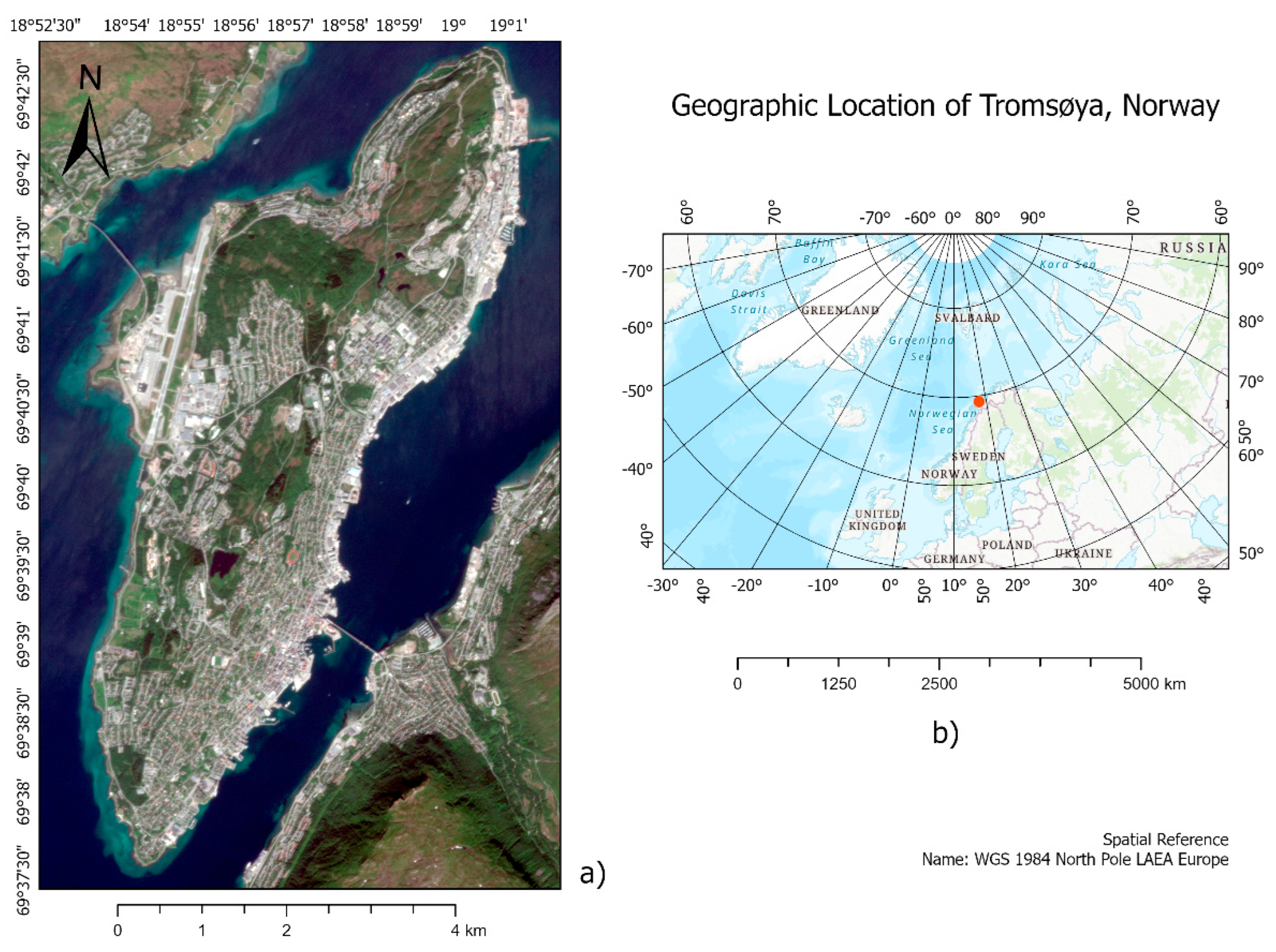
Figure 2.
Per-class meanF1 for models M1, M2, M3 and sensors: (a) Landsat, (b) PlanetScope. The numbers next to the trajectories show the gains: Δ(M2-M1) - the effect of CHM (first value), Δ(M3-M2) - the additional effect of OSM (second value).
Figure 2.
Per-class meanF1 for models M1, M2, M3 and sensors: (a) Landsat, (b) PlanetScope. The numbers next to the trajectories show the gains: Δ(M2-M1) - the effect of CHM (first value), Δ(M3-M2) - the additional effect of OSM (second value).
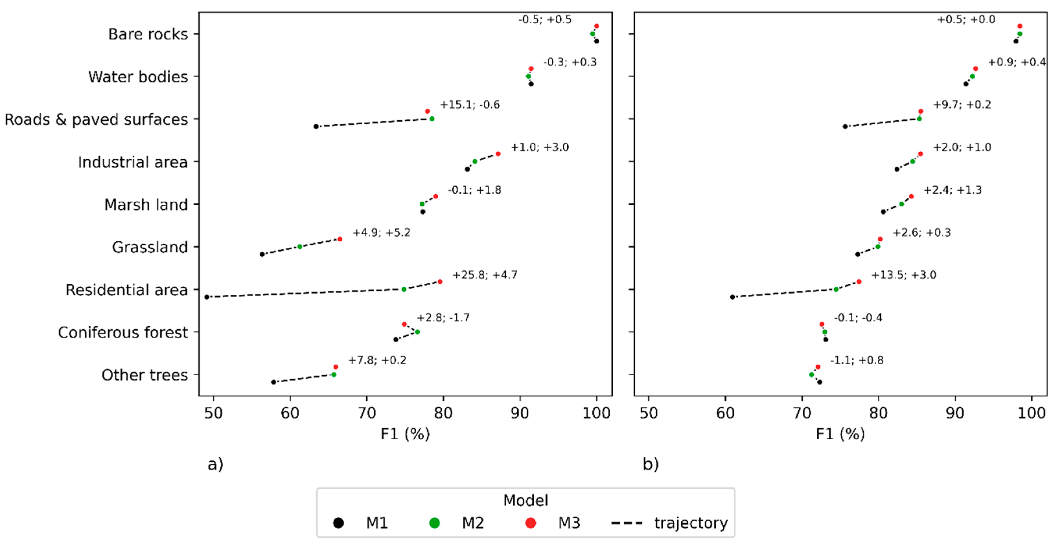
Figure 3.
Averaged class-to-class misclassification (% of true class) by sensor and models.
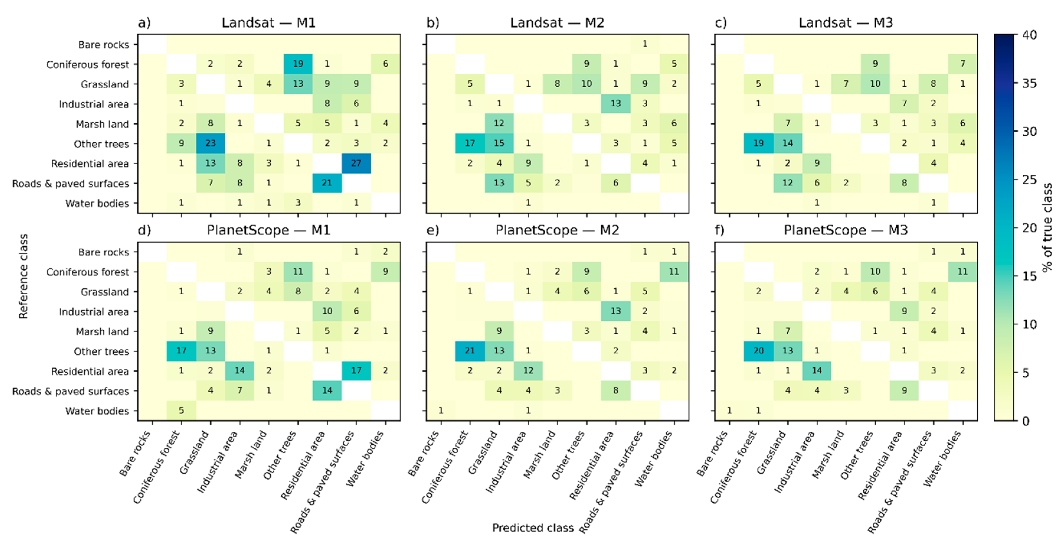
Figure 4.
Visual comparison of LULC (2024) based on PlanetScope (a, b, c) and Landsat (d, e, f) and models with an emphasis on the interpretation of class-wise classification improvements.
Figure 4.
Visual comparison of LULC (2024) based on PlanetScope (a, b, c) and Landsat (d, e, f) and models with an emphasis on the interpretation of class-wise classification improvements.
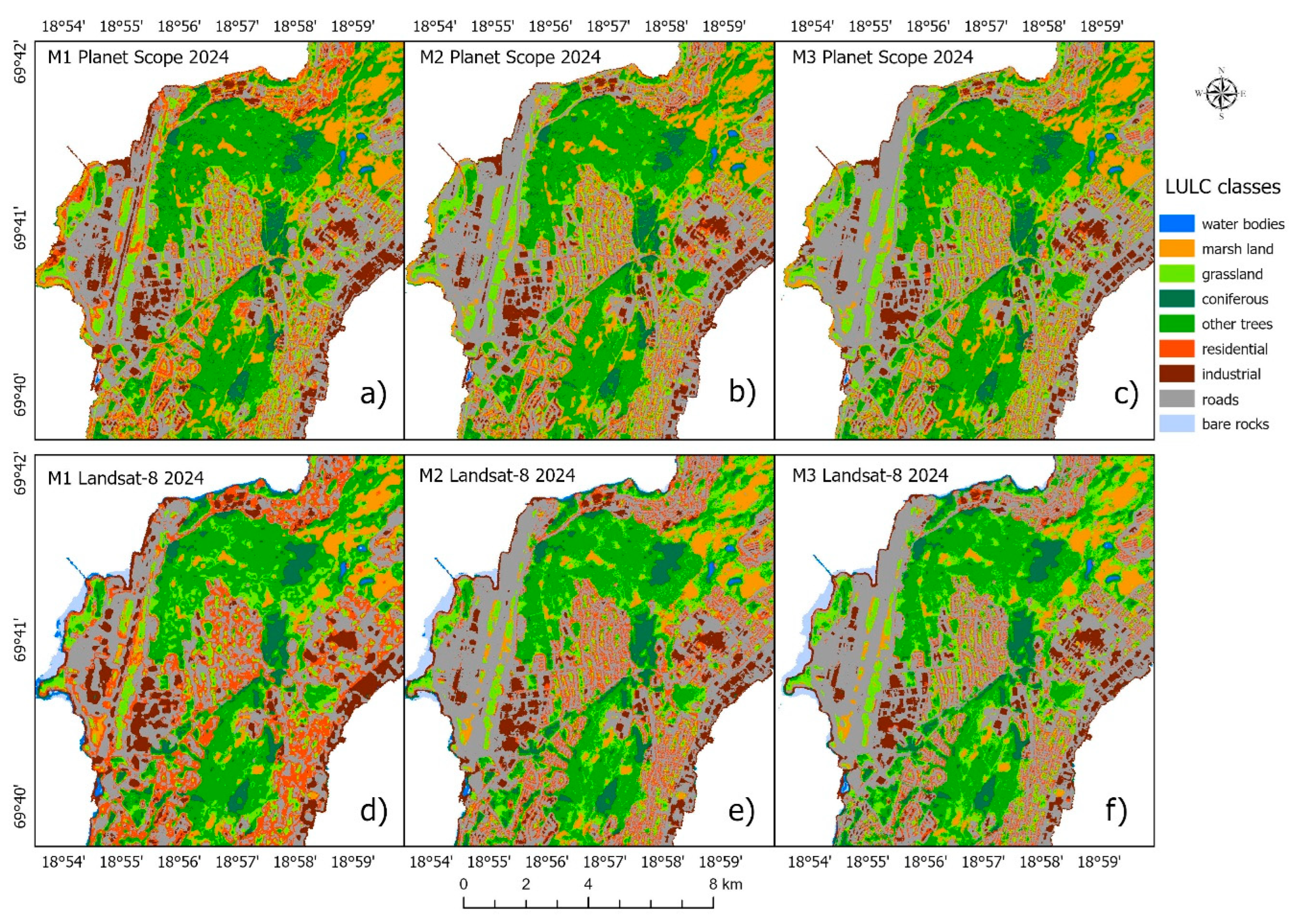
Figure 5.
Cross sensor agreement in class areas for the overlap years 2017, 2020, and 2024 based on M3. (a) Per class area differences (Δ = Landsat minus PlanetScope, km²). Summary dispersion statistics across the three years: the median absolute deviation (MAD) and the sample standard deviation (SD); (b) Normalised transition matrix (mean of 2017, 2020, 2024) showing class to class area reallocations from Landsat (rows) to PlanetScope (columns), expressed as a percentage of the Landsat class area.
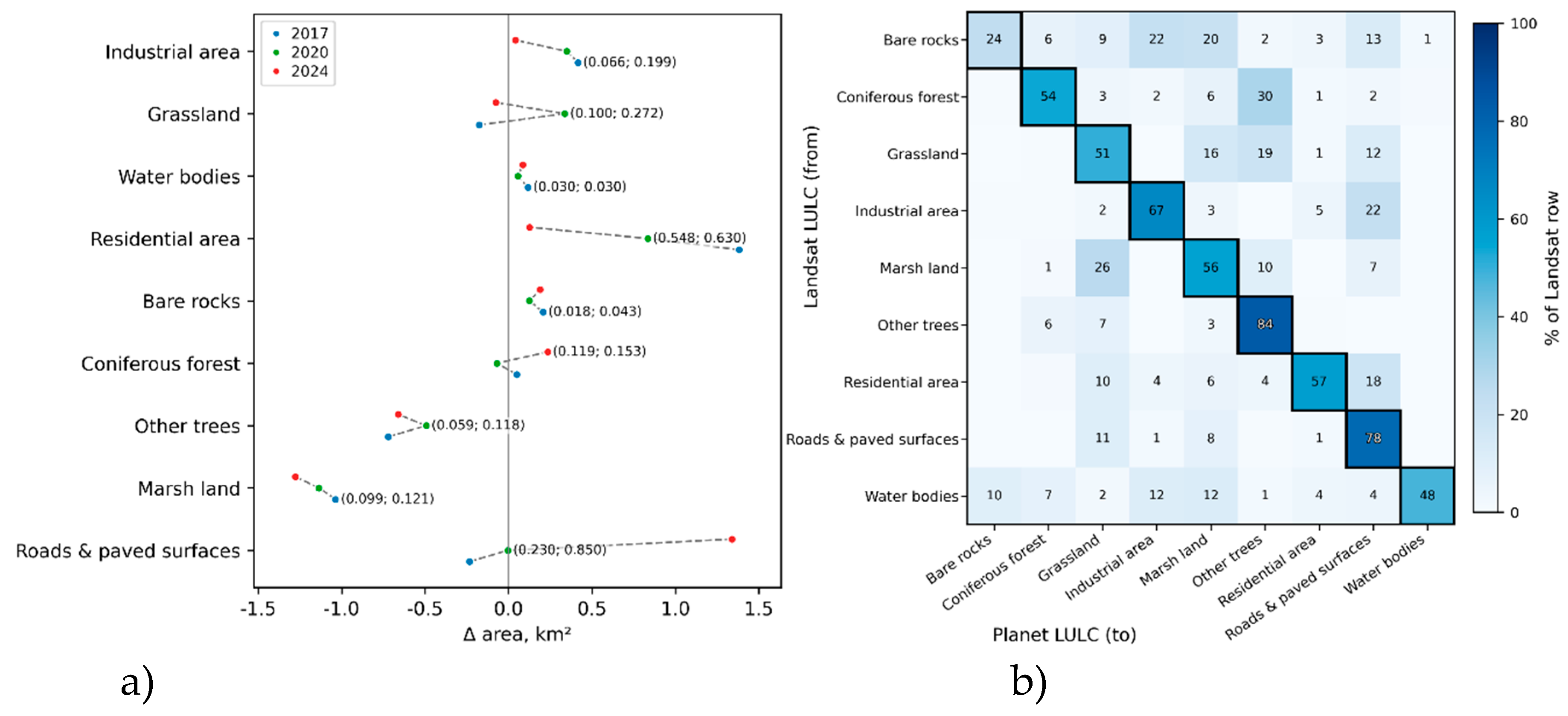
Figure 6.
The diagram depicts the dynamics of transitions between LULC classes for the control years based on Landsat. Each vertical column shows the composition of class areas in the corresponding year (segment height is proportional to class area, km² and the scale is normalised). Smooth ribbons between adjacent columns represent transitions between classes. The ribbon thickness is proportional to the transition area (%). A duplicate 1984 column is added on the right to separately display direct transitions from 1984 to 2024. Within-column labels report class areas (%) for substantive segments and totals per year are shown above each column. Very small flows have been filtered out (threshold = 0.30) to improve readability.
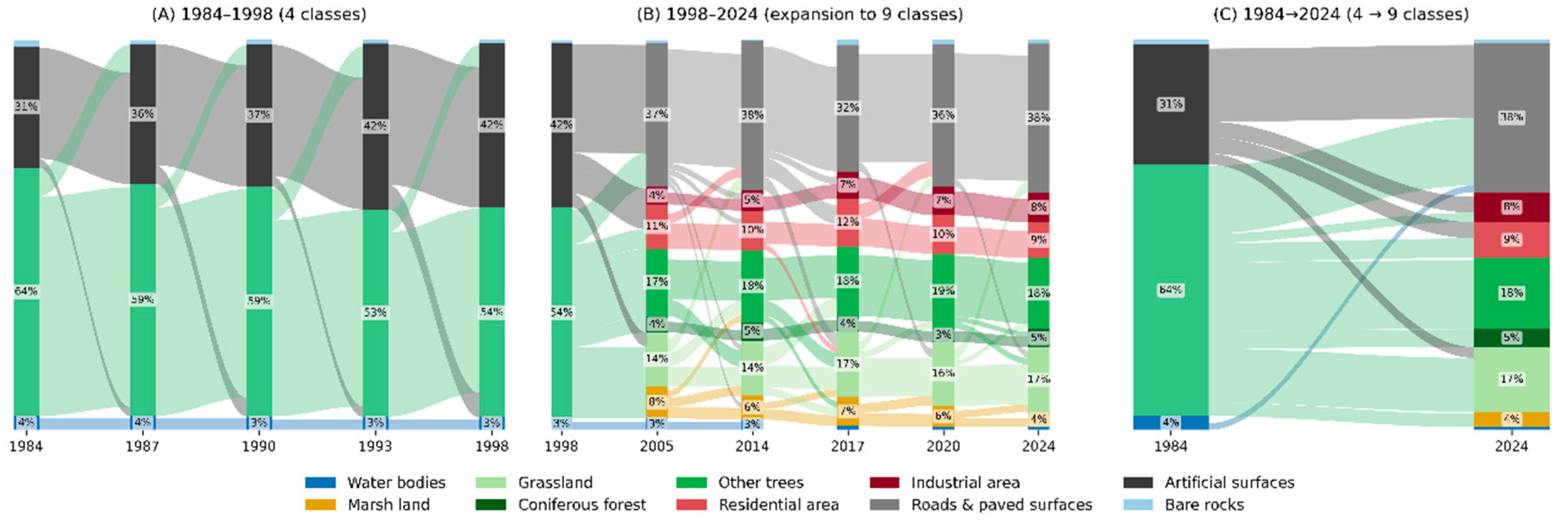
Figure 7.
Spatial expression of long term land cover change on Tromsøya between 1984 and 2024 based on Landsat M3: a) categorical change map highlighting locations where green surfaces in 1984 were converted to artificial surface classes by 2024; b) LULC map for 2024 using the expanded nine class scheme (water bodies, marsh land, grassland, coniferous forest, other trees, residential area, industrial area, roads and paved surfaces, bare rocks). c) LULC map for 1984 using the aggregated four class scheme (water bodies, green surfaces, artificial surfaces, bare rocks).
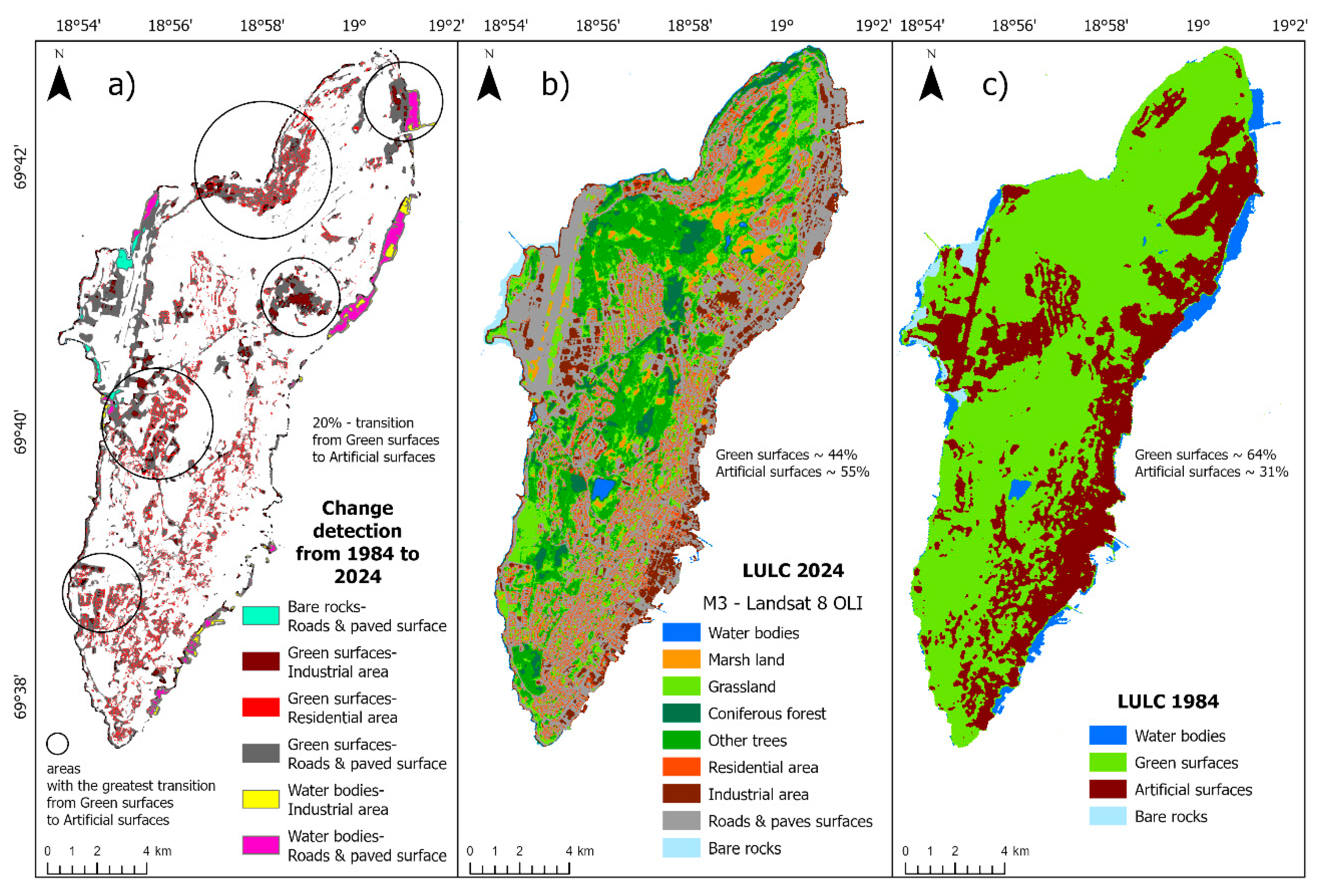
Figure 8.
Population redistribution across districts and change in the balance between green and artificial surfaces on Tromsøya. Embedded bar charts summarise the proportion of green versus artificial surfaces for 1984 and 2024 within each district based on Landsat M3.
Figure 8.
Population redistribution across districts and change in the balance between green and artificial surfaces on Tromsøya. Embedded bar charts summarise the proportion of green versus artificial surfaces for 1984 and 2024 within each district based on Landsat M3.
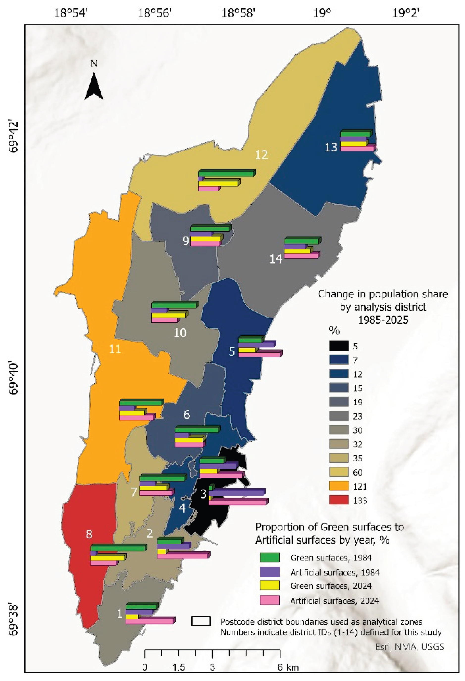

Table 1.
LULC classification performance by year and sensor (Landsat, PlanetScope). BA (%) for models M1, M2, M3 (Equation 1-3).
Table 1.
LULC classification performance by year and sensor (Landsat, PlanetScope). BA (%) for models M1, M2, M3 (Equation 1-3).
| ΔOSM | ΔCHM | BA, % | Sensor | Year | ||
|---|---|---|---|---|---|---|
| M3 | M2 | M1 | ||||
| 1.22 | 8.52 | 81.96 | 80.74 | 72.22 | Landsat | 2024 |
| 1.15 | 3.32 | 85.43 | 84.28 | 80.96 | Planet | |
| 1.8 | 6.47 | 79.56 | 77.76 | 71.29 | Landsat | 2020 |
| 0.94 | 2.86 | 82.05 | 81.11 | 78.25 | Planet | |
| 1.16 | 3.77 | 78.33 | 77.17 | 73.4 | Landsat | 2017 |
| 0.02 | 4.15 | 82.15 | 82.13 | 77.98 | Planet | |
| 6.99 | 75.81 | 68.82 | Landsat | 2014 | ||
| 6.48 | 72.89 | 66.41 | Landsat | 2005/06 | ||
Disclaimer/Publisher’s Note: The statements, opinions and data contained in all publications are solely those of the individual author(s) and contributor(s) and not of MDPI and/or the editor(s). MDPI and/or the editor(s) disclaim responsibility for any injury to people or property resulting from any ideas, methods, instructions or products referred to in the content. |
© 2025 by the authors. Licensee MDPI, Basel, Switzerland. This article is an open access article distributed under the terms and conditions of the Creative Commons Attribution (CC BY) license (http://creativecommons.org/licenses/by/4.0/).
Copyright: This open access article is published under a Creative Commons CC BY 4.0 license, which permit the free download, distribution, and reuse, provided that the author and preprint are cited in any reuse.


