
Submitted:
19 December 2025
Posted:
22 December 2025
You are already at the latest version
Abstract
We investigate the oscillatory behavior of a first-order difference equation with several advanced arguments. New sufficient conditions for oscillation are established, and we show, through carefully constructed counterexamples, that many well-known criteria for equations with a single advanced argument fail to generalize to the several-argument setting, even when each advanced argument is increasing. Several illustrative examples are also provided to demonstrate the sharpness and practical effectiveness of the obtained con- ditions and to highlight their clear improvements over all existing results in the literature
Keywords:
difference and differential equations
; oscillation
; several nonmonotone advanced arguments
1. Introduction
Consider the first-order difference equations with several advanced arguments
where denotes the set of positive integers and is the backward difference operator. Throughout the paper, the coefficient sequences , , are assumed to be nonnegative real-valued for all sufficiently large n. Moreover, the integer-valued sequences represent advanced arguments and satisfy
A sequence , for some , is said to be a solution of equation (1) if it satisfies the equation for all .
The oscillation theory of differential and difference equations provides fundamental insights into the qualitative behavior of dynamical systems across diverse domains, including population dynamics, control systems, biological feedback or feedforward mechanisms [24,31], neural modeling [30,33], and economics, see [2,23,28,29]. The analysis of oscillatory behavior enables researchers to determine whether solutions fluctuate around equilibrium states or converge monotonically, thereby revealing underlying stability properties, periodic tendencies, or chaotic dynamics in physical and biological processes. In discrete systems, oscillation analysis assumes particular significance, as many real-world models evolve through discrete time steps and incorporate delay or advance arguments to capture memory effects or anticipation mechanisms, see [2,23].
The study of oscillation in difference equations plays an essential role in discrete mathematics, and its development has been addressed in a wide range of contributions; see [2,3,4,5,6,7,8,9,10,11,12,13,14,15,16,18,19,20,22,23,25,26,27,32,34,35,36,37]. While classical results typically assume single monotone arguments, realistic systems often involve several advanced arguments that may vary non-monotonically over time. Such complex structures arise naturally in predictive control systems, biological population models with anticipation mechanisms, and signal propagation through feedback networks [10,20,31].
Ladas [27] investigated the oscillatory behavior of the first-order differential equation with non-decreasing delay
and established the well-known lim sup-type oscillation criterion
Motivated by the continuous case, Chatzarakis and Stavroulakis [21] extended Ladas’ condition to the discrete setting. In particular, they obtained the following discrete analogue of (2):
for the advanced difference equation
where is a sequence of nonnegative real numbers and is an integer-valued non-decreasing sequence satisfying
Subsequently, Chatzarakis, Pinelas, and Stavroulakis [14] extended condition (3) to Eq. (1) and obtained
where and each represents a non-decreasing sequence.
Braverman and Karpuz [9] demonstrated that condition (2) is not valid for both the continuous and the corresponding discrete cases when the assumption of monotonicity is relaxed to allow for general, not necessarily monotone, delay arguments. This finding highlights the limitations of directly extending results from monotone to non-monotone delays and shows that more specific methods are required for equations with non-monotone arguments [25,26].
Despite notable progress in the oscillation theory of delay difference equations, the case involving several advanced arguments remains insufficiently explored. Existing studies [1,9] present only sufficient conditions for the oscillation of all solutions; however, they do not reveal the qualitative differences between equations with one or with several advanced arguments. Following the approach in [9], we construct a counterexample showing that some extensions of condition (3) cannot hold for Eq. (1), even when the advanced arguments are non-decreasing and satisfy . In this work, we show that there is no constant such that any of the following conditions guarantees the oscillation of all solutions of Eq. (1):
or
This paper has two additional goals. First, we develop a new framework for studying oscillatory behavior and obtain new sufficient conditions that extend and unify earlier results (see Table 1 on page 7). Second, we show that, for a certain class of equations of the form (1), some of our criteria guarantee oscillation, while all previously known conditions, whether iterative or not, fail for this class. Finally, we introduced a new concept for difference equations with advanced arguments, namely, the distance between generalized successive zeros of solutions, illustrated through numerical simulations.
2. Main Results
Theorem 1.
None of the following conditions, for any constant , guarantees the oscillation of Eq. (1) when is non-decreasing for all and :
- (i)
- (ii)
Proof.
Consider the first–order difference equation with several advanced arguments
It is evident that this equation is a particular case of (1), with
The above equation possesses a non-oscillatory solution
Furthermore, we obtain
and similarly,
As the integer M may be taken arbitrarily large, the proof of the theorem is complete. □
In what follows, and throughout the remainder of this work, we assume that , for , are integer-valued (it is not necessarily assumed to be non-decreasing). Accordingly, we introduce the non-decreasing sequences
Furthermore, for integers , we define
The following lemma provides an iterative sequence of lower bounds for the ratio , which progressively increases as k increases. The proof of this Lemma, for difference equation with several delays, can be found in [10].
Lemma 1.
Assume that is a positive solution of Eq. (1). Then for all , , we have
Proof.
Since the sequence is positive, it follows from Eq. (1) that is eventually non-decreasing. Consequently,
Hence, from (8) we have
That is,
Moreover, since , it follows that
Substituting this estimate into (8) and rearranging the terms yields
Proceeding inductively in this manner, we finally arrive at inequality (7). □
Theorem 2.
(Main oscillation criterion for several non-monotone advanced arguments)
Proof.
Assume, for the sake of contradiction, that Eq. (1) possesses a non-oscillatory solution . Without loss of generality, we may suppose that for all sufficiently large values of n. Hence, is eventually non-increasing for all sufficiently large n.
Summing Eq. (1) from n to , , yields
By virtue of inequality (7) and the fact that for all , it follows that
Substituting this estimate into the previous equality gives
Summing this inequality for , we obtain
Now, according to condition (9), there exists a sufficiently large i such that
Combining this fact with inequality (11) yields a contradiction that completes the proof. □
Theorem 3.
Proof.
It is straightforward to reorder the sequences and , for , associated with Eq. (1), so that the following inequality is eventually satisfied:
Theorem 4.
Proof.
As before, let denote a positive solution of Eq. (1). From Eq. (1), it immediately follows that
Following the same arguments as in the proof of Theorem 2, and using (7) with for all , summing from ℓ to m yields
From this and condition (14), we arrive at a contradiction, which completes the proof of the theorem. □
Remark 1.
It is worth noting that one of the significant consequences of Theorem 1 is that none of the conditions
or
where each denotes a non-decreasing sequence of positive integers, is a necessary condition for the non-oscillation of Eq. (1).
3. Numerical Results and Simulations
In this section, we provide a comparative analysis between our results and those reported in previous studies, as summarized in Table 1. It is clear that all existing works establish only sufficient conditions for the oscillation of Eq. (1). In contrast, our results not only yield new and sharper oscillation criteria but also reveal that certain formulates are not sufficient to ensure the oscillatory behavior of all solutions of Eq. (1).
We also present two numerical examples to demonstrate the validity and sharpness of the obtained results. The first example applies one of the main theorems to show that a class of difference equations of the form (1) is oscillatory, while previously known criteria fail to detect this behavior; several solution simulations and graphical representations further illustrate the oscillatory nature and identify regions where earlier conditions are ineffective. The second example addresses a qualitative property that, to the best of the authors’ knowledge, has not been previously studied for difference equations advanced arguments, namely the distance between generalized zeros, and the simulations indicate that this distance decreases as the sequence of coefficients increases, highlighting the relevance of this property for a deeper understanding of the solution dynamics.
Example 1.
Consider the first-order difference equation with several advanced arguments
where
and
where , and denotes the greatest integer less than or equal to .
Furthermore, , and
where , , and the sequence satisfies
It follows directly that condition (13) holds, and
Consequently, for , we obtain
Therefore, condition (14) is satisfied with , and hence Eq. (17) is oscillatory.
However, as will be demonstrated below, all known iterative and non-iterative oscillation criteria fail to establish the oscillatory behavior of Eq. (17). For example,
where . Therefore,
Consequently, ([14] Theorem 3.2) cannot be applied to Eq. (17). Furthermore, we observe that
and
Moreover, define
Therefore,
and
Similarly,
Consequently,
for sufficiently small and . Hence, [17] (Theorem 2.7) is not satisfied.
Likewise, it can be shown that the remaining oscillation conditions are not satisfied for Eq. (17).
This example demonstrates that condition (14) yields sharper results than existing ones. The numerical results confirm the oscillatory behavior of Eq. (17). As seen in Figure 1, the solution oscillates for and with , while smaller leads to more sign changes, motivating further study of the distance between generalized zeros (see Example 2).
In addition, we illustrate, through several graphical representations, a comparison between condition (14) and [17] (Theorem 2.7). Specifically, we define the function
where . We plot the relationship between and the parameter . As illustrated in Figure 2 and Table 2, the oscillation condition of [17] (Theorem 2.7), for and 3, is not satisfied on the intervals
respectively. However, as shown above, Eq. (17) is oscillatory for all and .
Example 2.
Consider the difference equation with advanced argument
This equation represents a particular case of Eq. (4) with and . Numerical simulations of Eq. (18) reveal a clear dependence between the parameter and the distance between consecutive generalized zeros of the solutions. Here, a generalized zero is a positive integer at which the solution is zero or has a different sign than at the preceding integer. The numerical results show that the maximum interval length T, over which the solution remains positive (or negative), decreases as increases. Specifically, for , the corresponding lengths are and 3, respectively (see Figure 3). These findings highlight the importance of examining the spacing between successive generalized zeros in advanced-type difference equations, as such an analysis provides deeper insight into the qualitative oscillatory dynamics of these equations.
Conclusion
In this work, we obtained new oscillation criteria for first–order difference equations with several, not necessarily monotone, advanced arguments. Our results substantially strengthen and extend the existing results in the literature. Theorem 1 shows that there are fundamental differences between equations with a single advanced argument and those with several advanced arguments. Moreover, the analytical approach presented here is sufficiently flexible to be applied to further qualitative investigations, including the study of the distribution of generalized zero and related properties of difference equations with generalized delays or advanced arguments.
Author Contributions
Conceptualization, M.T.N. and E.R.A.; methodology, M.T.N. and E.R.A.; software, M.T.N. and E.R.A.; validation, M.T.N., E.R.A. and G.E.C.; formal analysis, M.T.N. and E.R.A.; investigation, M.T.N. and E.R.A.; resources, M.T.N. and E.R.A.; data curation, M.T.N. and E.R.A.; writing original draft preparation, M.T.N., E.R.A. and G.E.C.; writing, review and editing, M.T.N., E.R.A. and G.E.C.; visualization, M.T.N. and E.R.A.; supervision, E.R.A.; project administration, E.R.A.. All authors have read and agreed to the published version of the manuscript.
Funding
This research was funded by Prince Sattam bin Abdulaziz University, project number PSAU/2025/01/31196. The Article Processing Charge (APC) was also funded by Prince Sattam bin Abdulaziz University.
Institutional Review Board Statement
Not applicable. This study does not involve human participants or animals.
Informed Consent Statement
Not applicable. This study did not involve human participants.
Data Availability Statement
This is a theoretical study in the field of mathematics. No new data were created or analyzed in this work. Therefore, data sharing is not applicable to this article.
Acknowledgments
The authors extend their appreciation to Prince Sattam bin Abdulaziz University for funding this work through project number (PSAU/2025/01/31196).
Conflicts of Interest
The authors declare no conflicts of interest. The funders had no role in the design of the study; in the collection, analyses, or interpretation of data; in the writing of the manuscript; or in the decision to publish the results.
Abbreviations
The following abbreviations are used in this manuscript:
| DE | Difference Equation |
| NDE | Neutral Difference Equation |
| 1st-order | First-order |
| non-monot. | Non-monotone |
| args. | Arguments |
| e.g. | For example (exempli gratia) |
| i.e. | That is (id est) |
| etc. | And so forth (et cetera) |
| cf. | Compare (confer) |
| lim inf | Limit inferior |
| lim sup | Limit superior |
| w.l.o.g. | Without loss of generality |
| w.r.t. | With respect to |
| resp. | Respectively |
References
- Agarwal, R.P.; O’Regan, D.; Wong, P.J.Y. Positive solutions of differential, difference and integral equations. J. Math. Anal. Appl. 2005, 300, 465–483. [Google Scholar]
- Agarwal, R.P.; Grace, S.R.; O’Regan, D. Oscillation Theory for Difference and Functional Differential Equations; Springer: Berlin, Germany, 2013. [Google Scholar]
- Attia, E.R. New oscillation results for first-order nonlinear difference equations with retarded arguments. J. Math. Comput. Sci. 2024, 32, 241–255. [Google Scholar] [CrossRef]
- Attia, E.R.; Chatzarakis, G.E. Oscillation tests for difference equations with non-monotone retarded arguments. Appl. Math. Lett. 2022, 123, 107551. [Google Scholar] [CrossRef]
- Attia, E.R.; El-Matary, B.M. New aspects for the oscillation of first-order difference equations with deviating arguments. Opusc. Math. 2022, 42, 393–413. [Google Scholar] [CrossRef]
- Attia, E.R.; El-Matary, B.M.; Chatzarakis, G.E. New oscillation conditions for first-order linear retarded difference equations with non-monotone arguments. Opusc. Math. 2022, 42, 769–791. [Google Scholar] [CrossRef]
- Benekas, V.; Garab, Á.; Kashkynbayev, A.; Stavroulakis, I.P. Oscillation criteria for linear difference equations with several variable delays. Opusc. Math. 2021, 41, 613–627. [Google Scholar] [CrossRef]
- Berezansky, L.; Braverman, E. On existence of positive solutions for linear difference equations with several delays. Adv. Dyn. Syst. Appl. 2006, 1, 29–47. [Google Scholar]
- Braverman, E.; Karpuz, B. On oscillation of differential and difference equations with non-monotone delays. Appl. Math. Comput. 2011, 218, 3880–3887. [Google Scholar] [CrossRef]
- Braverman, E.; Chatzarakis, G.E.; Stavroulakis, I.P. Iterative oscillation tests for difference equations with several non-monotone arguments. J. Difference Equ. Appl. 2015, 21, 854–874. [Google Scholar] [CrossRef]
- Chatzarakis, G.E.; Koplatadze, R.; Stavroulakis, I.P. Oscillation criteria of first-order linear difference equations with delay argument. Nonlinear Anal. 2008, 68, 994–1005. [Google Scholar] [CrossRef]
- Chatzarakis, G.E.; Philos, Ch.G.; Stavroulakis, I.P. An oscillation criterion for linear difference equations with general delay argument. Port. Math. 2009, 66, 513–533. [Google Scholar] [CrossRef]
- Chatzarakis, G.E.; Manojlović, J.; Pinelas, S.; Stavroulakis, I.P. Oscillation criteria of difference equations with several deviating arguments. Yokohama Math. J. 2014, 60, 13–31. [Google Scholar]
- Chatzarakis, G.E.; Pinelas, S.; Stavroulakis, I.P. Oscillations of difference equations with several deviated arguments. Aequat. Math. 2014, 88, 105–123. [Google Scholar] [CrossRef]
- Chatzarakis, G.E.; Kusano, T.; Stavroulakis, I.P. Oscillation conditions for difference equations with several variable arguments. Math. Bohem. 2015, 140, 291–311. [Google Scholar] [CrossRef]
- Chatzarakis, G.E.; Jadlovská, I. Improved iterative oscillation tests for first-order deviating difference equations. Int. J. Difference Equ. 2017, 12, 185–210. [Google Scholar]
- Chatzarakis, G.E.; Jadlovská, I. Oscillations in difference equations with several arguments using an iterative method. Filomat 2018, 32, 255–273. [Google Scholar] [CrossRef]
- Chatzarakis, G.E.; Jadlovská, I. Difference equations with several non-monotone deviating arguments: Iterative oscillation tests. Dyn. Syst. Appl. 2018, 27, 271–298. [Google Scholar] [CrossRef]
- Chatzarakis, G.E.; Horvat-Dmitrović, L.; Pašić, M. Oscillation tests for difference equations with several non-monotone deviating arguments. Math. Slovaca 2018, 68, 1083–1096. [Google Scholar] [CrossRef]
- Chatzarakis, G.E.; Pašić, M. Improved iterative oscillation tests in difference equations with several arguments. J. Difference Equ. Appl. 2019, 25, 64–83. [Google Scholar] [CrossRef]
- Chatzarakis, G.E.; Stavroulakis, I.P. Oscillations of difference equations with general advanced argument. Cent. Eur. J. Math. 2012, 10, 807–823. [Google Scholar] [CrossRef]
- Chatzarakis, G.E.; Grace, S.R.; Jadlovská, I. Oscillation tests for linear difference equations with non-monotone arguments. Tatra Mt. Math. Publ. 2021, 79, 81–100. [Google Scholar] [CrossRef]
- Elaydi, S.N. An Introduction to Difference Equations, 3rd ed.; Springer: New York, NY, USA, 2005. [Google Scholar]
- Karatas, M.; Noblet, V.; Nasseef, M.T.; et al. Mapping the living mouse brain neural architecture: Strain-specific patterns of brain structural and functional connectivity. Brain Struct. Funct. 2024, 226, 647–669. [Google Scholar] [CrossRef] [PubMed]
- Karpuz, B. Sharp oscillation and nonoscillation tests for linear difference equations. J. Difference Equ. Appl. 2017, 23, 1929–1942. [Google Scholar] [CrossRef]
- Kitić, N.; Öcalan, Ö. Oscillation criteria for difference equations with several arguments. Int. J. Difference Equ. 2020, 15, 109–119. [Google Scholar]
- Ladas, G. Sharp conditions for oscillations caused by delays. Appl. Anal. 1979, 9, 93–98. [Google Scholar] [CrossRef]
- Li, T.; Frassu, S.; Viglialoro, G. Combining effects ensuring boundedness in an attraction–repulsion chemotaxis model with production and consumption. Z. Angew. Math. Phys. 2023, 74, 109. [Google Scholar] [CrossRef]
- Li, T.; Pintus, N.; Viglialoro, G. Properties of solutions to porous medium problems with different sources and boundary conditions. Z. Angew. Math. Phys. 2019, 70, 1–18. [Google Scholar] [CrossRef]
- Lupinsky, D.; Nasseef, M.T.; et al. Functional magnetic resonance imaging reveals altered functional connectivity associated with resilience and susceptibility to chronic social defeat stress in the mouse brain. Mol. Psychiatry 2025. [Google Scholar] [CrossRef]
- Nasseef, M.T. Measuring Directed Functional Connectivity in Mouse fMRI Networks Using Granger Causality . Doctoral Dissertation, University of Trento, Trento, Italy, 2015. [Google Scholar]
- Pinelas, S.; Dix, J.G. Oscillation of solutions to non-linear difference equations with several advanced arguments. Opusc. Math. 2017, 37, 887–898. [Google Scholar] [CrossRef]
- Soltanpour, S.; Utama, R.; Chang, A.; Nasseef, M.T.; et al. SST-DUNet: Automated preclinical functional MRI skull stripping using smart Swin transformer and dense UNet. J. Neurosci. Methods 2025. [Google Scholar] [CrossRef]
- Stavroulakis, I.P. Oscillations of delay difference equations. Comput. Math. Appl. 1995, 29, 83–88. [Google Scholar] [CrossRef]
- Stavroulakis, I.P. Oscillation criteria for delay and difference equations with non-monotone arguments. Appl. Math. Comput. 2014, 226, 661–672. [Google Scholar] [CrossRef]
- Wu, H.; Dix, J.G. Oscillation of nabla difference equations with several delay arguments. Int. J. Difference Equ. 2019, 14, 179–194. [Google Scholar] [CrossRef]
- Zhang, B.G.; Tian, C.J. Nonexistence and existence of positive solutions for difference equations with unbounded delay. Comput. Math. Appl. 1998, 36, 1–8. [Google Scholar] [CrossRef]
Figure 1.
Discrete oscillatory behavior of the solution for different values of the perturbation parameter with . (A) : The solution exhibits regular oscillations with moderate variation around zero. (B) : The oscillations become more intensive, indicating increased sensitivity to parameter changes. Vertical lines emphasize the discrete character of the sequence, connecting each data point to the abscissa. The distinct oscillatory patterns demonstrate the dependence of the discrete dynamical behavior on the perturbation parameter .
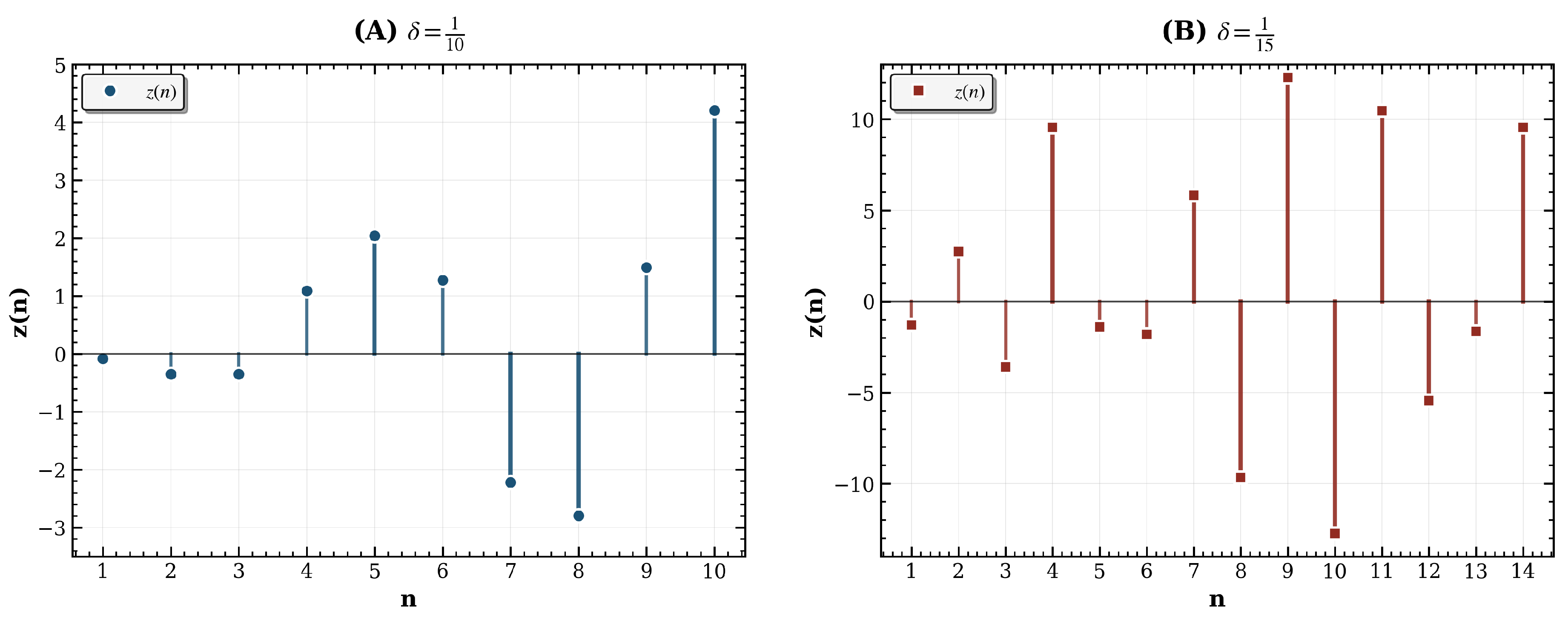
Figure 2.
The curves , , and show the ranges of for which the condition in [17] (Theorem 2.7) holds or fails. It fails from the origin up to the intersection with the horizontal axis and becomes valid thereafter. From the curves, the valid range increases with , reaching its maximum in figure C.
Figure 2.
The curves , , and show the ranges of for which the condition in [17] (Theorem 2.7) holds or fails. It fails from the origin up to the intersection with the horizontal axis and becomes valid thereafter. From the curves, the valid range increases with , reaching its maximum in figure C.
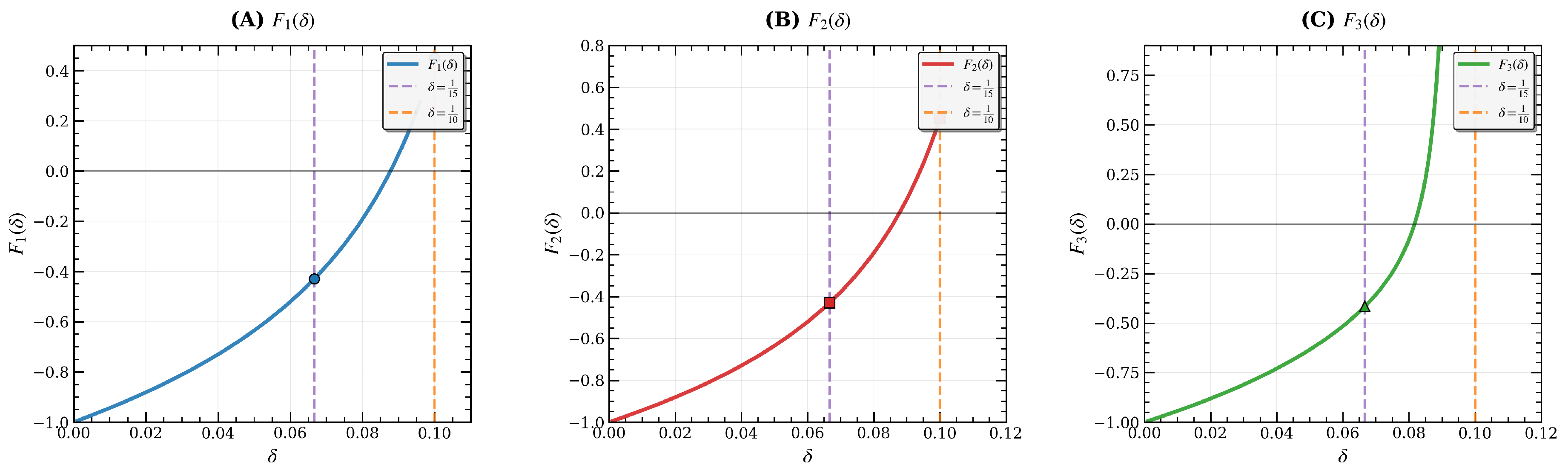
Figure 3.
Discrete oscillatory behavior of the solution of Eq. (18). The four panels display distinct dynamical regimes governed by the parameter . Each discrete value is represented by a colored marker with a vertical line connecting it to the n-axis, emphasizing the discrete nature of the sequence.
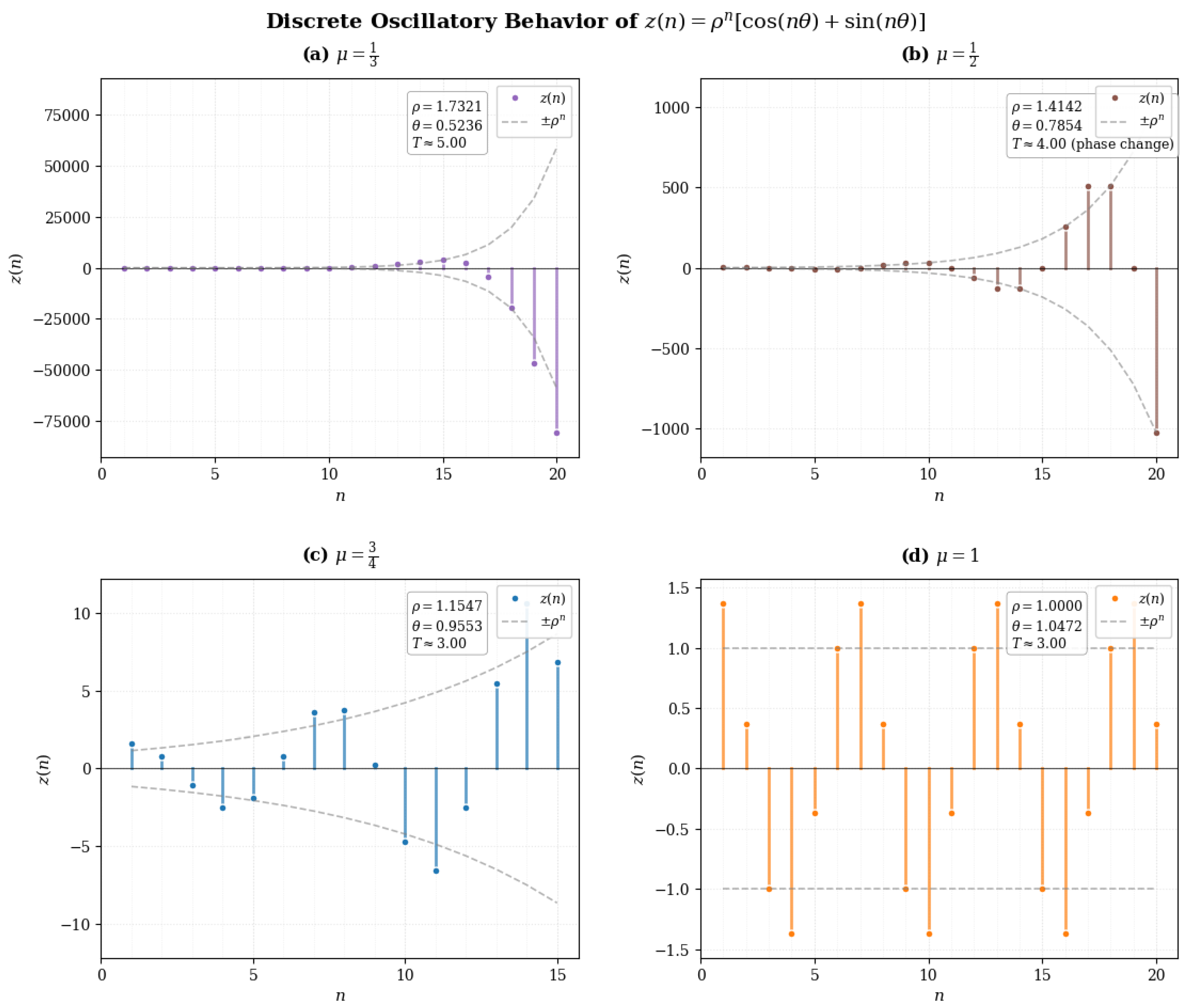

Table 1.
Comparison of existing results with the present study.
| Reference | Type of Equation | Argument Structure | Main Contribution |
|---|---|---|---|
| Braverman & Karpuz (2011) | Delay differential and difference equations | Single nonmonotone delay argument | New oscillation criterion; Monotone-delay results do not extend to non-monotone delay. |
| Chatzarakis et al. [15,18,19,20] | Difference equations with delay and advanced arguments | Several non-monotone arguments | Improved sufficient conditions using summation inequalities. |
| Present study (Nasseef, 2025) | Difference equations with advanced arguments | Several non-monotone advanced arguments | Sharp and generalized oscillation conditions; Monotone-single advanced arguments results can not be extend to several monotone advanced arguments. |
Table 2.
Computed values of the iterative criteria functions , , and for various parameter .
| 0.067 | -0.429338 | -0.286404 | -0.157764 |
| 0.100 | 0.449848 | 0.594833 | 0.754316 |
| 0.020 | -0.881088 | -0.692979 | -0.523681 |
| 0.040 | -0.729753 | -0.556778 | -0.401100 |
| 0.060 | -0.520528 | -0.368476 | -0.231628 |
| 0.080 | -0.191859 | -0.072673 | 0.034594 |
Disclaimer/Publisher’s Note: The statements, opinions and data contained in all publications are solely those of the individual author(s) and contributor(s) and not of MDPI and/or the editor(s). MDPI and/or the editor(s) disclaim responsibility for any injury to people or property resulting from any ideas, methods, instructions or products referred to in the content. |
© 2025 by the authors. Licensee MDPI, Basel, Switzerland. This article is an open access article distributed under the terms and conditions of the Creative Commons Attribution (CC BY) license (http://creativecommons.org/licenses/by/4.0/).
Copyright: This open access article is published under a Creative Commons CC BY 4.0 license, which permit the free download, distribution, and reuse, provided that the author and preprint are cited in any reuse.


