Submitted:
19 December 2025
Posted:
19 December 2025
You are already at the latest version
Abstract
Opinion mining is the process of analyzing the content people create, such as product reviews or social media posts, to determine if the feelings expressed are positive, negative, or neutral. Twitter, one of the most popular social platforms for sharing opinions, provides a lot of data that can be used to understand public sentiment. In this project, we developed a system for classifying sentiments that begins with a detailed preprocessing step using natural language processing techniques. After the data has been processed, the tweets are represented using the traditional Term Frequency-Inverse Document Frequency (TF-IDF) model to highlight the most important text features.To make these features even more relevant, we introduced the Egret Swarm Optimization Algorithm (ESOA), a method for selecting important features inspired by how Great and Snowy Egrets hunt. ESOA uses three strategies—waiting patiently, actively searching, and making decisions based on differences—to find a good balance between exploring new areas and focusing on known ones. This creates a flexible framework that works well in different situations. For sentiment classification, we use a Multi-Head Attention Mechanism (MHAM) that can understand various meanings in user text. We fine-tuned the model’s settings using the Dwarf Mongoose Optimization (DMO) algorithm, along with a strategy that helps each part of the attention mechanism focus on different aspects of the text. Testing our approach on the Sentiment140 dataset shows it works very well, achieving almost 97% accuracy, which is better than other methods that usually reach between 92% and 95%.
Keywords:
feature selection optimization
; multi-head attention
; sentiment analysis
; social media analytics
; swarm intelligence
1. Introduction
Sentiment analysis has become a vital part of modern data analysis, helping organizations and researchers understand public opinions shared across digital platforms. With increasing use of social media, people regularly express their views about products, services, events, and other topics, making platforms like Twitter a valuable source of short, real-time textual data. However, analyzing these user-generated posts is challenging due to the informal writing style, noise, inconsistent grammar, emojis, abbreviations, and limited context typically found in tweets.
Many studies have explored sentiment analysis using machine learning and deep learning frameworks. Traditional approaches often rely on manually engineered features, which limits their ability to generalize across highly dynamic linguistic patterns in social media text. Recent work highlights the need for more robust and scalable systems capable of handling short and noisy content. For example, Carvalho and Plastino [1] demonstrated that the performance of Twitter sentiment models greatly depends on the quality of extracted features, while Kumar and Jaiswal [4] identified shortcomings in conventional soft computing techniques when applied to high-volume Twitter data. Similarly, Pota et al. [6] showed that deep contextual embeddings such as BERT significantly improve sentiment prediction but still face difficulties when handling sparse, high-dimensional input representations.
In addition to feature extraction challenges, optimization of model parameters plays a crucial role in achieving stable and accurate results. Many recent sentiment analysis studies emphasize the importance of utilizing attention mechanisms and neural architectures that can capture semantic nuances in short texts [9,18]. However, these models often struggle with redundant attention focus, suboptimal feature selection, and manually tuned hyperparameters, which introduce instability and reduce overall effectiveness.
To address these limitations, our work proposes a unified sentiment classification framework that integrates advanced natural language processing with hybrid optimization techniques. By incorporating TF-IDF based text representations, the Egret Swarm Optimization Algorithm (ESOA) for feature selection, a Multi-Head Attention Mechanism (MHAM) for semantic learning, and Dwarf Mongoose Optimization (DMO) for hyperparameter tuning, the system aims to overcome the challenges previously highlighted in the literature. The goal is to develop a more efficient and accurate method capable of handling the complexities of Twitter data while leveraging optimization-driven enhancements to improve classification performance.
2. Literature Review
Sentiment analysis on Twitter has been widely studied using various methods, including traditional machine learning techniques, deep learning, and models based on optimization. Earlier work mainly used classic classifiers like Support Vector Machines, Logistic Regression, and Decision Trees. These models had some success but had trouble handling the complex and noisy data found on Twitter. For example, Carvalho and Plastino [1] noted that the effectiveness of these classical models depends heavily on how well the chosen features can distinguish between different sentiments. Similarly, Mehta and Pandya [8] looked at different machine learning methods and found that traditional algorithms aren’t very strong when dealing with informal and quickly changing language on social media. Decision tree-based sentiment classifiers, like those developed by Kasthuri and Jebaseeli [2], provided models that were easier to understand, but they still faced issues with sparse text data and repeated features.
To overcome the problems with manually creating features, researchers started using soft computing and hybrid feature-based approaches. Kasthuri and Jebaseeli [5,7,10] looked into nature-inspired optimization, fuzzy logic, and mixed methods to improve feature selection and classification accuracy. Their findings showed better performance than traditional methods, but these techniques were still sensitive to noisy data and needed a lot of fine-tuning. Kumar and Jaiswal [4] and Kasthuri and Jebaseeli [2] also found that soft computing models worked well but were dependent on high-quality, manually crafted features, which made them hard to use in real-time Twitter settings. Multi-objective optimization models, like the LAN2FIS model introduced by Nagamanjula and Pethalakshmi [14], showed some improvements but came with higher computational costs.
Deep learning became a strong option that can learn meaning patterns directly from text. Models based on LSTM and CNN have shown big improvements, especially for short and casual tweets. For example, Kaur and Sharma [16] created a mixed deep learning model that uses different ways to extract features for analyzing consumer opinions. Krishna et al. [17] used independent component analysis to improve sentiment classification using deep learning. Yin et al. [18] introduced the DPG-LSTM model, which uses dependency parsing and graph convolution to understand both sentence structure and meaning in social media text. These studies showed that deep learning models are better than traditional methods, but they still face challenges like dealing with large amounts of data, messy information, and complicated settings.
Transformer-based models took the field even further by using contextual embeddings. Pota et al. [6] made a BERT-based system for analyzing sentiment on Italian tweets, and it worked well because BERT can understand relationships between words in context. Naseem et al. [9] used transformer-based embeddings that are smart and context-aware, which helped improve accuracy and make models more reliable for sentiment tasks. Wankhade and Rao [21] made a BERT-BiLSTM model that works well for analyzing sentiment about COVID-19, showing how combining transformer embeddings with recurrent models helps handle short and specialized tweets. Azzouza et al. [15] built on this by creating TwitterBERT, a system designed specifically for the types of text found in tweets.
Alongside progress in neural modeling, researchers have looked into using emojis, emoticons, and other language clues to better understand emotions in text. Ullah and others [23] suggested combining text with emoticons, showing how non-verbal expressions are key for predicting emotions. Rachman [24] showed that using TF-IDF along with logistic regression can work well if emotive symbols are kept. Studies by Manguri et al. [3] and Neogi et al. [11] also found that using language patterns specific to certain areas can greatly improve emotion analysis, especially in areas like tracking public health responses to COVID-19 and studying social movements.
There’s also been interest in optimization-based sentiment models, especially for choosing the best features and adjusting model settings. Kasthuri and Jebaseeli [2] introduced a mixed optimization method, showing how nature-inspired techniques can help pick the best features. In stock market prediction, Albahli et al. [19] used machine learning on real-time Twitter data, stressing the need to fine-tune model settings for consistent results. Tesfagergish et al. [20] developed a zero-shot learning method for detecting emotions using sentence transformers and group learning techniques, showing that optimization methods are becoming more important in analyzing text.
In this varied collection of work, a few common issues keep showing up. Many current models have trouble with messy or repeated features, lack of different meanings in their attention systems, and depend too much on manually adjusted settings. While deep learning and transformer models have better ways of representing data, they still don’t perform well if problems like repeated or unstable features aren’t fixed. These shortcomings show that we need a combined approach that includes better ways to pick features, improved attention mechanisms, and automatic tuning of settings—this is why the ESOA-MHAM-DMO model was developed in this study.
3. Problem Statement & Objecctives
3.1. Problem Statement
Sentiment analysis of Twitter data is essential for understanding public opinion across various domains such as product reviews, social events, and policy discussions. However, effective sentiment classification remains a challenging task due to several inherent characteristics of Twitter data. Tweets are often short, noisy, and written in informal language, frequently containing abbreviations, misspellings, emojis, hashtags, and inconsistent grammatical structures. These features make it difficult for traditional sentiment analysis models to accurately capture meaningful contextual and emotional information.
Existing machine learning and deep learning approaches commonly rely on high-dimensional text representations, such as TF-IDF, which often include redundant and irrelevant features. This leads to increased computational complexity and degraded classification performance. Additionally, many deep learning models employ attention mechanisms that tend to focus on overlapping semantic regions, limiting their ability to capture diverse sentiment cues present in short text sequences. Another major limitation observed in current approaches is the dependence on manually selected hyperparameters, which leads to unstable model performance and poor generalization across datasets.
Although recent studies have introduced optimization algorithms and advanced neural architectures, they often address feature selection, attention mechanisms, or hyperparameter tuning in isolation. A unified framework that simultaneously reduces feature redundancy, enhances semantic representation, and optimizes training parameters is still lacking. These challenges motivate the need for an integrated and optimized sentiment classification model capable of handling the complexity and variability of Twitter data more effectively.
3.2. Objectives of the Study
The goal of this research is to develop a strong and efficient sentiment analysis system for Twitter data by combining feature selection, deep learning, and optimization techniques. The specific aims of this study are as follows:
- To create an effective preprocessing and feature extraction process that transforms raw Twitter text into meaningful numerical data while retaining sentiment information.
- To apply the Egret Swarm Optimization Algorithm (ESOA) for selecting relevant and non-redundant features from high-dimensional TF-IDF representations, thereby reducing computational complexity and enhancing classification accuracy.
- To build a sentiment classification model utilizing a Multi-Head Attention Mechanism (MHAM) that captures diverse semantic patterns and improves the contextual understanding of short Twitter messages.
- To optimize the hyperparameters of the deep learning model using Dwarf Mongoose Optimization (DMO) in order to improve training stability and overall performance.
- To evaluate the effectiveness of the proposed framework using the Sentiment140 dataset and compare its performance with existing sentiment analysis approaches based on standard evaluation metrics.
4. Proposed System
The system suggested uses a complete method for analyzing emotions in tweets. It aims to correctly sort the tweets by using natural language processing, better ways to pick important features, and deep learning to classify the sentiment. The process begins with getting the data ready, then cleaning and preparing the text. After that, features are taken out using TF-IDF. The most helpful features are then picked using the Egret Swarm Optimization Algorithm (ESOA). Finally, the sentiment is determined using a Seq2Seq model with a Multi-Head Attention Mechanism (MHAM). The best settings for the model are fine-tuned using the Dwarf Mongoose Optimization (DMO) algorithm.
4.1. Dataset Description for Sentiment140
The Sentiment140 dataset is created by collecting tweets from twitter.com and is commonly used for large-scale sentiment analysis research. Each tweet is automatically labeled based on the emoticons found within the text, eliminating the need for manual labeling. Positive sentiment is identified using emoticons like :), while negative sentiment is identified using :(.
The dataset consists of six attributes:
- Tweet polarity
- Tweet ID
- Date
- Query
- Username
- Tweet text
In this study, only the tweet ID, tweet text, and polarity attributes are used. Sentiment labels are encoded as 0 for negative sentiment and 4 for positive sentiment. The dataset includes 1,600,000 labeled tweets, split evenly into 800,000 positive and 800,000 negative examples. When looking at how the tweets are structured, the longest one has 110 words, but the average length is around 14 words.

Table 1.
Sample Instances from the Sentiment140 Dataset.
| Tweet ID | Tweet Text | Polarity |
|---|---|---|
| 1467810672 | feels cheated out of the ability to text Facebook status updates | 0 |
| 1467810917 | @Kenichan Numerous times, I dove for the ball | 0 |
| 1467824967 | No jobs = no income. How the hell is the minimum wage | 0 |
| 2065732947 | @KateHope thanks for having my back Haha | 4 |
| 2065733289 | Finally home and getting stuff done before an awesome birthday dinner... | 4 |
| 2065782488 | @DerrenLitten Oh, fantastic, I checked it out while napping | 4 |
All the labeled data is in one file called training.1600000.processed.noemoticon.csv.
To make sure results are consistent, a fixed random seed of 2019 was used. The dataset was split into 80% for training and 20% for testing.
The training part was then divided again, with 90% used for actual training and 10% set aside for validation, without using cross-validation.
All the experiments were run on a system that has 24 CPU cores, 252 GB of RAM, and an NVIDIA GTX 1080Ti graphics card.
4.2. Tweets Pre-Processing
Twitter text tends to be messy because people use casual language, emojis, shortened words, hashtags, and sometimes incorrect grammar. Because of this, we use a detailed process to clean the text before we analyze it for sentiment.
The steps in this process are:
- First, we split the tweets into individual words, making sure to remove extra spaces and punctuation.
- Next, we take out any numbers since they don’t help in determining the sentiment.
- We also remove common words like ’a’, ’the’, ’to’, and ’at’ because they don’t carry much meaning in this context.
- Then, we get rid of punctuation marks that don’t add any real meaning to the text.
- After that, we use a process called stemming, which reduces words to their basic form using the Porter stemming method.
- We also pay special attention to words like ’not’, ’never’, and ’do not’, as they can change the meaning and sentiment of a sentence.
- We use a part-of-speech tagging tool called Apache OpenNLP to identify and keep words that are important for sentiment, especially adjectives.
- Finally, we remove mentions of users, URLs, and retweet symbols, but we keep hashtags by removing the ’#’ symbol so the actual words are still useful.
4.2.1. SentiWordNet-Based Polarity Computation
To quantify sentiment strength, SentiWordNet is used to compute positivity and negativity scores for opinion words.
let: Let:
- P be the set of positive opinion words,
- N be the set of negative opinion words,
- be the positivity score of the word,
- be the negativity score of the word.
The Negative sccore is caluculated as:
where and . The negativity score is multiplied by to map its value into the range .
4.3. Feature Extraction Using Term Weighting TF-IDF
Feature extraction is a key step in sentiment classification, where text is turned into numbers that machine learning models can use. In this study, the Term Frequency–Inverse Document Frequency (TF-IDF) method is used to represent tweets.
Term weighting gives more importance to words that appear often in a document but not too much in other documents. TF-IDF is based on three things: how often a word appears in a single document, how common it is across all documents, and a normalization factor.
Let:
denote the frequency of term j in document i,
denote the number of documents containing termj
N denote the total number of documents.
The TF-IDF weight is computed as:
This approach focuses on highlighting words that carry emotional or meaningful information while removing common words that don’t add much value. However, TF-IDF creates a large number of features, which is why people often use feature selection methods.
4.4. Feature Selection Algorithm: Egret Swarm Optimization Algorithm (ESOA)
The Egret Swarm Optimization Algorithm (ESOA) is a problem-solving method inspired by the behavior of Snowy Egrets and Great Egrets when they look for food. Snowy Egrets usually stay still and wait for prey, while Great Egrets move around actively to find their food. The ESOA operates through three main stages:
- Sit-and-Wait Strategy
- Aggressive Strategy
- Discriminant Condition
In this algorithm, each group of egrets has three members:
- Egret A, which uses a method similar to finding the best path
- Egret B, which randomly explores different areas
- Egret C, which helps bring the group together to focus on the best solution
4.4.1. Sit & Wait Strategy
Let the position of the th i th Egret be:
The observation function is defined as:
The estimation equation is:
The estimation error is calculated as:
The descent direction is obtained as:
Egrets update weights adaptively as:
where = =0.9.
The position update for Egret A is:
4.4.2. Aggressive Strategy
Egret B explores randomly:
Egret C exploits promising regions using encircling behavior:
where .
4.4.3. Discriminant Condition
A discriminant rule selects the best solution:
With a probability of 0.3, inferior solutions may be accepted to avoid premature convergence.
4.4.4. ESOA Pseudocode
| Algorithm 1 Egret Swarm Optimization Algorithm (ESOA) |
|
4.4.5. Computational Complexity
The sit-and-wait strategy needs 11n + 9 floating-point operations, while aggressive strategies need 2n + 2. The discriminant condition needs n operations. Therefore, ESOA has a computational complexity of:
where k is population size and n is feature dimension.
4.5. Classification Using Deep Learning Model
4.5.1. Seq2Seq Model and Attention Mechanism
Given an input tweet sequence:
The encoder hidden state is computed as:
The decoder probability is:
The attention score is computed as:
4.5.2. Multi-Head Attention Mechanism
Encoder states are projected into K semantic spaces:
Context vectors are computed as:
Final context vector:
4.5.3. Penalty Term
To avoid redundancy among attention heads, a penalty term is introduced:
The overall loss function is:
4.5.4. Hyperparameter Optimization
There are a lot of hyperparameters set up for this neural network that need tweaking, and there are some choices that could be debated, like how the data was scaled, if shortcut connections were included, if LSTM layers were used, if two attention layers were added, and if any hidden decisions were missed. Hyperparameter optimization, also called DMO, is done to better understand the model and possibly make it work better. The runtime was improved to 0.01170 seconds using just 41 epochs of training.
4.5.5. Dwarf Mongoose Optimization (DMO) Procedure
Dwarf Mongoose Optimization (DMO) is a stochastic population-based metaheuristic optimization algorithm inspired by the social organization and foraging behavior of the dwarf mongoose (Helogale). In nature, dwarf mongooses exhibit a unique combination of individual food searching and group-based foraging strategies, which enables them to locate optimal food resources efficiently. These animals are semi-nomadic in nature and tend to construct temporary sleeping mounds close to resource-rich regions. The behavioral patterns of dwarf mongooses are statistically modeled in DMO to solve complex optimization problems effectively.
Like other population-based optimization techniques, DMO begins with a random initialization phase, followed by iterative refinement through exploration (diversification) and exploitation (intensification) phases. The convergence towards a global optimum is driven by the collective interactions among the mongooses.
Initialization Phase
The population of candidate solutions is defined as:
where n represents the population size, and each candidate solution is a vector of dimension d.
Each candidate solution is initialized randomly within predefined lower and upper bounds using:
where represents the position of the mongoose in the dimension, and denote the minimum and maximum permissible values, and is a uniformly distributed random number in the interval .
At each step, the solution with the highest fitness value is chosen as the best solution so far.
DMO has two main stages. The first is called Exploitation, where individual mongooses search for better solutions in areas they are already familiar with. The second is called Exploration, where they search randomly to find new food sources or new resting spots. These two stages are handled by three groups within the DMO: the alpha group, the scout group, and the babysitter group.
Unifrnd is a random number that is spread out evenly within a specific range.
VarMin and VarMax are the minimum and maximum values allowed for the problem, and VarSize is the number of data points in the dataset.
In each round, the best solution found so far is retained as the best one.
The DMO, like other metaheuristic algorithms, has two main parts: exploitation, where each individual mongoose focuses on improving its current solution, also known as intensification, and exploration, where a random search is done to find a new food source or a new resting spot, also referred to as diversification.
These two processes are managed by the DMO’s three main social groups: the alpha group, the scout group, and the babysitters.
Choosing the leading female () in a family unit uses Equation (26):
The value represented by n minus b corresponds to the number of mongooses in the top tier. You can think of b as the number of nannies, and peep as the female alpha who calls out directions to the rest of the group. The amount of food available, shown in Equation (27), is what finally determines how the sleeping mound looks.
After each iteration, the position update is calculated using Equation (28), where is a random number that is evenly spread out between and :
When a new sleeping mound is discovered, the average is calculated with the help of Eq. (29):
Once the conditions for changing babysitters are met, the search for the next sleeping spot starts. During this search, they look for a new place that has a different food source. Since mongooses never go back to the same sleeping spot, the group has to keep looking all the time for new ones. In DMO, mongooses often search for food and check out new spots at the same time. This is because the more they travel to look for food, the better chance they have of finding a good new place to sleep.
The scouting update rule is defined by:
Where , and
is a parameter that decreases linearly and controls how much the group of mongooses moves around together.
The vector
represents the force that makes the mongooses move to a new nesting place for the night.
The group responsible for taking care of the young stays with them, while the other mongooses search for a sleeping spot and food. They wait to start foraging or scouting until the babysitting condition in Equation (30) is met, so these members are not counted as part of the total group searching.
Results & Discussion
Confusion Matrix
The effectiveness of a classification model is usually checked using a confusion matrix. This matrix is made from test data where the real class labels are already known. It helps to see how well a classifier is performing by comparing the predicted labels with the actual ones.
As shown in Table 2, there are four different results when classifying a test dataset:
- True Positive (TP): when the model correctly identifies something as positive.
- False Positive (FP): when the model wrongly says something is positive.
- True Negative (TN): when the model correctly identifies something as negative.
- False Negative (FN): when the model wrongly says something is negative.
Table 2.
Confusion Matrix for a Classification Task.
| Actual / Predicted | Predicted Positive | Predicted Negative |
|---|---|---|
| Actual Positive | True Positive (TP) | False Negative (FN) |
| Actual Negative | False Positive (FP) | True Negative (TN) |
Basic Measures Derived from the Confusion Matrix
A confusion matrix serves as the foundation for calculating various quantitative performance metrics. The most commonly used evaluation measures are described below.
Precision:
Precision shows how many of the positive predictions made by a model are actually correct. It looks at the percentage of true positives out of all the positive predictions. When precision is high, it means there are fewer false positives.
Recall (Sensitivity):
Recall, also known as sensitivity, measures the proportion of correctly predicted positive instances among all actual positive instances.
F-Measure:
The F-measure is the harmonic mean of precision and recall and provides a balanced evaluation of the classifier’s performance.
Accuracy:
Accuracy represents the ratio of correctly classified instances to the total number of instances. It is one of the most intuitive performance metrics.
The proposed model achieves an accuracy of 0.8093, indicating that approximately 81% of the test instances are classified correctly.
Figure 1.
Confusion Matrix.
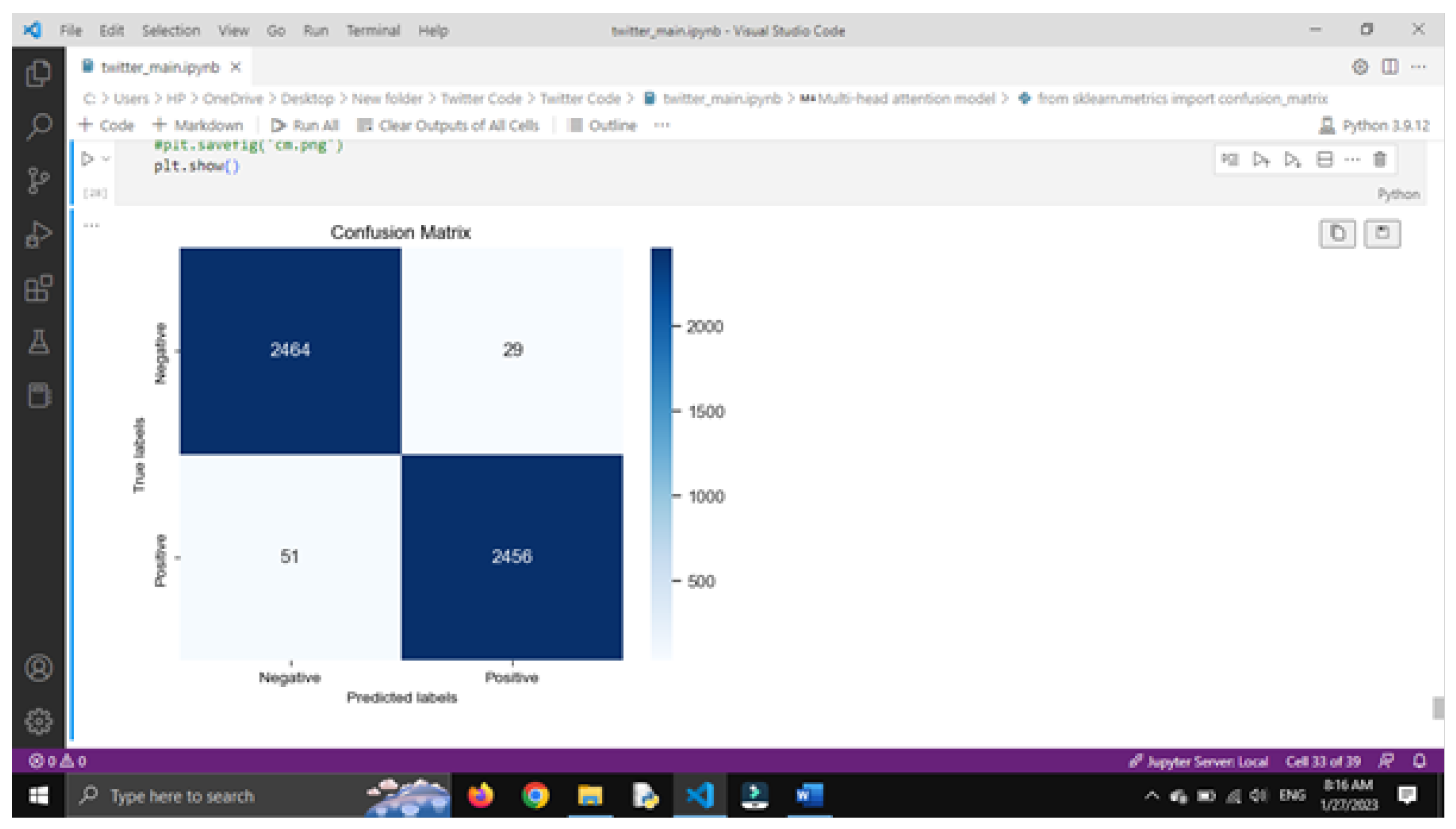
Figure 2 presents the screenshot analysis of proposed model for negative and positive comments.
The accuracy analysis of projected model is exposed in Figure 3
4.6. Performance Analysis of the Proposed Model Without Feature Selection
This section evaluates how effectively the proposed model performs without using the ESOA-based feature selection approach. To ensure a fair comparison, several other models such as LSTM, ICSD, DPG-LSTM, ELM-RNN, BERT-BiLSTM, and SBERT are tested on the same dataset. The average results from these models are then presented. Additionally, traditional machine learning models and standard deep learning models are also included in the testing. The complete comparison results are summarized in Table 3. The results in Table 3 and shown in Figure 4 indicate that the MHAM model works well even without using the ESOA-based feature selection method. Several traditional machine learning models, such as SVM and RF, and different types of neural networks like Auto-encoder, CNN, and LSTM, along with more advanced deep learning models like ICSD, DPG-LSTM, ELM-RNN, BERT-BiLSTM, and SBERT, were tested for comparison.
Among the models tested, SVM and RF achieved accuracy scores of 89.02% and 89.27%, which is quite good. The CNN and LSTM models performed better, with accuracy levels of 92.82% and 90.21% respectively. Transformer-based models, such as BERT-BiLSTM and SBERT, performed even better, reaching accuracy levels of 94.80% and 94.92% respectively.
However, the MHAM model performed the best, achieving an accuracy of 95.20%. It also had better recall, precision, and F-score values compared to all other models. These results show that the MHAM model is very effective for classifying the sentiment of tweets, even without using feature selection, which means it has strong discrimination abilities.
Table 3.
Comparative Performance Analysis of the Proposed Model without ESOA.
| Methodology | Accuracy (%) | Recall (%) | Precision (%) | F-Score (%) |
|---|---|---|---|---|
| SVM | 89.02 | 90.91 | 88.34 | 79.82 |
| RF | 89.27 | 89.27 | 87.72 | 82.20 |
| Auto-encoder | 90.38 | 88.90 | 90.86 | 74.02 |
| CNN | 92.82 | 90.67 | 93.09 | 88.88 |
| LSTM | 90.21 | 92.91 | 93.20 | 83.49 |
| ICSD | 91.20 | 94.04 | 95.90 | 89.90 |
| DPG-LSTM | 92.03 | 95.92 | 95.55 | 91.91 |
| ELM-RNN | 94.44 | 95.64 | 95.30 | 92.04 |
| BERT-BiLSTM | 94.80 | 93.22 | 94.02 | 93.30 |
| SBERT | 94.92 | 94.30 | 96.90 | 94.43 |
| Proposed MHAM | 95.20 | 95.78 | 97.32 | 95.65 |
4.7. Performance Analysis of the Proposed Model with Feature Selection
This part looks at how well the suggested model works when it uses the ESOA-based feature selection method. Like before, the new approach is tested against several traditional machine learning models, deep learning structures, and transformer-based techniques. The results, which include accuracy, recall, precision, and F-score, are shown in Table 4.
Table 4.
Comparative Performance Analysis of the Proposed Model with ESOA.
| Methodology | Accuracy (%) | Recall (%) | Precision (%) | F-Score (%) |
|---|---|---|---|---|
| SVM | 86.12 | 89.94 | 87.38 | 81.85 |
| RF | 87.29 | 88.28 | 88.78 | 86.27 |
| Auto-encoder | 91.88 | 87.95 | 91.87 | 84.42 |
| CNN | 93.42 | 92.68 | 92.12 | 86.89 |
| LSTM | 88.93 | 91.95 | 92.23 | 89.99 |
| ICSD | 89.23 | 92.72 | 92.45 | 89.95 |
| DPG-LSTM | 91.90 | 94.78 | 93.60 | 90.87 |
| ELM-RNN | 94.45 | 94.82 | 94.15 | 91.97 |
| BERT-BiLSTM | 95.46 | 95.55 | 95.80 | 92.54 |
| SBERT | 95.88 | 95.27 | 95.92 | 93.80 |
| Proposed MHAM-DMO | 97.28 | 97.98 | 98.77 | 96.29 |
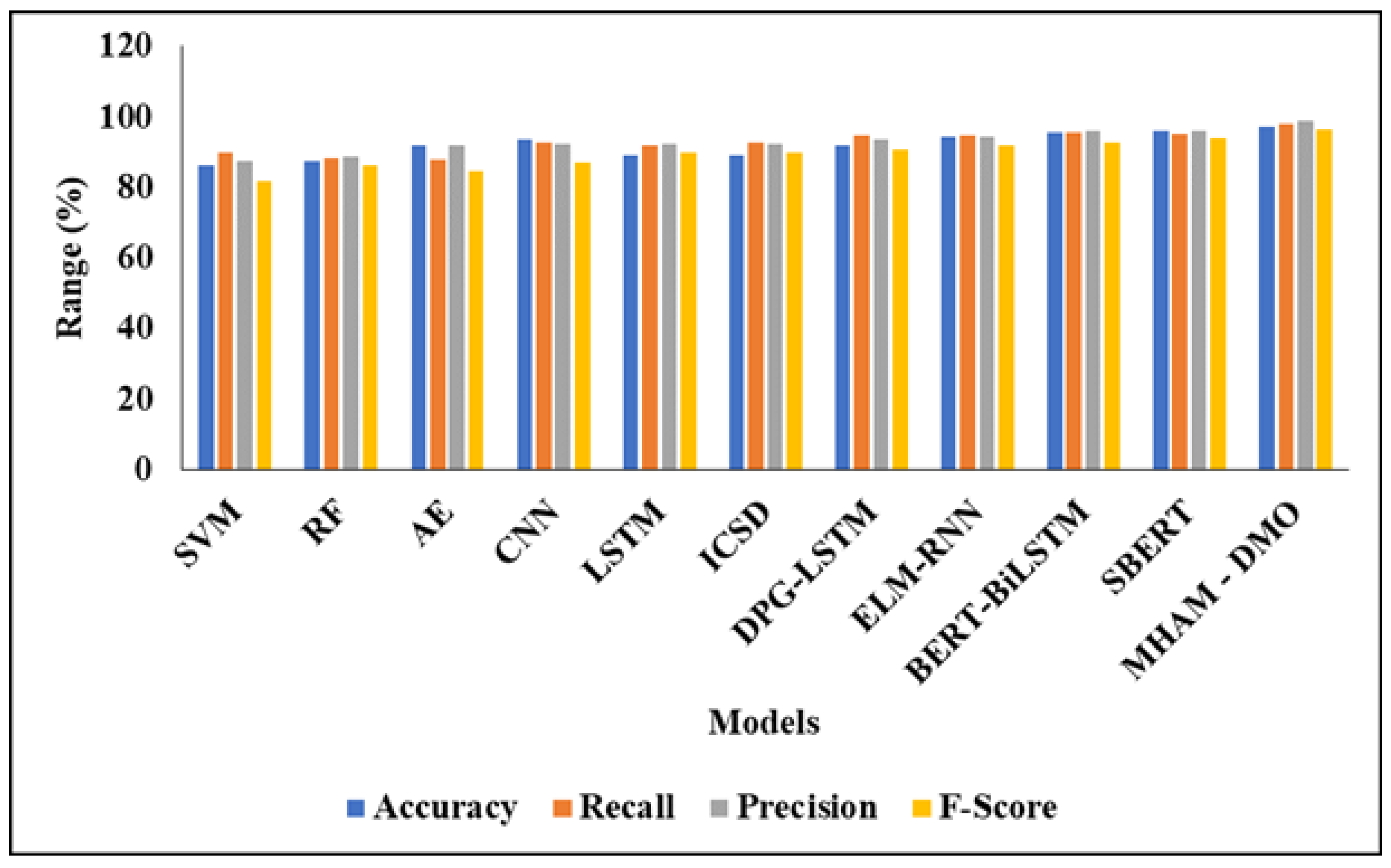
The results in Table 4 and shown in Figure 5 show how using the ESOA-based feature selection method improves the classification results. The test includes traditional machine learning models like SVM and RF, neural networks such as Auto-encoder, CNN, and LSTM, hybrid deep learning models like ICSD, DPG-LSTM, and ELM-RNN, and transformer-based models like BERT-BiLSTM and SBERT.
SVM and RF, which are baseline models, have accuracy scores of 86.12% and 87.29% respectively.
Deep learning models perform better, with CNN reaching 93.42% accuracy. Transformer-based models do even better, with BERT-BiLSTM and SBERT achieving 95.46% and 95.88% accuracy respectively.
The MHAM-DMO model we propose performs the best among all tested methods, with an accuracy of 97.28%, and also has better recall, precision, and F-score.
These results show that combining ESOA-based feature selection greatly improves the model’s ability to distinguish between different classes, surpassing all other methods tested.
5. Conclusion
Sentiment analysis is a way to figure out what people are feeling about a piece of text. It helps us understand their opinions, emotions, and beliefs about something. Both training and testing the models were done using the Twitter dataset. Tweets are short messages with a limit of 140 characters and often include emoticons and emojis. In this study, SentiWordNet is used to group tweets into three categories: positive, negative, or neutral. Using TF-IDF in the feature extraction process led to a big improvement in the accuracy of sentiment analysis. In this research, we present the Egret Swarm Optimization Method, a new meta-heuristic algorithm for feature selection that is inspired by the foraging behaviors of two types of egrets: the Great Egret and the Snowy Egret. The three main ideas behind ESOA are the Snowy Egret’s passive method, the Great Egret’s aggressive approach, and a discriminant illness. To help the decoder give a clear response to an input question, we introduce a DMO with a multi-head attention mechanism. The experimental results show that the proposed model performs better than previous models in terms of classification accuracy. For example, while earlier models had accuracy between 89% and 95% and precision between 88% and 95%, the new model achieved 97.28% accuracy and 98.77% precision. However, there is still a need for a hybrid deep learning model to further improve the study. References
References
- Carvalho, J.; Plastino, A. On the evaluation and combination of state-of-the-art features in Twitter sentiment analysis. Artificial Intelligence Review 2021, 54, 1887–1936. [Google Scholar] [CrossRef]
- Kasthuri, S.; Jebaseeli, N. An Artificial Bee Colony and Pigeon Inspired Optimization Hybrid Feature Selection Algorithm for Twitter Sentiment Analysis. Journal of Computational and Theoretical Nanoscience 2020, 17(12), 5378–5385. [Google Scholar] [CrossRef]
- Manguri, K.H.; Ramadhan, R.N.; Amin, P.R.M. Twitter sentiment analysis on worldwide COVID-19 outbreaks. Kurdistan Journal of Applied Research 2020, 54–65. [Google Scholar] [CrossRef]
- Kumar, A.; Jaiswal, A. Systematic literature review of sentiment analysis on Twitter using soft computing techniques. Concurrency and Computation: Practice and Experience 2020, 32(1), e5107. [Google Scholar] [CrossRef]
- Kasthuri, S.; Jebaseeli, N. Review Analysis of Twitter Sentimental Data. Bioscience Biotechnology Research Communications 2020, 13(6), 209–214. [Google Scholar]
- Pota, M.; Ventura, M.; Catelli, R.; Esposito, M. An effective BERT-based pipeline for Twitter sentiment analysis: A case study in Italian. Sensors 2021, 21(1), 133. [Google Scholar] [CrossRef]
- Kasthuri, S.; Jebaseeli, N. A Robust Data Classification in Online Social Networks through Automatically Mining Query Facts. International Journal of Scientific Research in Computer Science Applications and Management Studies 2018, 7(4). [Google Scholar]
- Mehta, P.; Pandya, S. A review on sentiment analysis methodologies, practices and applications. International Journal of Scientific and Technology Research 2020, 9(2), 601–609. [Google Scholar]
- Naseem, U.; Razzak, I.; Musial, K.; Imran, M. Transformer based deep intelligent contextual embedding for twitter sentiment analysis. Future Generation Computer Systems 2020, 113, 58–69. [Google Scholar] [CrossRef]
- Kasthuri, S.; Jebaseeli, N. An efficient Decision Tree Algorithm for analyzing the Twitter Sentiment Analysis. Journal of Critical Reviews 2020, 7(4), 1010–1018. [Google Scholar]
- Neogi, A.S.; Garg, K.A.; Mishra, R.K.; Dwivedi, Y.K. Sentiment analysis and classification of Indian farmers’ protest using Twitter data. International Journal of Information Management Data Insights 2021, 1(2), 100019. [Google Scholar] [CrossRef]
- Ruz, G.A.; Henríquez, P.A.; Mascareño, A. Sentiment analysis of Twitter data during critical events through Bayesian networks classifiers. Future Generation Computer Systems 2020, 106, 92–104. [Google Scholar] [CrossRef]
- Kasthuri, S.; Jebaseeli, N. Social Network Analysis in Data Processing. Adalya Journal 2020, 9(2), 260–263. [Google Scholar]
- Nagamanjula, R.; Pethalakshmi, A. A novel framework based on bi-objective optimization and LAN2FIS for Twitter sentiment analysis. Social Network Analysis and Mining 2020, 10(1), 34. [Google Scholar] [CrossRef]
- Azzouza, N.; Akli-Astouati, K.; Ibrahim, R. TwitterBERT: Framework for Twitter sentiment analysis based on pre-trained language model representations. In Emerging Trends in Intelligent Computing and Informatics; Springer: Singapore, 2020; pp. 428–437. [Google Scholar]
- Kaur, G.; Sharma, A. A deep learning-based model using hybrid feature extraction approach for consumer sentiment analysis. Journal of Big Data 2023, 10(1), 1–23. [Google Scholar] [CrossRef]
- Krishna, M.M.; Duraisamy, B.; Vankara, J. Independent component support vector regressive deep learning for sentiment classification. Measurement: Sensors 2023, 100678. [Google Scholar] [CrossRef]
- Yin, Z.; Shao, J.; Hussain, M.J.; Hao, Y.; Chen, Y.; Zhang, X.; Wang, L. DPG-LSTM: An Enhanced LSTM Framework for Sentiment Analysis in Social Media Text. Applied Sciences 2023, 13(1), 354. [Google Scholar]
- Albahli, S.; Irtaza, A.; Nazir, T.; Mehmood, A.; Alkhalifah, A.; Albattah, W. A Machine Learning Method for Prediction of Stock Market Using Real-Time Twitter Data. Electronics 2022, 11(20), 3414. [Google Scholar] [CrossRef]
- Tesfagergish, S.G.; Kapočiūtė-Dzikienė, J.; Damaševičius, R. Zero-shot emotion detection for semi-supervised sentiment analysis. Applied Sciences 2022, 12(17), 8662. [Google Scholar] [CrossRef]
- Wankhade, M.; Rao, A.C.S. Opinion analysis during COVID-19 using BERT-BiLSTM ensemble. Scientific Reports 2022, 12(1), 17095. [Google Scholar] [CrossRef] [PubMed]
- Patel, V.; Ramanna, S.; Kotecha, K.; Walambe, R. Short Text Classification with Tolerance-Based Soft Computing Method. Algorithms 2022, 15(8), 267. [Google Scholar] [CrossRef]
- Ullah, M.A.; Marium, S.M.; Begum, S.A.; Dipa, N.S. Sentiment analysis using text and emoticon. ICT Express 2020, 6(4), 357–360. [Google Scholar] [CrossRef]
- Rachman, F.H. Twitter sentiment analysis of COVID-19 using TF-IDF and logistic regression. Proc. 6th Information Technology International Seminar (ITIS), 2020; IEEE; pp. 238–242. [Google Scholar]
Figure 2.
Screenshot Analysis of Proposed model.

Figure 3.
Accuracy Analysis of proposed model.

Figure 4.
Graphical Analysis of Projected model without Feature Selection.
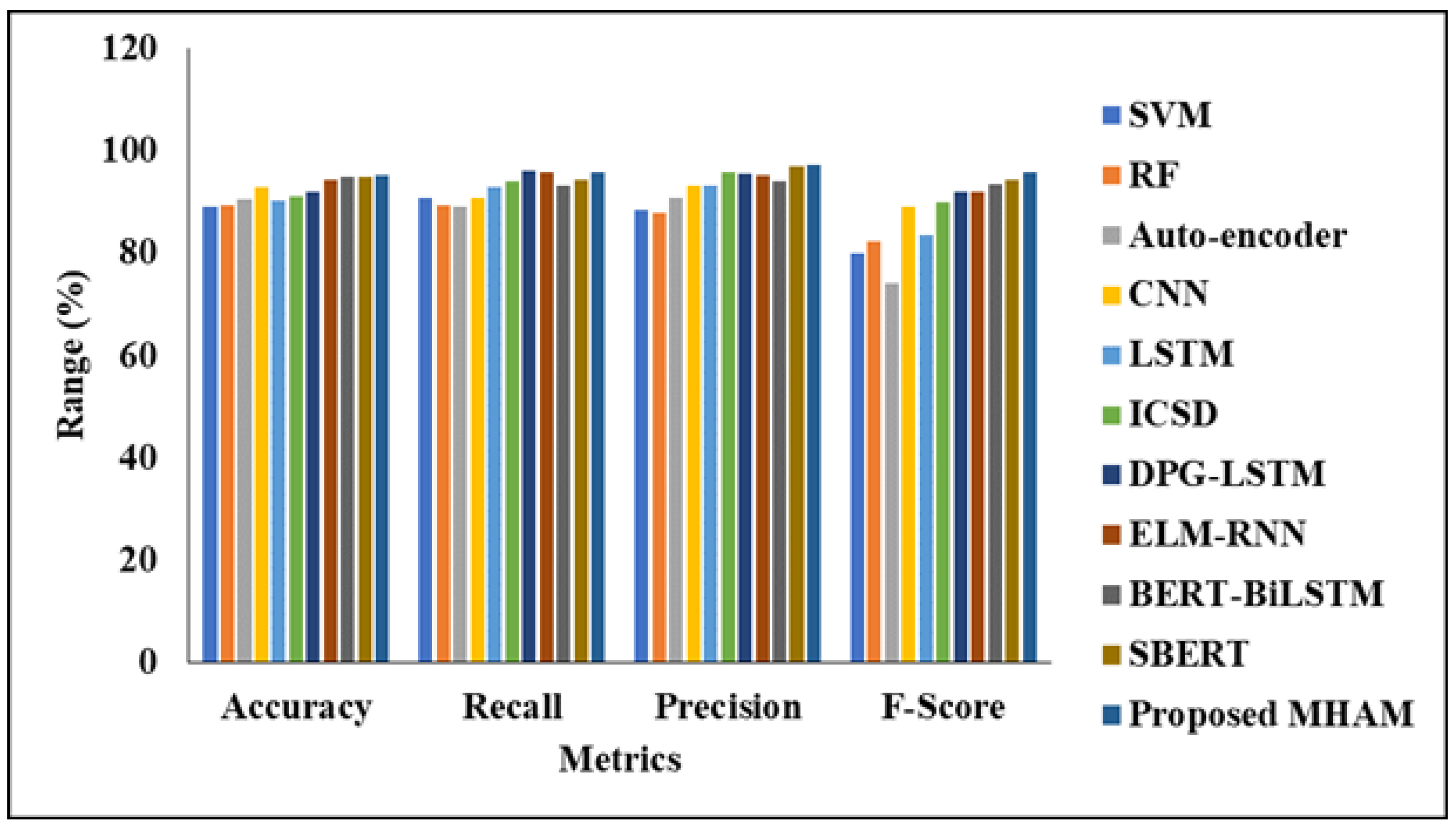
Figure 5.
Graphical Analysis of Projected perfect with Feature Selection.
Disclaimer/Publisher’s Note: The statements, opinions and data contained in all publications are solely those of the individual author(s) and contributor(s) and not of MDPI and/or the editor(s). MDPI and/or the editor(s) disclaim responsibility for any injury to people or property resulting from any ideas, methods, instructions or products referred to in the content. |
© 2025 by the authors. Licensee MDPI, Basel, Switzerland. This article is an open access article distributed under the terms and conditions of the Creative Commons Attribution (CC BY) license (http://creativecommons.org/licenses/by/4.0/).
Copyright: This open access article is published under a Creative Commons CC BY 4.0 license, which permit the free download, distribution, and reuse, provided that the author and preprint are cited in any reuse.


