Submitted:
18 December 2025
Posted:
19 December 2025
You are already at the latest version
Abstract
This project focuses on detecting anomalies in the shipment performance of a Business-to-Business supply chain using machine learning. Two models were used for the analysis: Isolation Forest and One-Class SVM. The model training was conducted using the 2024 data to minimize the impact of COVID-19. The data was cleaned and standardized. The key delivery-performance variables were also created to support more accurate anomaly detection. The Isolation Forest achieved an accuracy of approximately 87% with a 5% contamination factor, while the One-Class SVM achieved an accuracy of approximately 82%. Both models identified the Shipping Point as the primary contributor to delays. When the trained models were tested on the 2025 dataset, Isolation Forest returned more consistent results and captured a wider range of anomalies, including Delivery Delay and quantity shortages (partial deliveries), while the One-Class SVM focused more on timing issues. Overall, the study demonstrated that machine learning–based anomaly detection can help organizations identify delivery issues early and enhance shipment performance in B2B operations.
Keywords:
supply chain analytics
; delivery delay
; lead time
; transit time
; fulfillment gap
; on-time performance
; OTIF
; feature engineering
; data quality assessment
; anomaly detection
; isolation forest
; One-Class SVM
; unsupervised learning
; logistics performance
; operational variability
; early warning indicators
; Dr. Michael McCarthy
Introduction
Timely and consistent delivery performance is one of the most critical indicators of success in business-to-business (B2B) supply chain operations. However, even in highly optimized networks, some orders experience unexpected Delivery Delays that may indicate hidden inefficiencies, disruptions, or risk of cancellation. Traditional approaches to predict the average delay often fail to detect rare or irregular delivery patterns that are significantly different from the norm.
The goal of this research was to identify abnormal delivery behaviors, including extreme delays and irregular delivery patterns. Anomaly detection models were examined and implemented to detect delivery anomalies. The source data spanned from 2020 to 2025; however, to minimize the bias impact of COVID-19 data, the main focus was on the 2024 and 2025 datasets, which reflected current operational trends. The key features impacting delivery performance were identified through Exploratory Data Analysis. The cleaned data, along with the added engineered features, were introduced to the models.
The primary focus of this research was to identify anomalies in delivery timelines using unsupervised machine learning techniques, specifically the Isolation Forest and One-Class SVM algorithms. These anomalies were highlighted as potential inefficiencies or emerging risks for the company.
Fairness, Ethics, Accountability, and Transparency (FEAT) principles should also be considered when interpreting the model results to ensure the models were transparent and aligned with responsible and trustworthy modeling practices. This project presents how anomaly detection models could identify unusual delivery patterns in Business-to-Business (B2B) logistics. The predictions enable the supply chain operations to take early action and improve overall performance.
Literature Review
Many organizations increasingly employ anomaly detection using machine learning to identify outliers and refine their processes to prevent them. The technique is also being used in the supply chain to detect transportation performance issues, inventory disruptions, and Delivery Delays. Numerous research projects have been conducted on such datasets to detect anomalies and improve the delivery performance of supply chains. The foundation for detecting anomalies using machine learning models in this research is based on a literature review of the modern supply chain industry.
Schmidl, Wenig, and Papenbrock (2022) compared 71 anomaly detection algorithms to identify anomalies in a time series of irregularities. They introduce Isolation Forest and Neural Network models as the most effective methods for detecting anomalies. The results of their research align with those of Liu et al. (2008), who also identified anomalies using Isolation Forest as a fast and reliable method for detecting anomalies and outliers. Yokkampon et al. (2021) and Erfani et al. (2016) support the use of the SVM method for large and complex datasets. These findings provide a theoretical basis for selecting the Isolation Forest and One-Class SVM as two strong models for identifying anomalies and outliers in the dataset.
Multiple studies, such as those by Glaser et al. (2022) and Ajeigbe & Moore (2023), also recommend Isolation Forest as a strong model for anomaly detection in supply chain environments.
Khajjou (2023) presents an AI-driven framework to predict anomalies within inventory management systems. Models such as Random Forest, Logistic Regression, and Fast Fourier Transform (FFT) are used to detect anomalous behaviors in supply and demand data, with a focus on backorders, inventory turnover irregularities, and demand seasonality.
Similarly, de Sousa (2022) presents supervised machine learning techniques to predict delayed deliveries with B2B logistics operations. The study is conducted by a European manufacturing firm. The predictive power of Random Forest and Decision Trees is evaluated to identify the best model with the most accurate result.
One-Class Support Vector Machines (SVM) is an algorithm that is recommended in many research studies for anomaly detection in supply chain datasets. Research by Erfani et al. (2016) and Yokkampon et al. (2021) demonstrates that SVM-based models excel on large and complex datasets. Some studies even propose hybrid approaches combining SVM with deep learning to reduce computational complexity and improve accuracy.
Beyond algorithm performance, many papers highlight the broader operational context of anomaly detection. For example, work by Goyal et al. (2023) demonstrates an AI-driven framework for real-time anomaly detection in supply chain resilience. It highlights how anomaly detection models are reducing product waste by 47% and increasing distribution efficiency by 42%.
In supply chains involving items that require refrigeration (i.e., cold chain logistics), studies such as Xie et al. (2025) and Gillespie et al. (2023) demonstrate how environmental factors, including temperature, humidity, and route conditions, affect shipment reliability and can be integrated into anomaly detection models for improved accuracy.
Research also highlights the importance of predicting Lead Times and managing Delivery Delays across various industries. Amellal et al. (2023) and Rokoss et al. (2024) investigate how combining forecasting models, such as Convolutional Neural Networks (CNNs) and Long Short-Term Memory networks (LSTMs), with anomaly detection algorithms can enhance delivery planning. Their findings show that machine learning can reduce forecasting errors and improve the consistency of Lead Time estimation. Other studies, including Shahid (2020) and Mülle et al. (2025), emphasize that detecting anomalies early helps companies manage delays more effectively, whether the delays are caused by production constraints, routing inefficiencies, inventory shortages, or transportation issues.
Several papers also address the ethical and operational challenges associated with AI-based supply chain analytics. Ok et al. (2025) present the ethical challenges related to AI-driven Supply Chain frameworks. Data privacy, bias, transparency, and accountability are the main factors that should be considered when developing an automated framework for producing sensitive results.
Finally, studies like Gali, Molavi, and Alavi (2025) present a predictive framework that utilizes machine learning algorithms, including Random Forest, XGBoost, SVM, and Multilayer Perceptron (MLP), to forecast delays in healthcare supply chains. In this research, internal and external datasets are combined, resulting in a model that achieves higher accuracy.
Overall, the literature shows that machine learning is an effective tool for detecting anomalies and predicting delays in supply chain and logistics operations. Isolation Forest and SVM are two core models highlighted strongly across multiple studies, which are proven methods for identifying irregular patterns in large, complex datasets. Together, the research documents provided strong support for the modeling approach in this research, utilizing anomaly detection to identify extreme delays, fulfillment issues, and abnormal Lead Times or transit patterns in B2B logistics data.
Workflow Figure
This research follows a standard workflow (Table 1).
Datasets Metadata & Data Cleaning
The dataset used in this research comprises separate sales and delivery records from 2020 to 2025. It was reconstructed by appending all years and using a left join on the delivery document with corresponding sale order information documents based on Sales Doc Num, Sales Doc Item, Del. Sales Document, and Del. Sales Doc Item No. The merging process was conducted to ensure that each order line could be traced from the Sales Document to the Delivery Document, with complete information on both the ordered quantities and the quantities actually delivered. This ensures continuity between the Sales Document line items and their corresponding Delivery Documents, and confirms that the original amounts ordered were properly accounted for in the final deliveries. Inconsistencies were removed from the data. The format of the date was also unified to a single format (YYYYMMDD), as different variables had varying date formats.
The dataset included both business-to-consumer (B2C) and business-to-business data; in this research, only B2B data was selected for analysis. For a reliable data understanding, an exploratory data analysis (EDA) was conducted on shipment and delivery records from 2020 to 2025. Additionally, to enhance the accuracy of the prediction models, Product Line 300 was excluded from the dataset, and the focus was only on Product Line 10, as these two Product Lines behaved very differently, and almost 85% of the 2024 data pertained to Product Line 10.
The cleaned and merged dataset for all years contained 4,921,273 rows and 24 variables, reflecting the full multi-year dataset before B2B filtering and product-line restriction, as well as before feature engineering and filtering of the B2B data. After deriving additional delivery-performance variables, the feature-engineered dataset was created. The resulting dataset consisted of 4,921,273 rows and 36 variables (the original 24 variables plus 12 new features).
After feature engineering and EDA, nine features were introduced to the models (Table 2). The derived features, such as On-Time Flag, In-Full Flag, In-Full Rate, Shipping Point Performance, and Reliability Score, were engineered to summarize delivery performance. A complete variable dictionary, including definitions and the role of each field in the analysis, is provided in Appendix A.
Lead Time represents the number of days between the Requested Ship Date and the actual goods issue date; Transit Time represents the days between goods issue and delivery; Fulfillment Gap represents the difference between requested and delivered quantities.
The original 4.9 million records across all years were first reduced to 948,408 by selecting only the records labeled as 2024 in the Source_Sheet field, as 2024 represented the most complete and consistent operational period. The dataset was then reduced into two main steps. First, the analysis was restricted to B2B shipments and Product Line 10, which resulted in the removal of Product Line 300 and all non-B2B records. Next, any rows with missing values in any of the nine predictive variables used in the model (as defined in Table 2) were removed. After completing these filtering and cleaning steps, the final dataset used for modeling consisted of 310,013 records. This cleaning and filtering process was intentionally conservative to prevent arbitrary data loss and ensure the high-quality data necessary for accurate model results.
The filtered dataset was used to train the Isolation Forest and One-class SVM models. Using the cleaned 2024 dataset, the machine learning models identified about 5% of the data as anomalies, while the remaining records were classified as normal.
The same cleaned feature set was applied to the 2025 prediction dataset, which initially contained nearly 800,000 records. Since 2025 was a partial year at the time of this study, only data from January 2025 through October 2025 (20250101–20251031) were included. After applying the same filtering and cleaning steps used for the 2024 dataset, the final 2025 dataset contained 285,430 records ready for delay prediction.
Isolation Forest and One-Class SVM are unsupervised models; therefore, the analysis did not use a target variable. Instead, both models learned normal shipment patterns from the nine selected predictive features and identified shipments that deviated from those patterns as anomalies.
Exploratory Data Analysis (EDA)
Exploratory data analysis was implemented to understand the relationships and correlations within the dataset and to examine the data in more detail. The correlation between variables was examined using a heatmap diagram (Figure 1).
In this analysis, only the variables that were meaningful for modeling shipments were selected. The variables with high correlation were reduced to a single variable to avoid redundancy and duplication. The analysis revealed that the strongest relationships were centered on delivery performance, with Delivery Delay showing very high positive correlations with Lead Time and Transit Time. The Fulfillment Gap and Order Quality also moved together tightly. The variables, such as identifiers or reference fields, were excluded because they did not carry real-world predictive meaning for shipment behavior and would only introduce noise into the models rather than meaningful insight into delivery anomalies.
Analyzing the 2020–2025 data revealed that 11% of deliveries were delivered early, 67% were delivered on time, and 22% were delivered late based on actual operational outcomes. These percentages represent operational delivery outcomes across all years and are separate from the operational anomaly thresholds used in the 2024 model evaluation.
The distribution of Delivery Delays in the shipment process shows that a small percentage of deliveries experience considerable delays of more than 100 days (Figure 2), indicating that the data is well-suited for detecting anomalies using models such as Isolation Forest and One-Class SVM.
The majority of the ordered items were delivered to customers in full (with a gap of zero), but some minor orders experienced partial delivery, which is presented as a Fulfillment Gap in the graph (Figure 3). Distinct spikes were also visible at regular intervals (approximately 30, 60, 90, and higher), suggesting possible batching behavior, reporting cycle, or operational milestones in the shipment process. Overall, the presence of rare cases confirms that Isolation Forest and One Class SVM are the appropriate models for anomaly detection.
Lead Time measures the time from request to shipment, identifying early process delays that can be addressed and corrected. The majority of shipments fall within a Lead Time of 0 to 5 days, while the frequency of shipments declines steadily for Lead Times exceeding 25 days (Figure 4).
Transit Time refers to the number of days between when a shipment leaves the warehouse and when it arrives at its destination. Delivery Delay represents the number of days an order was delivered late relative to the customer’s requested date. The relationship between these two variables is illustrated in Figure 5. For most B2B orders, longer Transit Times generally corresponded to greater Delivery Delays. However, a subset of shipments experienced extreme delays regardless of their Transit Time, indicating true anomalies in delivery performance.
The Product Line labeled as 300 had a higher Delivery Delay than the Product Line labeled as 10. Based on the analysis, only Product Line 10 was used for modeling. Additionally, approximately 85% of the 2024 shipments belong to Product Line 10, and it also exhibits a lower rate of late deliveries (Figure 6).
The monthly delivery performance of 2024 is compared with the historical benchmark of 2020-2023 in Figure 7. The historical benchmark was derived by averaging monthly on-time rates from previous years (2020-2023). The 2024 delivery performance started strong in the early months, with February standing out as the best-performing month, while the performance dropped from March to August. The performance in August was lower than the historical benchmark, but it strengthened again in later months.
Figure 8 presents the Delivery Delay by Shipping Point, showing that some Shipping Points experience higher delays than others.
In this research, the negative numbers for delivery and Transit Time, which represented early delivery, were merged with the on-time delivery category to avoid negative numbers.
The descriptive statistics (Table 3) present the full multi-year dataset (2020–2025) before filtering to the 2024 modeling. Different variables have different row counts because not all operational systems captured each metric for every shipment.
The average Delivery Delay for orders in the data was approximately 6 days. The standard deviation factor indicated that the Delivery Delay distribution in days was approximately 20 days. This means that delays typically vary far more widely than the average suggests. The maximum number of Delivery Delay days was 416. These extreme delays primarily occurred in earlier years of the dataset and were retained to capture true operational irregularities. The outliers had good potential for using Isolation Forest and One-Class SVM.
The average Transit Time was about two days with a standard deviation of 7 days. The minimum Transit Time was zero. Negative delays, which represented early deliveries, were converted to zero; hence, the minimum delivery time could be either early or same-day, and the maximum transit days were 369.
The Lead Time, which measured the time from request to shipment, identified early process delays, showing that the average number of days to process and ship the order was approximately 6 days. The standard deviation for these parameters was 20, and the maximum number of days that it took for an order to be shipped was 375 days.
Overall, the variable selection process was guided solely by statistical results and business logic, and the final set of features was introduced to the models for further analysis. All engineered variables, along with the final set retained after EDA, are documented in detail in Appendix A.
Modeling and Methodology
Tools and Technologies
Python was used throughout the entire project, from data cleaning and data engineering to exploratory data analysis, visualization, and anomaly detection. Data processing and feature derivation were implemented using Pandas and NumPy libraries. The Scikit-learn library was used to implement and evaluate machine learning algorithms for anomaly detection, such as Isolation Forest, along with StandardScaler for feature normalization. Matplotlib and Seaborn were used for visualization to produce histograms, scatter plots, and heatmaps in Exploratory Data Analysis.
Isolation Forest
The first machine learning model selected to detect delivery anomalies was the Isolation Forest. This model served as the baseline anomaly detection approach, reflecting the expected proportion of anomalous shipments in the dataset. The algorithm was chosen because it is an unsupervised learning method for detecting outliers and anomalies in high-dimensional data; no target variable is needed for unsupervised modeling. Based on the EDA, the majority of shipments clustered tightly around normal delivery behavior, with only a small fraction showing extreme delays, Fulfillment Gaps, or abnormal Lead and Transit Times. This clear imbalance between normal and abnormal patterns supported the use of an unsupervised anomaly detection approach rather than a supervised classification model. It works by randomly selecting features and splitting values to isolate observations. Using this technique, the anomalies can be detected more easily. The points for which fewer splits are needed receive higher anomaly scores. This model is capable of detecting unknown or rare events without requiring labeled or supervised models. It is also an ideal model for supply chain data as it is high-dimensional (Xu, 2021).
Isolation Forest produces a continuous anomaly score that presents how a record can be isolated in a randomly partitioned feature space. More negative scores indicate rare observations that are easily isolated. Scores closer to zero indicate normal operational behavior (Xu, 2021).
Anomaly Analysis and Reporting on 2024 Data
The transformed, cleaned, and normalized data were introduced to the Isolation Model with a 5% contamination rate. The contamination parameter was set to a low value to minimize false positives.
An anomaly was defined as a shipment that deviates from normal operational behavior based on patterns learned by the Isolation Forest model. From the cleaned 2024 dataset, which contained 310,013 shipment records, 15,501 records were identified as anomalies using a 5% contamination setting. A summary of the anomaly scores for the 2024 data shows anomaly scores ranged from -0.27 to almost 0, with a mean of -0.07 (Table 4). The distribution showed that most deliveries fell close to the normal range, while a smaller subset produced high-score anomalies. The standard deviation was close to the mean (std=0.06). The anomalies present unusual patterns in delivery time, fulfillment behavior, Product Line characteristics, and Shipping Point performance. Each of the factors was investigated in this research.
The Delivery Delay anomalies in the 2024 data exhibit a wide range of behavior. Figure 9 presents the distribution of Delivery Delay in the anomaly subset only. The majority of deliveries were completed within 100 days, but some deliveries took more than a year to complete.
Anomalies by Customers – 2024 Data
The focus of analysis shifted to the top 10 customers with the highest number of detected anomalies. As shown in Figure 10, customer 2900 stood out as the most affected customer, with nearly 900 detected anomalies, accounting for approximately 7% of all detected anomalies in 2024. This confirmed that the anomaly concentration was not evenly distributed across customers but was instead driven by a few high-impact accounts.
Other customers also showed elevated anomaly levels, though at significantly lower volumes. Customers such as 145, 68, 323, and 105 formed a second tier of anomalous customers, each contributing several hundred anomalies. In contrast, the remaining customers in the top 10 showed much smaller levels of irregular shipment behavior.
These results demonstrated that anomaly behavior was heavily concentrated at the customer level. Rather than being spread evenly across the customer base, a small number of customers consistently experienced repeated shipment issues. This pattern suggested that recurring operational, contractual, or process-related challenges may have existed for specific customer accounts, making them more vulnerable to delays and fulfillment problems.
Additionally, each of these high-anomaly customers was associated with one or more specific Shipping Points. For example, customer 2900 was linked to Shipping Point 31, while customers 145, 68, 323, 105, and others were associated with Shipping Points such as 17, 4, 7, 1, and 15. The repeated appearance of the same Shipping Points across multiple high-risk customers indicated that the source of the anomalies may not have been customer-driven alone. Instead, the Shipping Point itself may have been contributing to the recurring issues, which set the stage for a focused analysis of Shipping Point performance in the next section.
Anomalies by Shipping Point – 2024 Data
Some Shipping Points were not performing optimally and had a high percentage of anomalies compared to the rest. Among them, Shipping Point 1 had the highest percentage of anomaly concentration. Shipping points 25 and 17 were the following highest anomaly concentration points, and Shipping Point 7 also stood out with an anomaly concentration percentage of 12%. Table 5 presents the concentration of the top 10 anomalies in Shipping Points.
Comparing the Shipping Point anomalies with the customer anomalies revealed that most customers experiencing severe delays were associated with the same Shipping Points highlighted in Figure 10.
Anomalies by Destination Country – 2024 Data
Figure 11 shows the top 10 destination countries experiencing anomalies. Among them, the USA, followed by China, had the highest number of shipment anomalies. Since these countries are not out of reach, the low shipment performance is not related to geographic distance, and the observed anomalies are not primarily driven by geographic location.
Model Accuracy Evaluation Using 2024 Data
The accuracy of the Isolation Forest model was evaluated using the 2024 dataset because it contained the complete operational year, and all shipment outcomes were fully available. As discussed, the Isolation Forest model detected anomalies based solely on feature behavior and patterns in the data, using the following nine predictive variables: Distribution Channel, Order Quantity, Del.Net Shipments, SoldTo, Source_Sheet, Lead Time, Transit Time, Order_Frequency, and Fulfillment Gap. The model was trained with a contamination setting of 5%, meaning it was designed to automatically flag the top 5% most unusual shipment records based on their feature combinations. This resulted in 15,501 shipments being flagged as anomalies in the 2024 dataset.
For evaluation, operational anomalies were defined as shipments with severe Delivery Delays (above the 75th percentile) or shipments with non-zero Fulfillment Gaps. Using this definition, the 2024 dataset comprised 23,620 true operational anomalies. With a 5% contamination setting, the Isolation Forest model flagged 15,501 shipments as anomalous. Out of these, 8,122 were true positives, and 7,379 were false positives. The confusion matrix (Table 6) indicated that the model was effective at identifying the most extreme and unusual cases; however, it did not capture every true anomaly, which was expected for an unsupervised model designed to flag only the top 5% of unusual patterns.
Overall, the 2024 evaluation confirmed that Isolation Forest was both practical and reliable for detecting true irregularities in logistics operations and provides a solid foundation for anomaly detection in subsequent years, as well as predicting whether a shipment would be late or not. The model was less accurate at predicting how late a shipment would be, which was an expected behavior in Isolation Forest.
The next step was to analyze the impact of contamination severity on anomaly detection and the model’s accuracy.
Contamination Severity Analysis
The primary analysis was conducted with a 5% contamination level. To ensure this value was optimal and to understand how the Isolation Forest behaved with different anomaly proportions, the model’s accuracy was analyzed with contamination levels ranging from 0.05 to 0.15, with an interval of 0.025. Increasing the contamination value led the model to label a larger percentage of the data as an anomaly. The overall accuracy dropped steadily, and the best performance was consistently achieved at a value of 0.05. Figure 12 presents the model’s accuracy at various levels of contamination. Given this trend, contamination 0.05 presented the best results and was chosen as the base value for anomaly percentage detection.
Predicting Anomalies in 2025 Using the Trained 2024 Isolation Forest Model
After identifying and diagnosing anomalies in the 2024 dataset, the next step in the research was to apply the trained 2024 isolation forest model to the 2025 dataset to detect potential anomalies and predict the number of days with delay. The logic was to use the trained model on the 2024 dataset and test it on the 2025 data for predicting anomalies. Since the 2024 dataset contained a full year of delivery performance, delays, fulfillment behavior, and Lead Time, it provided a strong foundation for applying the model to 2025 for predicting anomalies in delay.
To prevent data leakage, variables related to the delivery outcome, such as the On-Time Flag, In-Full Flag, In-Full Rate, and Delivery Delay, were excluded from the analysis. To match the training data, Product Line 300 was also excluded, and only Product Line 10 was used for the modeling. The trained model was then applied to the 2025 data using the same predictive variables, such as Distribution Channel, Order Quantity, Delivered Net Shipments, Sold To, Source Sheet (Year), Lead Time, Transit Time, Order Frequency, and Fulfillment Gap, to ensure consistency and a valid comparison across years.
The result was a fair and operationally meaningful anomaly detection system that identified high-risk shipments based solely on the information available at the time decisions were made, ensuring the predictions were realistic and leakage-free.
Overview of Predicted 2025 Anomalies
After applying the 2024-trained Isolation Forest model to the 2025 dataset, the model identified shipments that showed early signs of abnormal behavior. As described earlier, Product Line 10 and B2B shipments formed the modeling dataset because they represented the most complete and consistent operational group. The same data subset and feature set were used for the 2025 prediction phase to ensure comparability with the trained 2024 model.
The confusion matrix provides a clear view of how the 2024-trained Isolation Forest model performed when applied to the 2025 data (Table 7). Out of the 285,430 shipments from January through October 2025, the model correctly identified 235,799 shipments as normal and 9,683 shipments as true anomalies. It also produced 10,803 false positives and 29,145 false negatives.
Overall, the results indicate that the model continued to generalize well across years, maintaining strong accuracy in identifying normal shipment patterns and capturing a meaningful portion of the true anomalies. Although not all operational issues were detected, the confusion matrix confirms that the model remained reliable and effective when transferred from 2024 to 2025.
Root Cause Analysis of 2025 Shipment Anomalies
Based on the 2025 anomaly results, under fulfillment (Partial Shipment), severe Delivery Delay, Slow Transit, and long Lead Time were the four main reasons causing delays. It should be noted that the severe Delivery Delay was derived using a dynamic threshold based on the 75th percentile of the Delivery Delay distribution.
The rate of under fulfillment was slightly over 50% of all detected anomalies, indicating that more than half of the flagged shipments had a considerable shortfall between the Ordered Quantity and the Delivered Quantity, making it the dominant issue in 2025. The second major category was severe Delivery Delay, representing 25% of anomalies. Slow Transit contributed approximately 15% of the anomalies, and long Lead Time accounted for about 7% of the detected anomalies.
Overall, the distribution indicated that short shipments and delivery timing issues were the primary causes of predicted shipment anomalies in 2025. Figure 13 presents the percentage of each root cause with the predicted anomaly percentage of the data.
Shipping-Point Contribution to 2025 Anomalies
The identified issue in the 2024 analysis, along with confirmed anomalies, revealed that the Shipping Point played a role in generating these anomalies. In 2025, the Shipping Point was also the primary key player in generating anomalies.
In this phase, the full anomaly dataset was analyzed based on the Shipping Points. Figure 14 presents the percentage of Shipping Points contributing to anomalies in the shipment delays. There were only a few Shipping Points introducing major shipping anomalies.
Shipping Point 11 introduced almost 25% of anomalies in the 2025 dataset. Shipping points 1, 17, 31, 2, 25, 27, and 7 were the next Shipping Points that introduced the majority of anomalies in shipments. Comparing the results with those from 2024 revealed that some Shipping Points were common and had a consistent potential, which led to shipment anomalies. Table 8 presents the anomalous percentage of Shipping Points in 2024 and the predicted anomalous Shipping Points in 2025.
Identifying the anomalous Shipping Points shows that the observed delays are not random. Instead, the anomaly detection models consistently highlighted specific Shipping Points that continue to experience elevated Delivery Delays compared to the rest of the network, indicating persistent operational weaknesses rather than isolated events.
Distribution Country Contribution to 2025 Anomalies
To determine whether the destination location played a role in the 2025 anomalies, the distribution of flagged shipments was analyzed. It was important to identify if the main reason for the delays was associated with distance or hard-to-reach locations, transportation complexity, customs clearance times, or regional demand surge.
Figure 15 represents the destination countries of customers. The USA stands as the top country with predicted anomalies; however, this is expected given the overall shipment volume, as the total number of USA orders in 2025 was 100,260, and about 10,000 of those orders were detected with shipment anomalies. Anomaly detection in distribution countries helped isolate geographic areas where delays or Fulfillment Gaps were more likely to occur, supporting a more targeted approach to minimizing future risks.
One-Class SVM
The next phase in this research was to use a complementary model to detect anomalies and check whether another algorithm trained using the same data and features would identify the same or similar patterns of shipment anomalies.
One-Class SVM is an unsupervised machine learning algorithm used to detect anomalies when only normal data is available for training. Instead of predicting categories, the model learns the boundary of what typical behavior looks like in a high-dimensional feature space. New observations that fall outside this learned boundary are treated as anomalies. One-Class SVM works well when the majority of the data is normal, and only a small portion may be unusual or risky (Schölkopf et al., 2001).
One-Class SVM Modeling Approach
To maintain a fair comparison, the exact same data structure, filters, and rules as those used in the Isolation Forest model were employed in this phase. The One-Class SVM was trained solely on the 2024 B2B dataset, utilizing the same feature columns as those permitted in the original model. All variables that would cause data leakage, such as Delivery Date, Actual GI Date, Actual Delivered Quantity, or anything that became known only after the shipment, were ignored. The model only used the operational fields available at the time decisions were made. The dataset filters were also consistent with the filters applied in Isolation Forest, and only Product Line 10 and B2B customers were analyzed.
The consistent filters and variables ensured that both models learned from the same business flow and produced comparable results. The 2024 data was scaled using StandardScaler, and the trained One-Class SVM model was applied to the 2025 dataset to predict potential anomalies. Based on the obtained results and the anomaly score, predictions of delayed estimates were generated.
One Class SVM - Root Cause Analysis of 2025 Shipment Anomalies
Based on the 2025 anomaly results, the primary reasons for delays were severe Delivery Delays, Slow Transit, Under-Fulfillment (Partial Shipment), and long Lead Times.
One Class SVM identified severe Delivery Delays (Requested Ship Date compared to Delivery Date) as the primary reason for delays, followed by Slow Transit (Actual Goods Issue Date compared to Delivery Date), Under-Fulfillment (original Ordered Quantity compared to Delivered Quantity), and long Lead Times (Requested Ship Date compared to Actual Goods Issue Date) in order. Unlike Isolation Forest, which primarily identified Under-Fulfillment as the main root cause of delays (Figure 16), One Class SVM identified Severe Delivery Delay and Slow Transit as the primary root causes of anomalies in the shipment.
The behavior of the One-Class SVM differs from the Isolation Forest model, even though both models were trained using the same dataset and the same set of features that already contained anomalous observations. One-Class SVM was trained to learn only the dominant pattern of normal shipment behavior and to form a boundary around what is considered typical in the feature space. Similar to the Isolation Forest model with a 5% contamination level, the One-Class SVM contamination level was also set to 5% (nu = 0.05), indicating that approximately 5% of the observations were classified as anomalies. The Isolation Forest, however, separated points based on how easily they could be isolated in the feature space, making it more sensitive to unusual combinations of features rather than a single dominant pattern. Because of this difference, deviations in timing-related variables such as Delivery Delay, Transit Time, or Lead Time appeared more severe to the One-Class SVM model than quantity-based gaps. This is why the One-Class SVM results emphasized timing anomalies, whereas the Isolation Forest model identified Under-Fulfillment as the dominant issue.
The Shipping Point remained the primary contributor to anomalies. Figure 17 shows the anomalous Shipping Points identified by the One-Class SVM model. A very similar pattern was observed in the Isolation Forest results (Figure 14), where many of the same Shipping Points also showed elevated anomaly levels.
Model Comparison
Table 9 presents the percentage of detected anomalies at the Shipping Point for the top 20 most significant anomalies in 2025, as identified by the Isolation Forest and One Class SVM models.
Despite the anomaly percentage, Shipping Points 11, 1, 25, 2, and 27 were identified as high in both models. Checking the obtained anomalies against the actual Delivery Delay performance from the data confirmed that the identified anomalies were true positives and capable of detecting low delivery performance early.
It is recommended that further on-site investigations be conducted to identify the causes of these anomalies, as they were within the control of the shipping company. Additionally, conducting an Organizational Development Consulting (ODC) on the affected Shipping Points would help identify operational gaps and improve overall performance.
The 2025 One-Class SVM result served as an early indication of potential areas where unusual shipment behavior might occur, rather than definitive performance outcomes. The model reliability was assessed using the 2024 predictions, where the One-Class SVM achieved an 82% anomaly classification accuracy, demonstrating that it effectively learned and identified anomalies from normal shipment behavior.
Conclusions
In this research, the Isolation Forest and One-Class SVM algorithms were developed and trained to identify shipment anomalies. Although both models were exposed to the same exact data, with identical features and filters, their behavior and detection outputs differed in a meaningful way due to the underlying mathematical structure of each algorithm.
The performance of the two models was evaluated on the 2024 dataset as a complete dataset. Isolation Forest achieved an anomaly detection accuracy of approximately 87% with a 5% contamination factor. The one-class SVM achieved an accuracy of approximately 82%. The higher accuracy of Isolation Forest reflected its strength in capturing a wider range of abnormal patterns, including both timing deviations and physical fulfillment issues. Both models were trained in 2024, and the trained model was used for prediction in 2025. Again, Isolation Forest produced more accurate results, despite the fact that 2025 was not a complete year.
Both models successfully predicted anomalies but provided different types of insight. Isolation Forest focused on anomalies related to incomplete shipments. In contrast, One-Class SVM formed a tighter boundary around normal behavior, making it far more sensitive to timing irregularities. Despite the differences, the predicted anomalies in both models highlighted common anomalous Shipping Points. Based on the obtained results, this research recommends the Isolation Forest as having a higher success rate for detecting anomalies in the shipment process.
In practice, the results of this study can help a shipping company better understand where problems are occurring and where attention is needed. The models enable the identification of patterns that are not always apparent from standard reports, particularly when delays or shortages occur repeatedly at the same Shipping Points. This supports earlier investigation and a more focused follow-up, rather than reacting only after performance issues become widespread.
Bias, Limitations, and Ethical Considerations
Several sources of bias and limitations exist. Selection bias was present because the majority of the data was associated with Product Line 10; hence, Product Line 300 was excluded. Additionally, the research focused on B2B customers. As a result, the findings may not apply to other Product Lines or to retail shipments. Additionally, any shipments that lacked information or were not fully recorded were excluded, which introduced survivorship bias. Another factor was the post-COVID recovery and its impact on the data and shipment performance. Geopolitical events, customer budget constraints, and shifts from office-based work to remote or hybrid models may have influenced demand and customer focus across different periods. Inventory levels, the percentage of available inventory, and supply constraints also play a major role in how shipments behave. Training the model on a single year (2024) reduced some of this variability, but it may still not fully capture all of these changing conditions.
When applying these models, careful consideration must be given to fairness, ethics, accountability, and transparency (FEAT), as discussed earlier in this paper. The results should be used only as a support for informed decision-making. The models offer transparency in detecting anomalies, but they cannot capture the human factors that influence the shipment performance. Therefore, it is recommended to combine the model outputs with operational knowledge, local expertise, and open communication across teams, especially with the Shipping Points that appeared most frequently in the anomaly results.
It is also recommended to conduct further on-site investigations to identify the causes of these anomalies, as well as to perform organizational development consulting (ODC) to assess the affected Shipping Points. To support this investigation, the shipping company can start an internal and external assessment to find the root cause of the detected anomalies and address them. For the internal evaluation, tools such as employee surveys, structured interviews, direct observations of workflows, and focus groups can help reveal day-to-day challenges that may contribute to delays. Data could also be collected externally through customer questionnaires and insights from stakeholders.
Future Work and Practical Recommendations
If additional time were available, several developments would help strengthen this work. Adding inventory and understanding the different operations in each Shipping Point would add more insights into detected performance. Additionally, collecting more data on operational factors such as staffing levels, equipment constraints, inventory availability, and carrier performance would provide further insight into detected anomalies and help identify the root cause of shipment delays.
In conclusion, the models identify where problems occur but do not explain why they occur. Therefore, the models should be combined with operational knowledge and direct communication with the teams involved. When used this way, the models support understanding and improvement, rather than assigning blame, and can contribute to more informed and constructive decision-making.
Acknowledgments
My heartfelt gratitude goes to my daughter, Ava. Her dedication to swimming and the enthusiasm she brings to everything she does have been a constant source of inspiration. Her kindness, sense of humor, positivity, and steady determination kept me going throughout this journey. Ava, you are the reason I kept going, and this work is dedicated to you. To my husband, Arash, thank you for your unwavering love, support, and understanding. None of this would have been possible without you by my side. To my mother, thank you for always encouraging me and never letting me doubt myself. I carry the memory of my late father with me always; his belief in education and in me continues to guide my path. I would also like to thank my professors and mentors in the Data Science program at Utica University for their guidance and support throughout this journey. I’m especially grateful to Dr. Michael McCarthy for the mentorship and encouragement that helped me grow in this field. And finally, I am thankful to my friends for always being there for me.
Appendix A. Data Dictionary
| Variable Name | Description | Type | Unit / Format | Role in Analysis |
| Requested Ship Date | Date the customer requested the shipment to be sent | Date Time | YYYY-MM-DD | Used to calculate Delivery Delay |
| Del.Actual GI Date | Actual date when shipment was picked up from the Shipping Point | Date Time | YYYY-MM-DD | Used in calculating Transit Time |
| Del.Delivery Date | Actual Delivery Date of the order | Date Time | YYYY-MM-DD | Used to calculate total Lead Time |
| Shipping Point (Location) | Location or warehouse where the order originated | Categorical | String | Used for performance grouping |
| Product Line | Category or type of product shipped | Categorical | float64 | Used to detect anomalies by product segment |
| Order Quantity | Number of items requested per order | Numerical | float64 | Predictor variable for delivery performance |
| Delivery Delay = Del.Delivery Date − Requested Ship Date | Number of days between Requested Ship Date and actual delivery | Numerical | Day | Derived Feature |
| On-Time Flag = 1 if Delivery Delay ≤ 0 else 0 | Indicator showing whether the delivery was on time | Binary | 1=On Time; 0 = Delayed |
Derived Feature–Only for EDA Analysis. |
| In-Full Flag = 1 if Delivered Quantity ≥ Requested Quantity else 0 | Indicates if the order was fulfilled completely or shipped partially. | Binary | 1 = Complete, 0 = Partial | Derived Feature- Quality performance indicator |
| In-Full Rate = mean(In-Full Flag) × 100 per Customer or Location | Percentage of orders delivered in full for each period | Numeric | Percentage (%) | Derived Feature- KPI for fulfillment performance |
| Order Frequency = count(Orders per Customer per Month) | Number of orders placed by a customer within a time period | Numeric | Integer (Count per month) | Derived Feature- Behavioral variable for customer demand |
| Shipping Point Performance= ((On_Time_Flag & In_Full_Flag).sum() / len(x)) * 100 | calculated as the percentage of orders that were both on-time and complete | Numeric | Percentage (%) | Derived Feature- Only for EDA Analysis. It is not being used in the model to avoid data leakage. |
| Lead Time = Del.Actual GI Date − Requested Ship Date | Measures time from request to shipment; identifies early process delays. | Numeric | Integer | Derived Feature- Predictor variable |
| Transit Time = Del.Delivery Date − Del.Actual GI Date | Measures shipment transport efficiency. | Numeric | Integer | Derived Feature- Predictor variable |
| Delay Severity Score= Delivery Delay / mean(Delivery Delay) | Quantifies the severity of each delay relative to average performance. | Numeric | Float | Derived Feature |
| Fulfillment Gap = Requested Quantity − Delivered Quantity | Identifies shortages or under-delivery cases. | Numeric | Integer | Derived Feature- Predictor variable |
| Reliability= ((on_time_sum + in_full_sum) / (2 * total_orders)) * 100 | # of orders both in Full and On Time/Shipping Point | Numeric | Percentage | Derived Feature- Only for EDA Analysis. It is not being used in the model to avoid data leakage. |
| Year | Year of the data | Categorical | Integer | Derived Feature |
| Del.Planned Goods Issue Date | Planned PGI date (based on Delivery Date) | Date Time | YYYY-MM-DD | Exploratory Data Analysis |
| Total Requested - $ Value of Line Items | Monetary value of each ordered line item | Numeric | USD | Used in EDA to explore order value patterns |
| Del.Act.delivery qty | Actual Delivered Quantity per delivery document | Numeric | Units | Used to compute In-Full Flag and Fulfillment Gap |
| Del.Net Shipments | Net shipped quantity from delivery record | Numeric | Units | EDA variable for shipment completeness |
| Distribution Channel | Sales Distribution Channel | Categorical | Numeric/Text | EDA segmentation variable, not used in model |
| Item category | Classification of product item | Categorical | Text | EDA variable for product-level grouping |
| ABC indicator | ABC classification (A/B/C categorization) | Categorical | Text | EDA variable for product segmentation |
| Ship to Country | Delivery destination country | Categorical | Text | Used for anomaly analysis and country contribution charts |
| ExtMatGroup4.ExtMatGroup | Extended material group | Categorical | Text | EDA product grouping field |
| HigherLvlCust5.HigherLvlCust | Higher-level customer group | Categorical | Text | EDA grouping by customer hierarchy |
| Material3.Material.1 | Material identifier | Categorical | Text | Item-level differentiation |
| ProductFamily1.ProductFamily | Product family classification | Categorical | Text | EDA segmentation field |
| ProductSubFamily2.ProductSubFamily | Product sub-family classification | Categorical | Text | EDA segmentation field |
| ShippingPoint6.ShippingPoint | Shipment origin point | Categorical | Text | Used extensively for anomaly contribution analysis |
| Del.Created On Date | Delivery creation date | Datetime | YYYY-MM-DD | Used to validate delivery flow in the dataset |
| SoldTo | Numeric customer identifier | Categorical Identifier | Integer like ID | Used to group orders by customer, analyze customer-level anomalies, and check repeat patterns |
| Sold-to Party | Alternative customer identifier version; used in the sales order header | Categorical | Text / ID | Used to link delivery records back to sales orders and validate customer grouping |
| Reason for Rejection | SAP field indicating why an order line was rejected (if applicable) | Categorical | Text code | Helps identify incomplete or invalid orders; excluded rows during preprocessing |
Appendix B. Code Repo
Ziabari, G. (2025). Machine learning to detect abnormal delivery operations (Version 67229eb) [Source code]. GitHub. https://github.com/gitaziabari/Machine-Learning-to-Detect-Abnormal-Deliver-Operations/tree/67229eb11849e006e9541f875ef2c732d2500c58.
References
- Ajeigbe, K., & Moore, J. (2023). AI-based anomaly detection in supply chain processes. ResearchGate. https://www.researchgate.net/publication/390311901_AI-Based_Anomaly_Detection_in_Supply_Chain_Processes.
- Amellal, A., Boukachab, A., Cherkaoui, A., & Boukachab, F. (2023). Improving lead time forecasting and anomaly detection for automotive spare parts with a combined CNN-LSTM approach. Operations and Supply Chain Management Journal, 16(2). https://www.researchgate.net/publication/371677051_Improving_Lead_Time_Forecasting_and_Anomaly_Detection_for_Automotive_Spare_Parts_with_A_Combined_CNN-LSTM_Approach.
- de Sousa, D. G. (2022). Using machine learning to predict on-time delivery (Master’s thesis, Metropolia University of Applied Sciences). Metropolia Repository. https://www.theseus.fi/bitstream/handle/10024/784410/GuimaraesdeSousa_Debora.pdf?sequence=2&isAllowed=y.
- Erfani, S. M., Rajasegarar, S., Karunasekera, S., & Leckie, C. (2016). High-dimensional and large-scale anomaly detection using a linear one-class SVM with deep learning. Pattern Recognition, 58, 121–134. [CrossRef]
- Gali, J. S., Molavi, N., & Alavi, S. (2025). Predicting global healthcare supply chain delays: A machine learning approach leveraging country-level logistics metrics. Journal of International Technology and Information Management, 34(1), 64–77. https://scholarworks.lib.csusb.edu/jitim/vol34/iss1/3/.
- Gillespie, J., Gutierrez, L., Khatri, M., & Singh, P. (2023). Real-time anomaly detection in cold chain transportation using IoT technology. Sustainability, 15(3), 2255. [CrossRef]
- Glaser, A. E., Harrison, J. P., & Josephs, D. (2022). Anomaly detection methods to improve supply chain data quality and operations. Journal of International Technology and Information Management. https://scholar.smu.edu/cgi/viewcontent.cgi?article=1211&context=datasciencereview.
- Goyal, M. K., Gadam, H., & Sundaramoorthy, P. (2023). Real-time supply chain resilience: Predictive analytics for global food security and perishable goods. Journal of Information Systems Engineering and Management, 8(3). https://www.jisem-journal.com/download/22_Real-Time_Supply_Chain_Resilience.pdf.
- Khajjou, Y. (2023). Anomaly detection in inventory management using machine learning (Undergraduate thesis, Al Akhawayn University). https://cdn.aui.ma/sse-capstone-repository/pdf/sprin-2023/ANOMALY_DETECTION_IN_INVENTORY_MANAGEMENT_USING_MACHINE_LEARNING.pdf.
- Liu, F. T., Ting, K. M., & Zhou, Z.-H. (2008). Isolation Forest. In 2008 Eighth IEEE International Conference on Data Mining (pp. 413–422). IEEE. [CrossRef]
- Ok, E., Aria, J., Jose, D., & Diego, C. (2025). Ethical considerations and challenges of AI in supply chain management: Definition of AI in supply chain management (SCM). ResearchGate. https://www.researchgate.net/publication/389255282_Ethical_Considerations_and_Challenges_of_AI_in_Supply_Chain_Management_Definition_of_AI_in_Supply_Chain_Management_SCM.
- Rokoss, A., Syberg, M., Tomidei, L., Hülsing, C., Deuse, J., & Schmidt, M. (2024). Case study on delivery time determination using a machine learning approach in small batch production companies. Journal of Intelligent Manufacturing, 35(8), 3937–3958. [CrossRef]
- Schmidl, S., Wenig, P., & Papenbrock, T. (2022). Anomaly detection in time series: A comprehensive evaluation. Proceedings of the VLDB Endowment, 15(9), 1779–1797. [CrossRef]
- Schölkopf, B., Platt, J. C., Shawe-Taylor, J., Smola, A. J., & Williamson, R. C. (2001). Estimating the support of a high-dimensional distribution. Neural Computation, 13(7), 1443–1471. [CrossRef]
- Shahid, S. (2020). Predicting delays in delivery process using machine learning-based approach (Master’s thesis, Purdue University). [CrossRef]
- Xie, Z., Long, H., Ling, C., Zhou, Y., & Luo, Y. (2025). An anomaly detection scheme for data stream in cold chain logistics. PLOS ONE, 20(3), e0315322. [CrossRef]
- Xu, Y. (2021). Improved isolation forest algorithm for anomaly test data detection. ResearchGate. https://www.researchgate.net/publication/353949254_Improved_Isolation_Forest_Algorithm_for_Anomaly_Test_Data_Detection.
- Yokkampon, U., Chumkamon, S., Mowshowitz, A., Fujisawa, R., & Hayashi, E. (2021). Anomaly detection using support vector machines for time series data. Journal of Robotics, Networking and Artificial Life, 8(1), 41–46. https://par.nsf.gov/servlets/purl/10289945.
Figure 1.
Correlation heatmap.
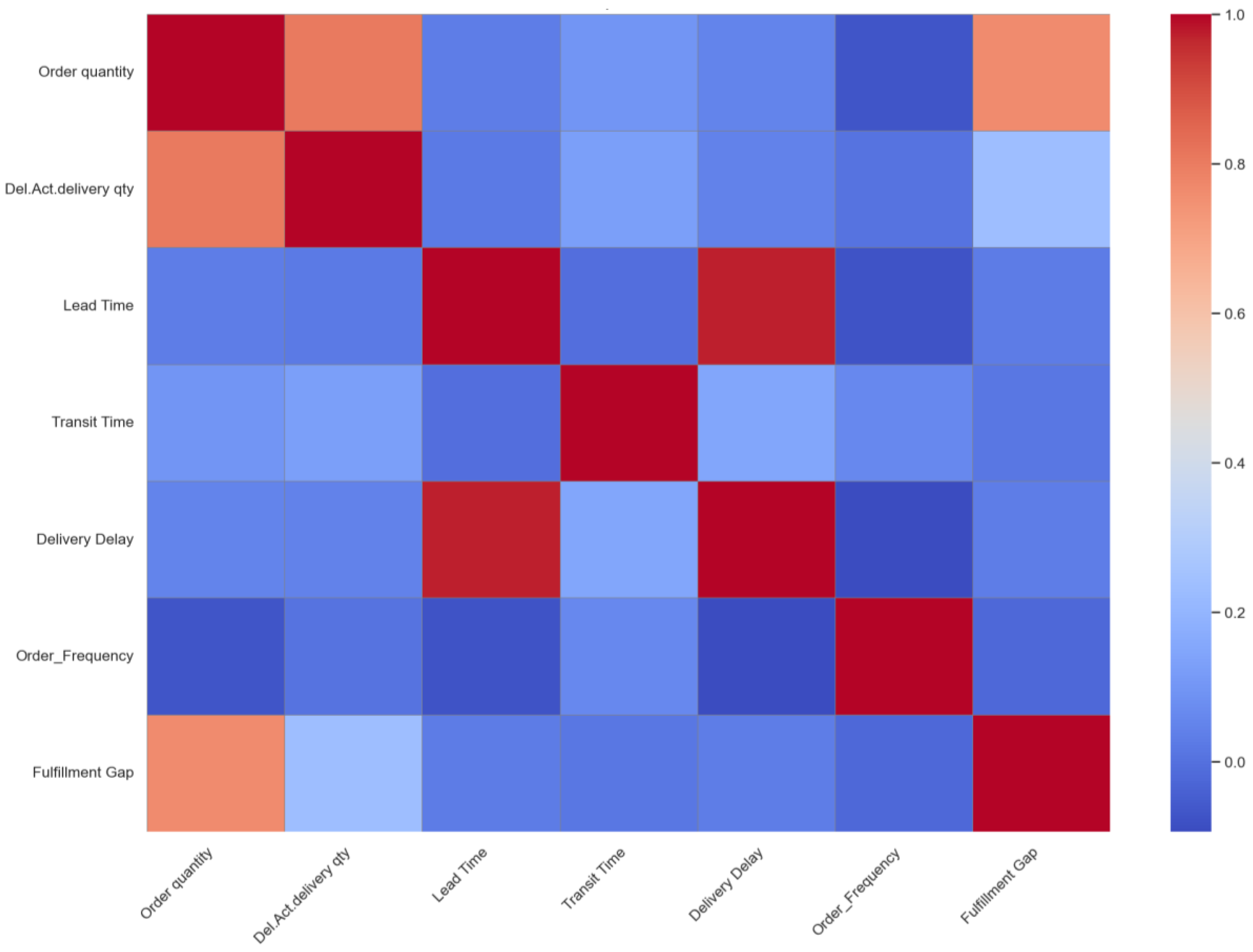
Figure 2.
Histogram Graph presenting the distribution of Delivery Delays.
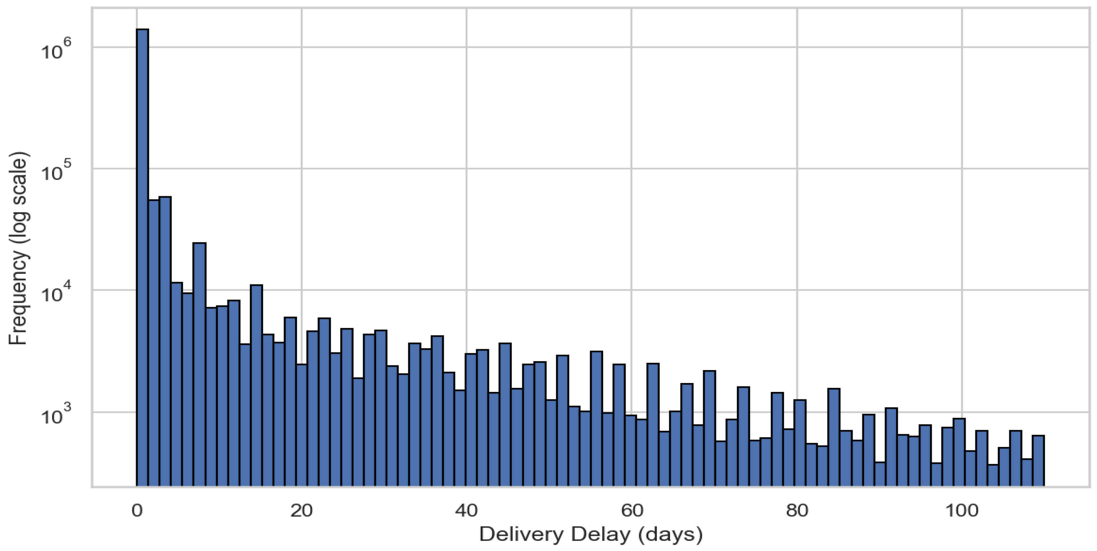
Figure 3.
Fulfillment Gap Histogram Graph (1% tails clipped).
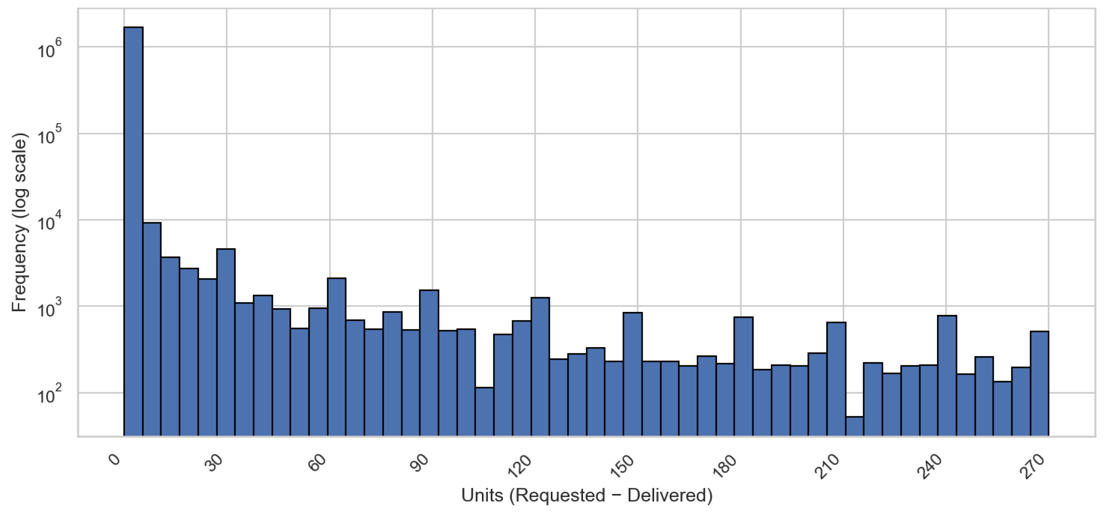
Figure 4.
Distribution Lead Time.
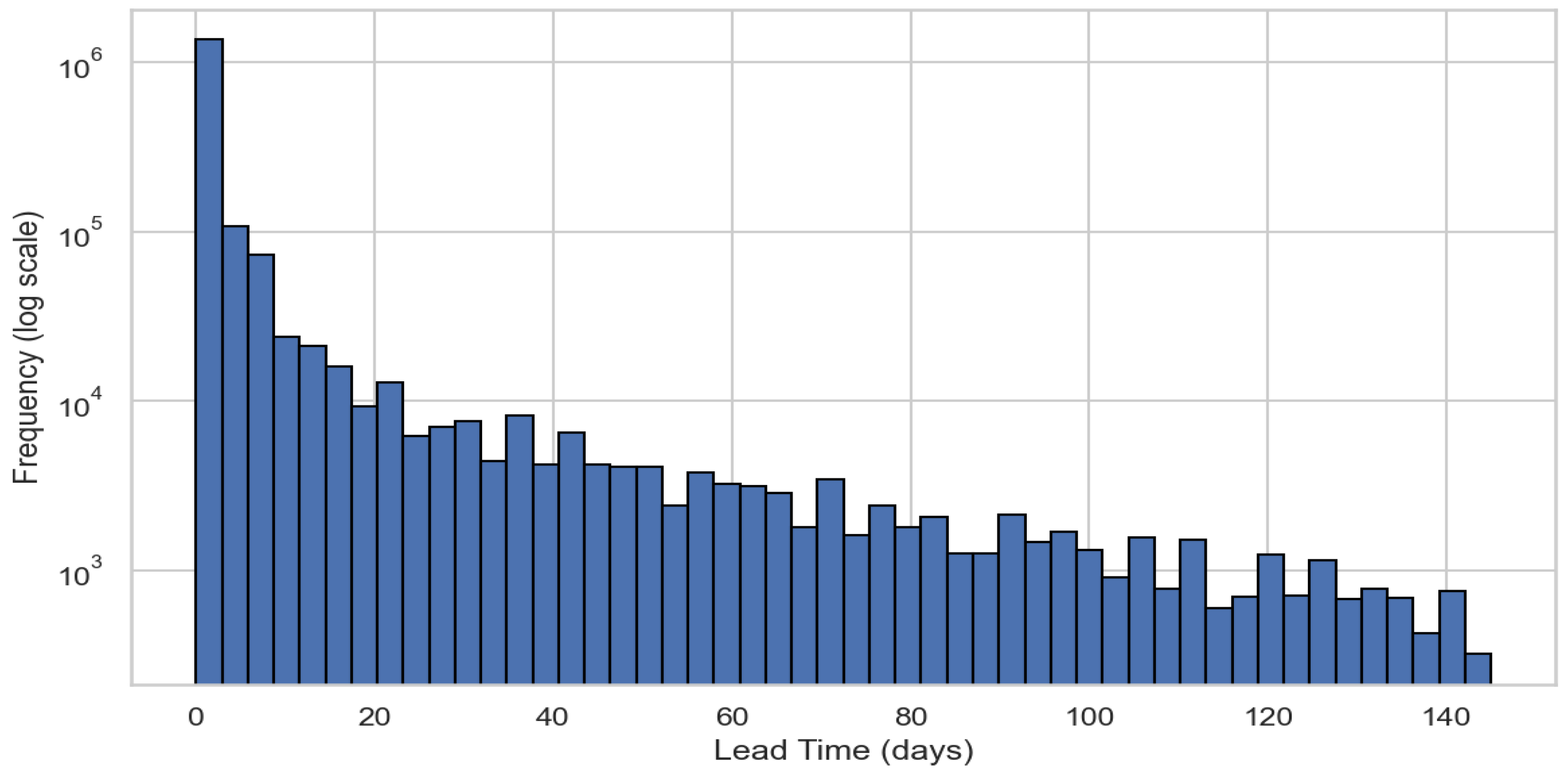
Figure 5.
Transit Time vs Delivery Delay.
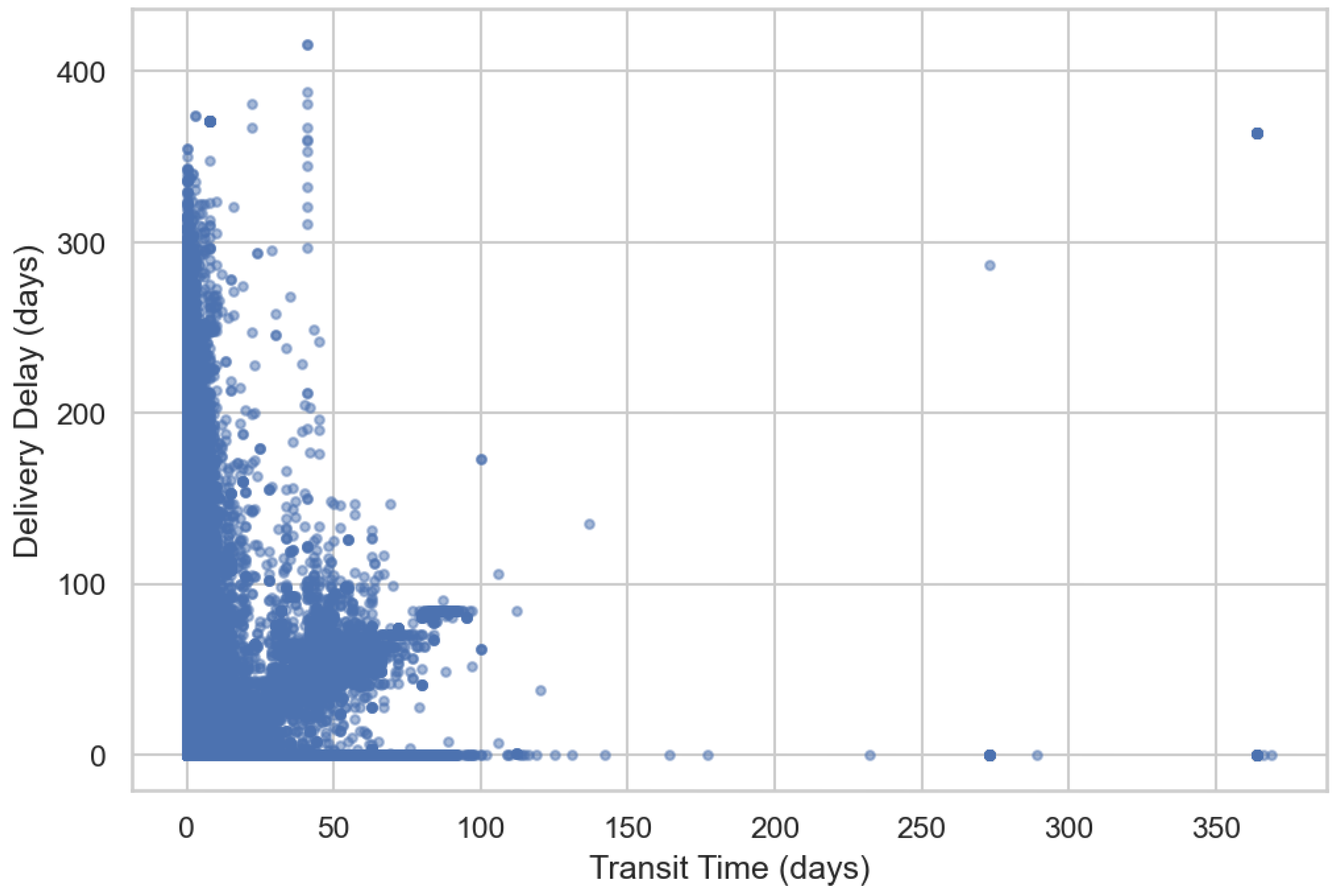
Figure 6.
Delivery Delay by Product Line.
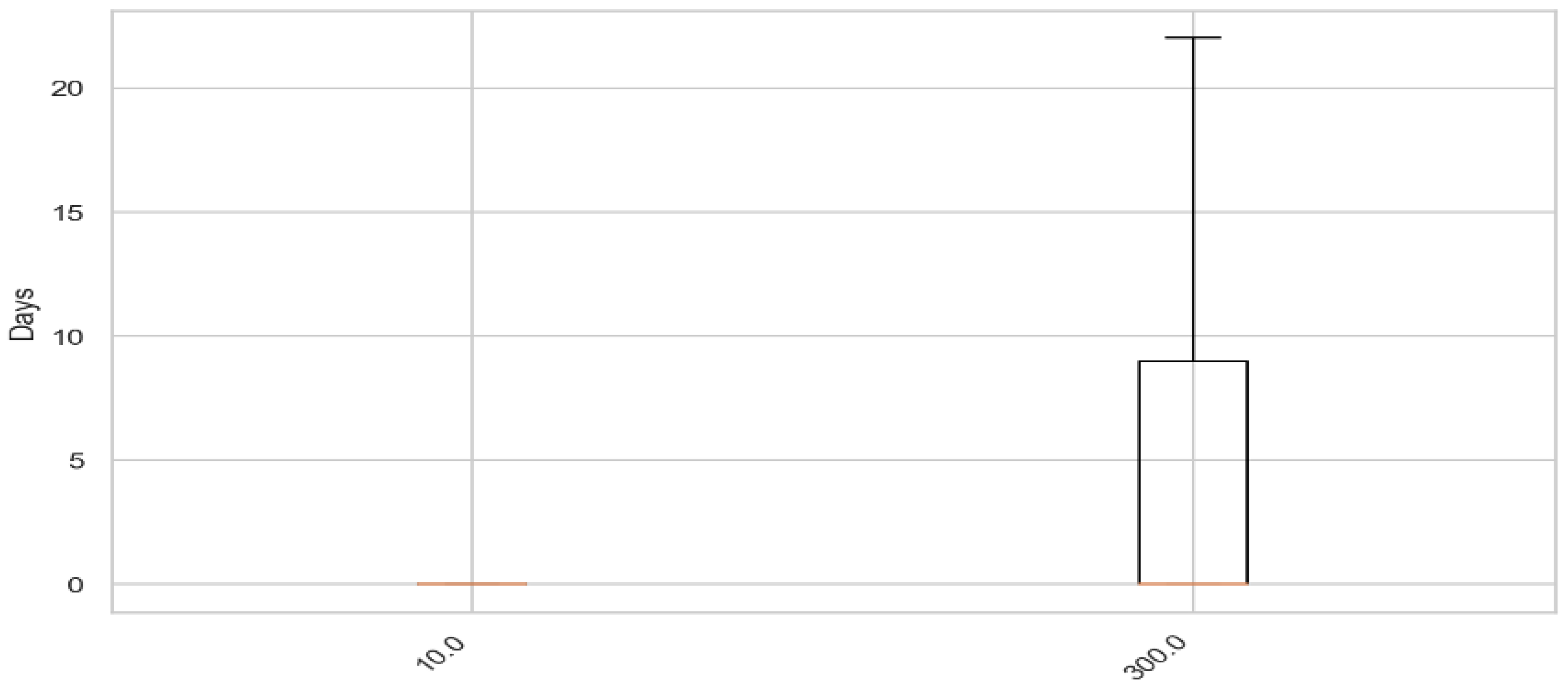
Figure 7.
On Time Performance (Monthly).
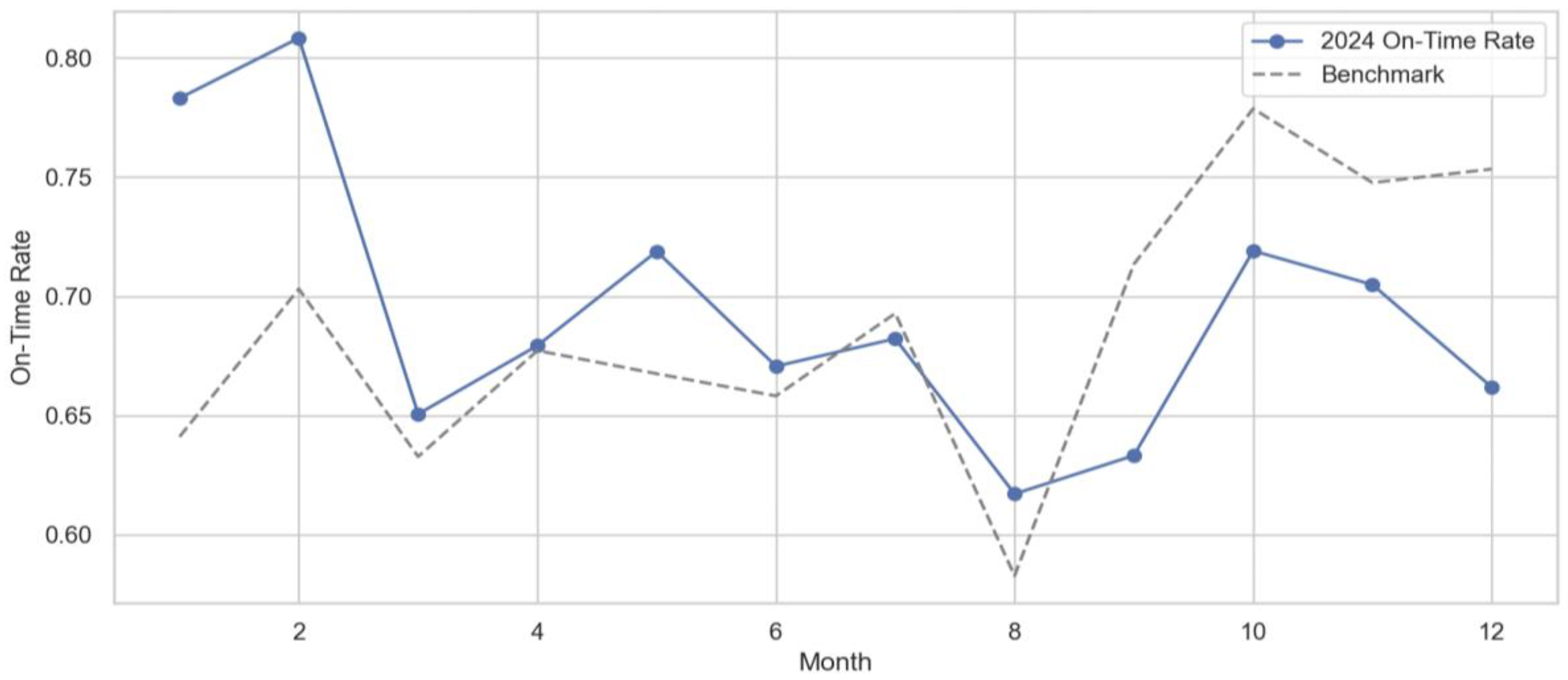
Figure 8.
Delivery Delay by Shipping Point.
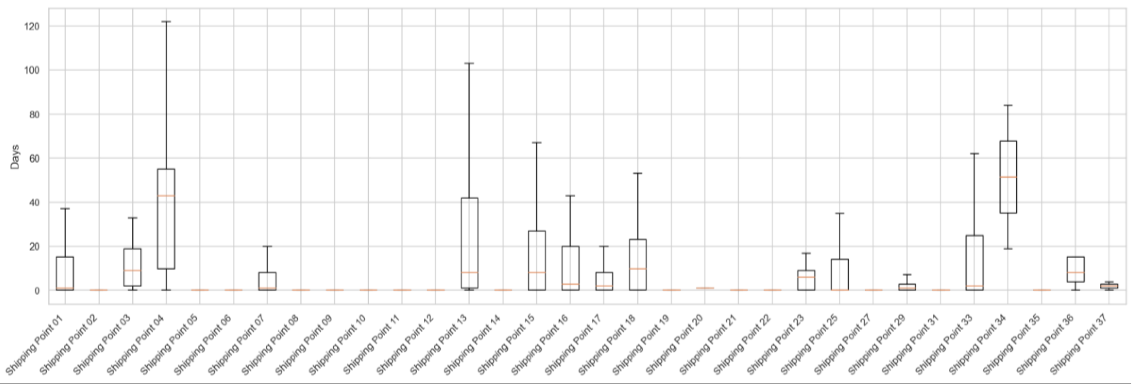
Figure 9.
Distribution of Delivery Delay (2024).
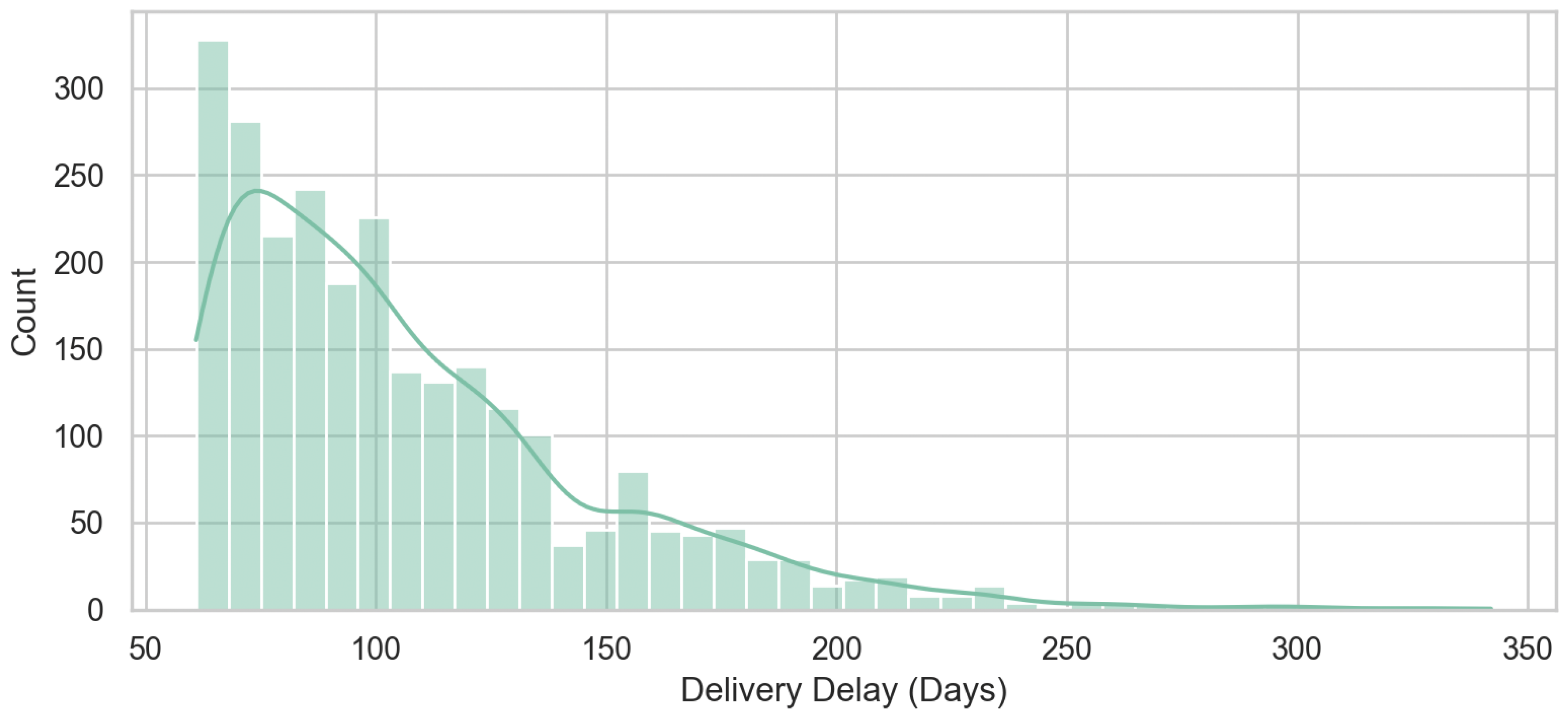
Figure 10.
Top 10 Anomalous Customers by Shipping Point.
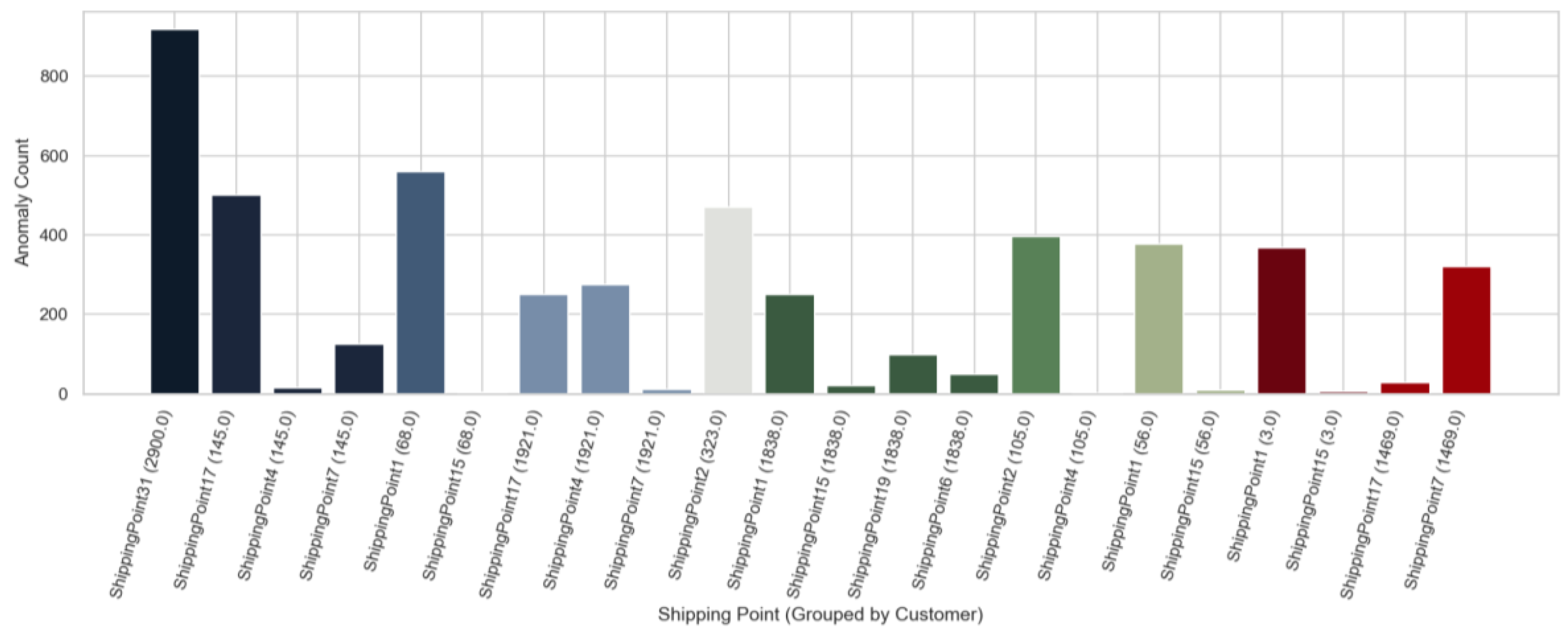
Figure 11.
Top 10 Anomalous Destination Countries.
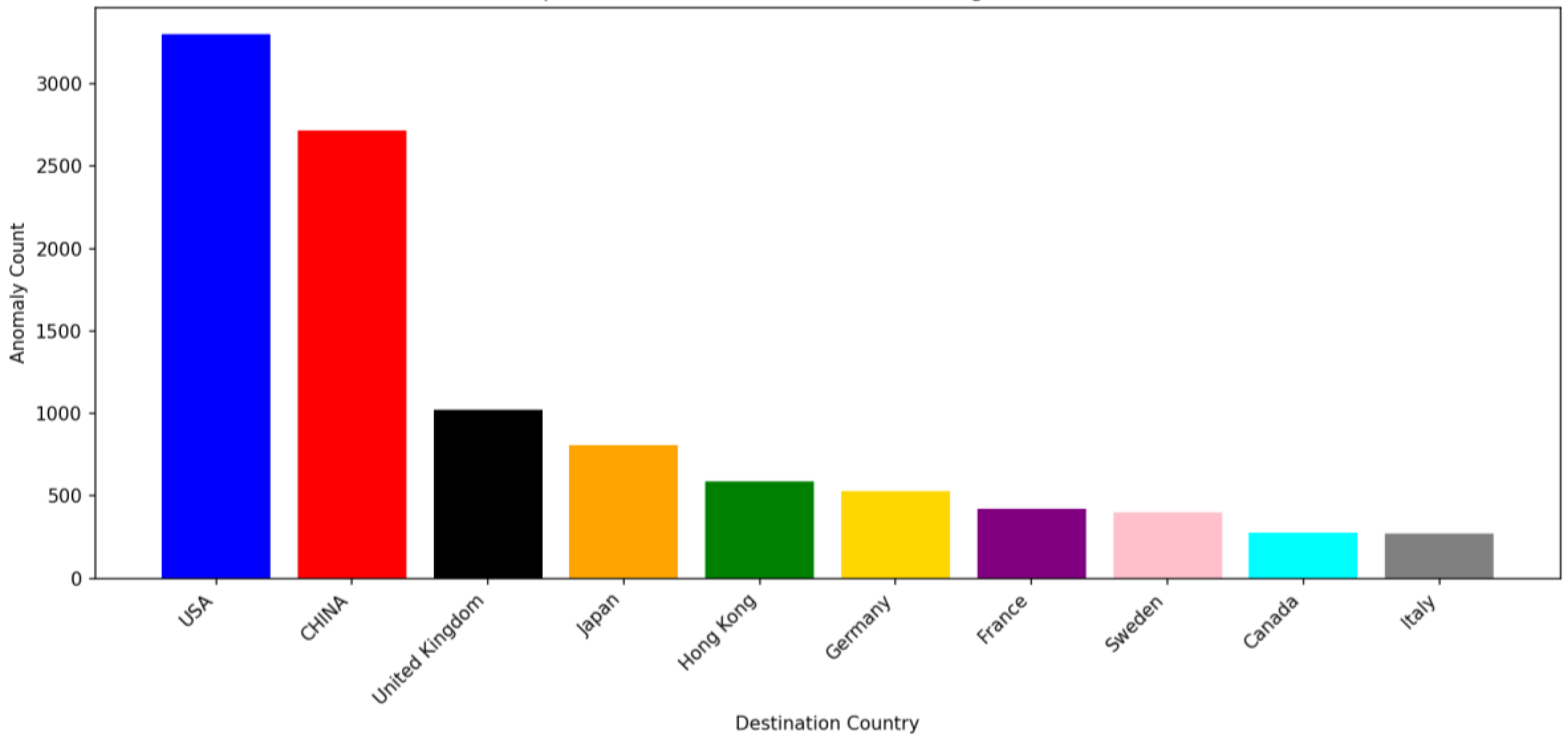
Figure 12.
Accuracy vs Contamination Rate.
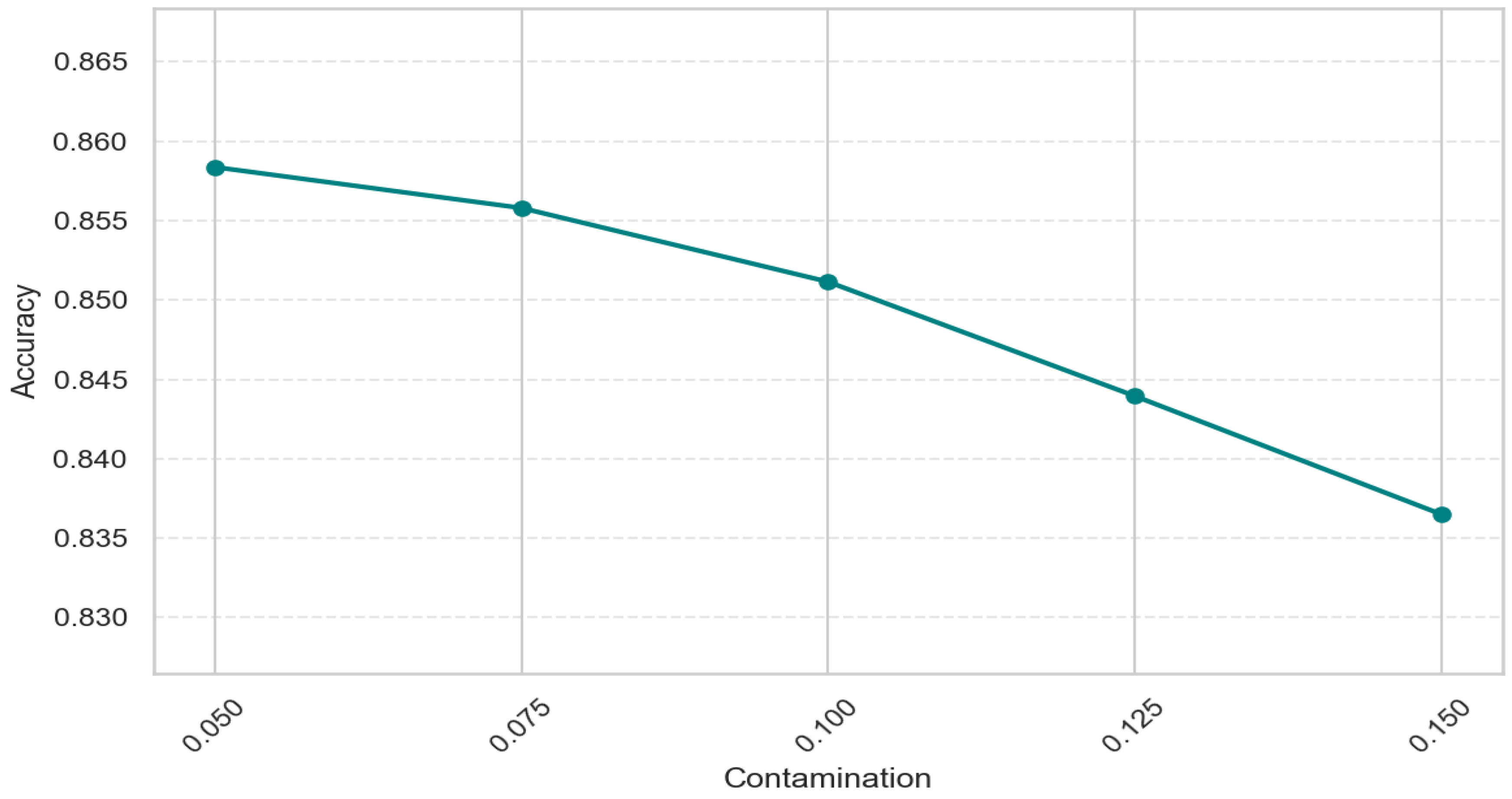
Figure 13.
Root Cause vs Percentage & Average Anomaly Score.
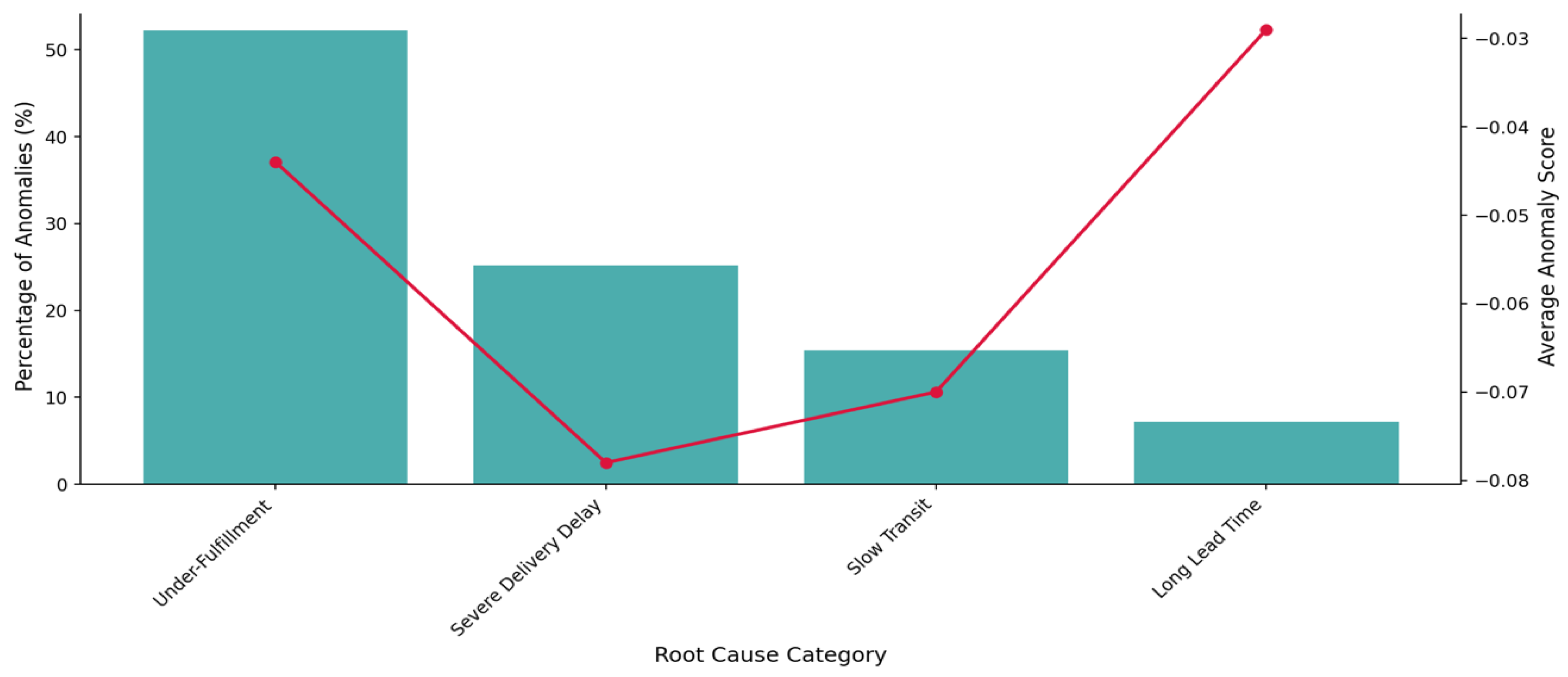
Figure 14.
Shipping Point Contributions to 2025 Anomalies.
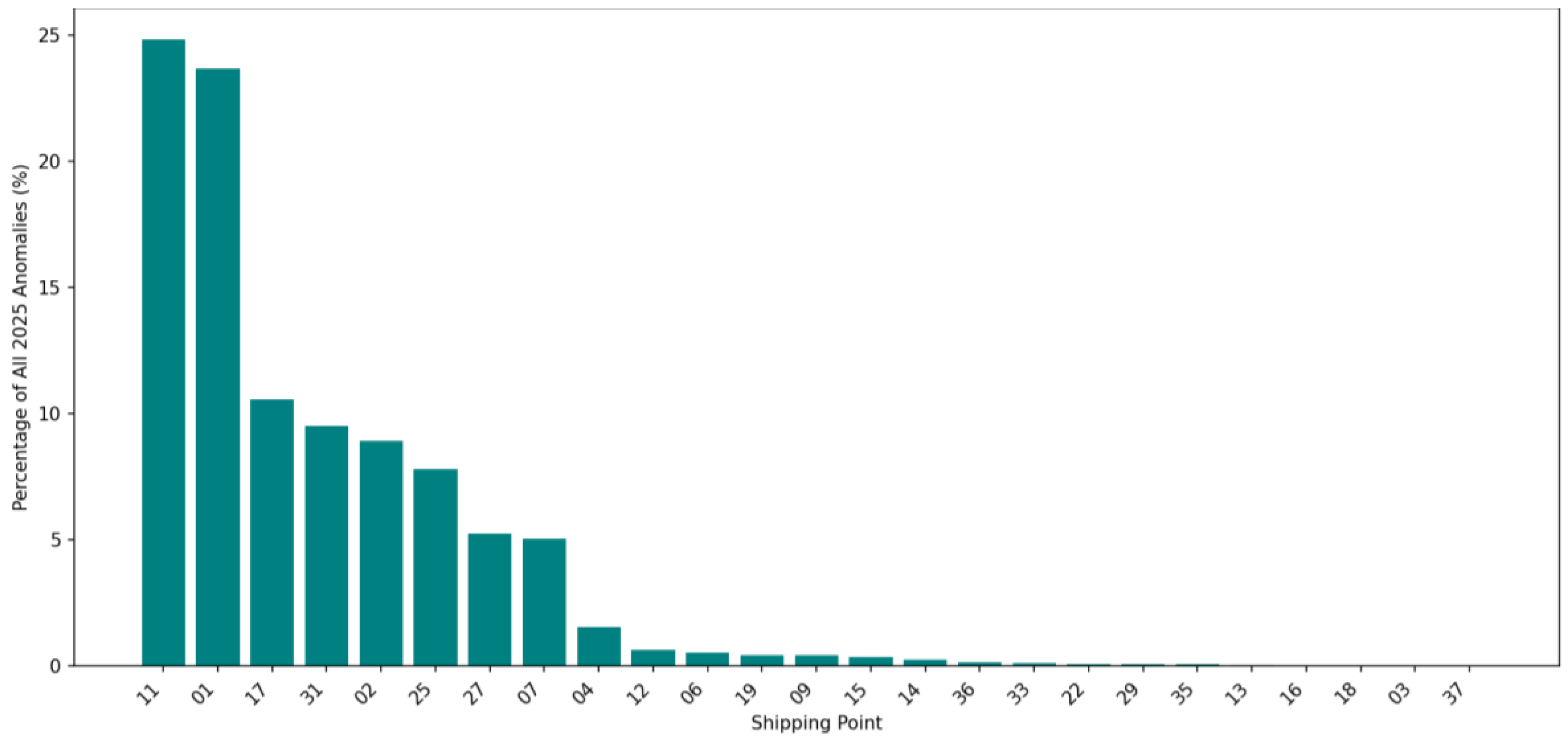
Figure 15.
2025 Predicted Anomalous Destination Country.
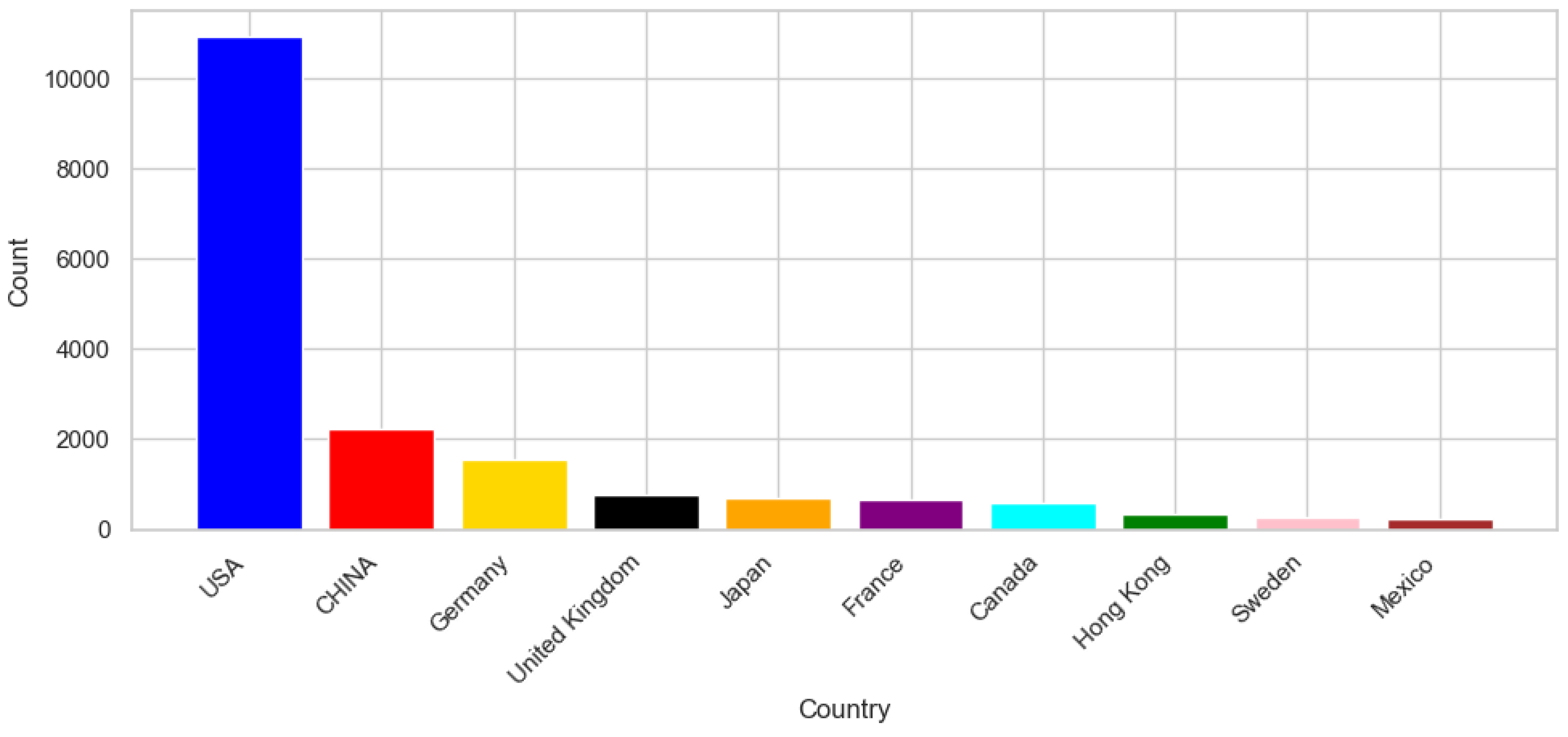
Figure 16.
Top 1,000 Anomalies Root Cause (%).
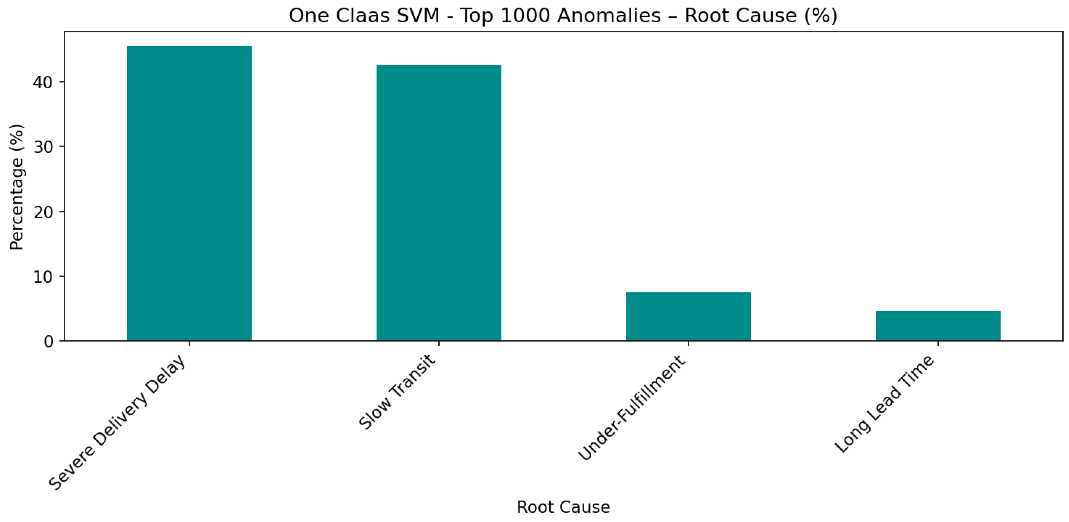
Figure 17.
Shipping Point Contribution to Anomalies.
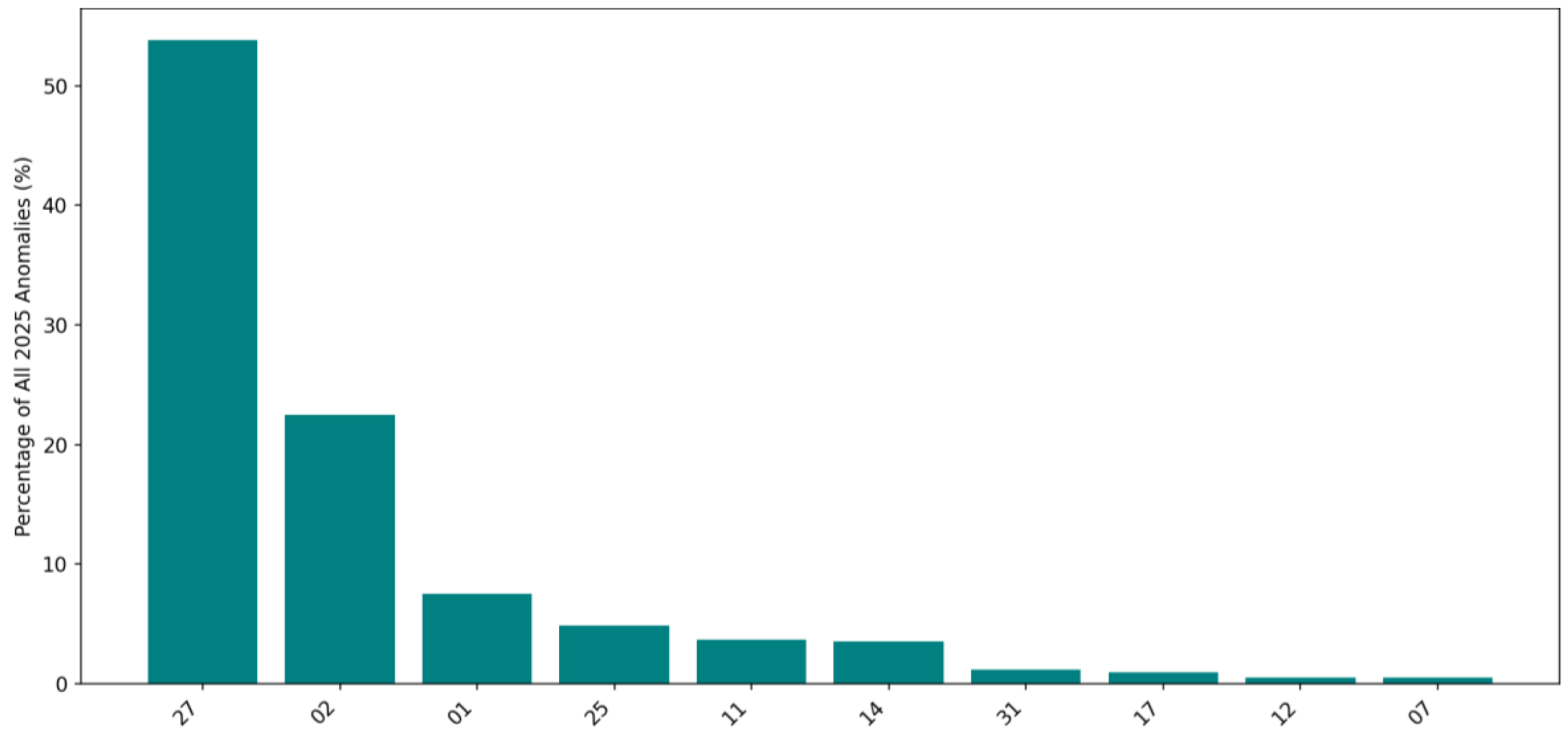

Table 1.
Steps and procedures for implementing the project.
| Step | Steps in This Research | Description |
|---|---|---|
|
Identify operational anomalies that contribute to shipment delays and partial fulfillment within B2B logistics. | Established the business problem and explained how anomaly detection supported improved delivery performance. |
|
Data Sources & Integration | Outlined the data structure and how it was prepared for analysis. |
| Scope Selection (2024) | Although EDA used 2020–2025 data to understand long-term patterns, model training was intentionally restricted to 2024, and 2025 data for testing. | |
| Metadata & Variable Definition | Defined variables and their roles used in EDA and model training. | |
| Exploratory Data Analysis | Examined variable distributions, correlations, and data patterns using visualizations. | |
|
Cleaning & Processing | Conducted data quality check and made sure the data is clean. |
| Feature Engineering | Created derived variables. | |
|
Model Development | Trained Isolation Forest and One Class SVM models |
|
Evaluate Results | Compared and visualized model results. |
|
Root Cause and business interpretation | Analyzed anomaly trends to uncover potential process inefficiencies and improvement opportunities. |
Table 2.
Features introduced to the models.
| Variable Name | Description | Type | Unit | Role in Analysis |
|---|---|---|---|---|
| Distribution Channel | Sales Distribution Channel representing various channels of movement (wholesale, distributor, direct, etc.) | Categorical | Code | Used to detect channel-specific delivery behavior patterns. |
| Number of units requested in the sales document order line. | Number of units requested in the sales document order line. | Numerical | Float | Core predictor of shipment complexity and processing load. |
| Del.Net Shipments | Net quantity shipped according to the delivery record. | Numerical | Units | Helps detect under-shipments and partial fulfillment behavior. |
| SoldTo | Customer identifier used for grouping deliveries. | Categorical Identifier | Integer | Captures customer-specific ordering behavior and recurring anomaly patterns. |
| Source_Sheet | Indicates the source dataset or batch from which the record originated. | Categorical | Text | Tracks data origin to ensure consistency across merged datasets. |
| Lead Time* | Number of days between Requested Ship Date and actual goods issue date. | Numerical | Days | Predictor capturing early-process delay dynamics before shipment. |
| Transit Time* | Number of days between actual goods issue date and actual delivery. | Numerical | Days | Predictor reflecting transportation efficiency and logistics delays. |
| Order_Frequency* | Count of sales orders placed by a customer in a given month, based on the Sales Document Creation Date. | Numerical | Integer | Behavioral predictor capturing demand intensity and ordering patterns. |
| Fulfillment Gap* | Difference between Requested Quantity and Delivered Quantity. | Numerical | Integer | Identifies shortages and partial deliveries contributing to delays. |
Note. * Derived Variables.
Table 3.
Descriptive Statistics (2020 to 2025).
| Row Count | Mean | STD | MIN | MAX | |
|---|---|---|---|---|---|
| Delivery Delay | 1,745,869 | 6.0 | 20.0 | 0.0 | 416.0 |
| Transit Time | 4,710,125 | 2.0 | 7.0 | 0.0 | 369.0 |
| Lead Time | 1,746,055 | 6.5 | 20.0 | 0.0 | 375.0 |
Table 4.
Isolation Forest Anomaly Score Summary.
| Count | Mean | STD | Min | 25% | 50% | 75% | Max |
|---|---|---|---|---|---|---|---|
| 15,501 | -0.07 | 0.06 | -0.27 | -0.10 | -0.05 | -0.02 | 0 |
Table 5.
Top 10 Anomalous Shipping Points.
| Shipping Point | Anomaly Concentration % |
|---|---|
| ShippingPoint1 | 23.2 |
| ShippingPoint25 | 16.3 |
| ShippingPoint17 | 16.0 |
| ShippingPoint7 | 12.1 |
| ShippingPoint31 | 9.9 |
| ShippingPoint2 | 8.8 |
| ShippingPoint27 | 4.6 |
| ShippingPoint4 | 4.0 |
| ShippingPoint12 | 1.1 |
| ShippingPoint19 | 1.0 |
| ShippingPoint15 | 0.6 |
| Other | 2.4 |
Table 6.
Confusion Matrix 2024 Data.
| Predicted Normal | Predicated Anomaly | |
|---|---|---|
| Actual Normal | 279,014 (TN) | 7,379 (FP) |
| Actual Anomaly | 15,498 (FN) | 8,122 (TP) |
Table 7.
Confusion Matrix 2025 Data.
| Predicted Normal | Predicated Anomaly | |
|---|---|---|
| Actual Normal | 235,799 (TN) | 10,803 (FP) |
| Actual Anomaly | 29,145 (FN) | 9,683 (TP) |
Table 8.
Shipping Point Anomalous Percentage 2024-2025.
| Shipping Point | 2024 Anomaly Concentration % | 2025 Anomaly Concentration % |
|---|---|---|
| ShippingPoint11 | 0.4 | 24.8 |
| ShippingPoint1 | 23.2 | 24.1 |
| ShippingPoint17 | 16.0 | 11.0 |
| ShippingPoint31 | 9.9 | 9.5 |
| ShippingPoint2 | 8.8 | 8.9 |
| ShippingPoint25 | 16.3 | 8.0 |
| ShippingPoint27 | 4.6 | 5.2 |
| ShippingPoint7 | 12.1 | 5.0 |
| ShippingPoint27 | 4.6 | 5.2 |
| ShippingPoint4 | 4.0 | 1.5 |
| ShippingPoint12 | 1.1 | 0.6 |
| ShippingPoint19 | 1.0 | 0.4 |
| ShippingPoint15 | 0.6 | 0.4 |
| Other | 2.0 | 0.6 |
Table 9.
Comparison of Shipping Point Anomalies.
| Shipping Point | Percentage Isolation Forest% | Percentage One Class SVM% |
|---|---|---|
| ShippingPoint11 | 25 | 4 |
| ShippingPoint17 | 11 | 1 |
| ShippingPoint1 | 24 | 8 |
| ShippingPoint25 | 8 | 5 |
| ShippingPoint31 | 9 | 1 |
| ShippingPoint7 | 5 | 1 |
| ShippingPoint2 | 9 | 22 |
| ShippingPoint27 | 5 | 54 |
| ShippingPoint4 | 2 | 1 |
| ShippingPoint19 | 1 | 1 |
| ShippingPoint12 | 1 | 2 |
Disclaimer/Publisher’s Note: The statements, opinions and data contained in all publications are solely those of the individual author(s) and contributor(s) and not of MDPI and/or the editor(s). MDPI and/or the editor(s) disclaim responsibility for any injury to people or property resulting from any ideas, methods, instructions or products referred to in the content. |
© 2025 by the authors. Licensee MDPI, Basel, Switzerland. This article is an open access article distributed under the terms and conditions of the Creative Commons Attribution (CC BY) license (http://creativecommons.org/licenses/by/4.0/).
Copyright: This open access article is published under a Creative Commons CC BY 4.0 license, which permit the free download, distribution, and reuse, provided that the author and preprint are cited in any reuse.


