Quantifying the Relationship Between Blue-Green Landscape Spatial Patterns and Carbon Storage: A Case Study of Zhengzhou Metropolitan Area

1. Introduction

Human activities have exacerbated global warming (Cox, 2013). In response, both international and domestic measures have been implemented. Urban areas are a major factor contributing to climate change, as cities, occupying less than 2% of the Earth’s surface, consume 78% of the world’s energy and emit over 60% of greenhouse gases. As a result, cities and metropolitan areas are crucial carriers for achieving the “dual carbon” goals. BGS, consisting of green plant areas and blue water bodies, form an interconnected whole that not only serves as the foundation for urban ecological networks but also plays a significant role in enhancing urban resilience and reducing carbon emissions (Sanchez and Govindarajulu, 2023). They represent a complex and diverse ecosystem with multiple ecological benefits, such as stormwater management (Almaaitah, 2021), mitigating the urban heat island effect (Chen, 2022), and enhancing urban carbon sequestration (He, 2020). Green spaces include agricultural land, mountains, forests, grasslands, parks, and other vegetated areas, while blue spaces encompass rivers, lakes, reservoirs, ponds, beaches, and other water bodies (Huang, 2022). Landscape patterns generally refer to their spatial arrangements, reflecting the interactions among different landscape patches, corridors, and matrices. These patterns not only embody the heterogeneity of landscapes but also represent the results of various ecological processes at different scales. In the context of the “dual carbon” goals, urban BGS are important means for carbon reduction. Research suggests that green spaces are primary carriers of carbon sequestration, capable of absorbing one-quarter of urban carbon dioxide emissions annually (Zhao, 2021). Simultaneously, BGS serves as significant carbon sinks, absorbing and storing carbon.

Carbon storage (CS) mainly includes aboveground biomass CS, belowground biomass CS, soil organic CS, and dead organic matter CS (Sun and Liu, 2019). These are important indicators of urban ecosystem service functions. Accurately estimating CS within a region and exploring its spatial distribution patterns and influencing factors is crucial for enhancing and managing the carbon sink function of urban ecosystems. Traditional methods for estimating CS, such as soil type analysis, life zones, plot surveys, and biomass measurements, are relatively accurate and widely used (Zhang, 2022). However, these methods are resource-intensive, requiring substantial human effort, materials, and time. Additionally, they are not well-suited for studying long-term, large-scale changes in CS and their influencing mechanisms. Model-based CS estimation methods can effectively address the shortcomings of traditional methods. These methods offer advantages such as ease of operation, wide applicability, extensive information, and cost-effectiveness (Wang, 2022), making them suitable for large-scale CS estimation. They can be divided into process-based and non-process-based modeling methods. Process-based modeling methods excel in simulating small areas but require numerous parameters, limiting their applicability in larger regions (Lemma, 2021). In contrast, non-process-based modeling methods require fewer parameters and are thus more suitable for large-scale studies (Zhang, 2022). The InVEST (Integrated Valuation of Ecosystem Services and Trade-offs) model is one of the most widely used non-process-based models, primarily driven by land use data. It can effectively assess CS across various ecosystem types based on large-scale land use changes (Bera, 2022).

In the overall strategy for achieving carbon neutrality, many countries are enhancing their efforts to reduce and store carbon in urban areas. Adjusting the morphological structure and layout of BGS has become an important means of reducing carbon emissions and increasing CS in the era of stock. Northwest proposed a method using the Fragstats program to quantify landscape patterns of environmental components (Mcgarigal and Marks, 1995). This method has been widely applied to assess the impacts of BGS on climate change and other factors. Rejaur found that the high fragmentation and reduced connectivity of BGS increase urban vulnerability to climate change impacts (Ran, 2023). Han (2018) studied morphological changes in green spaces in South Korea and their effects on CS, revealing that the reduction of green space area and patch fragmentation are associated with decreased carbon sequestration. Yuan et al. (2023) demonstrated that increasing the area and connectivity of BGS benefits carbon sink capacity, while separation and shape indices negatively impact this capacity. By quantifying various landscape indices of different types of BGS, they provided a basis for optimizing BGS systems. For example, a study by Zhang (2024) highlighted the spatiotemporal impacts of BGS on carbon emissions in China’s Yangtze River Delta. However, existing studies mainly focus on the relationship between green spaces and carbon sinks, with limited research on the inter-regional correlations of BGS morphology and layout with CS, especially considering their spatial heterogeneity. Traditional regression analysis methods have been widely used to explore the relationship between BGS and CS. However, these methods assume a uniform relationship among all observation points, overlooking heterogeneity in geographical space, which may lead to inaccuracies and limitations in interpretation of results. To overcome this limitation, spatial statistical methods such as Geographic Weighted Regression (GWR) and multiscale geographically weighted regression (MGWR) have been developed. GWR introduces a spatial weight matrix to conduct regression analysis at each geographical location, capturing the local relationships between variables (Wu et al., 2024). This approach enables researchers to reveal regional differences in the impact of BGSPs on carbon sinks. However, GWR is limited by its reliance on a single spatial scale for analysis. MGWR addresses this limitation by assigning different spatial scales to different explanatory variables, allowing for a more precise capture of the complex spatial relationships and enhancing the accuracy and interpretability. This method is commonly used to address the spatial influence of factors (Zhao et al., 2024). Therefore, this study utilized the InVEST model to estimate CS within the research area and quantified the landscape patterns of urban BGS. We further analyzed the spatial heterogeneity of the effects of different explanatory variables at different spatial scales using both GWR and MGWR. With the aim of optimizing urban BGS to CS storage in urban ecosystems, the specific research objectives are: (1) to quantify the correlation between the overall and internal landscape patterns of BGS and CS in the Zhengzhou Metropolitan Area, along with key indicators; (2) to analyze the spatial heterogeneity of the impacts of different explanatory variables at different spatial scales using MGWR and other methods; (3) to propose planning methods aimed at enhancing CS through improved urban BGS, providing references for urban planning and resource management practices.

2. Materials and Methods

2.1. Study Area

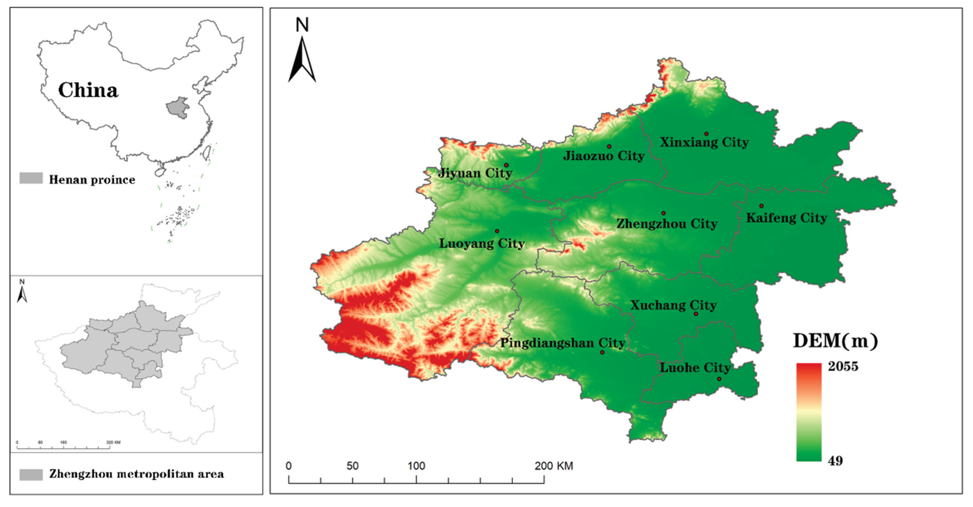
The Zhengzhou Metropolitan Area, located in central China in the middle and lower reaches of the Yellow River, is an urban functional region composed of closely connected cities such as Zhengzhou, Kaifeng, Xuchang, Xinxiang, Jiaozuo, Luoyang, Pingdingshan, and Luohe. In June 2024, the Zhengzhou Metropolitan Area Development Plan was officially released. As the tenth national-level metropolitan area in China, Zhengzhou features a predominantly plain topography. The varying levels of development among cities within the Zhengzhou Metropolitan Area have led to distinct landscape patterns. As the core of Henan Province, the relationship between CS and the landscape patterns of urban BGS in the Zhengzhou metropolitan area is of significant importance for achieving the “dual carbon” goals.

Figure 1. Location of the study area (NO. GS (2022) 4308).

Figure 1. Location of the study area (NO. GS (2022) 4308).

2.2. Data Sources

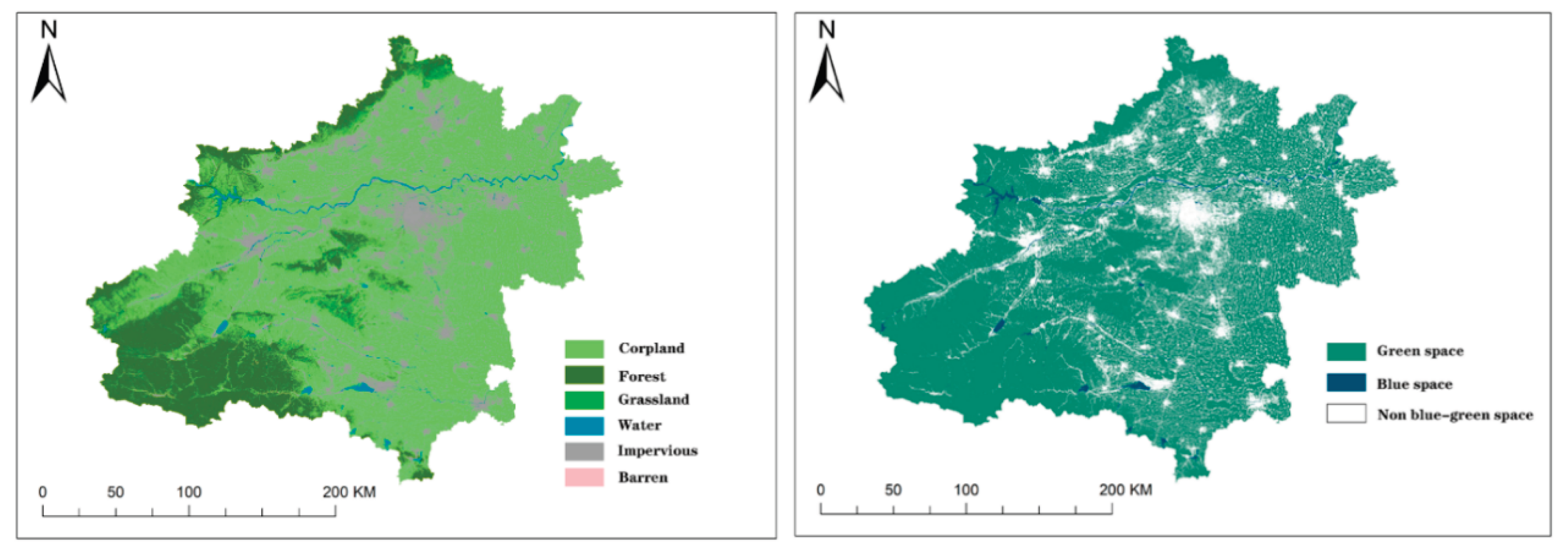
The 30-meter spatial resolution land use data for the Zhengzhou Metropolitan Area in 2022 was obtained from the Resource and Environment Science and Data Center of the Chinese Academy of Sciences (CAS). Based on the definition and classification of BGS (Zhao et al., 2024), the ArcMap reclassification tool in ArcGIS 10.8 was used to classify arable land, forest land, and grassland as green spaces, water bodies as blue spaces, and construction land and unused land as non-BGSs. This resulted in a distribution map of urban BGS, which served as the foundational dataset for further BGSP analysis.

Figure 2. Land use data of cities of Zhengzhou Metropolitan Area in 2022 (NO. GS (2022) 4308).

Figure 2. Land use data of cities of Zhengzhou Metropolitan Area in 2022 (NO. GS (2022) 4308).

Carbon density data are a crucial input for the InVEST model. In this study, a carbon density correction method was used to determine the carbon density of the study area. First, comprehensive carbon density data for the entire country were obtained by referencing relevant studies (Fanghu et al., 2023; Li et al., 2003; Alam et al., 2013; Giardina et al., 2000; Guangshui et al., 2007).

Table 1. Carbon density of various parts of different land-use types in China (t·hm^-2).

Land Use Type	Aboveground Carbon Storage	Belowground Carbon Storage	Soil Organic Carbon Storage
Cropland	5.7	80.7	108.4
Forest	42.4	115.9	158.8
Grassland	35.3	86.5	99.9
Water	3	0	0
construction land	2.5	0	78
unused land	1.3	0	31.4

Table 1. Carbon density of various parts of different land-use types in China (t·hm^-2).

Land Use Type	Aboveground Carbon Storage	Belowground Carbon Storage	Soil Organic Carbon Storage
Cropland	5.7	80.7	108.4
Forest	42.4	115.9	158.8
Grassland	35.3	86.5	99.9
Water	3	0	0
construction land	2.5	0	78
unused land	1.3	0	31.4

The national and Henan Province average temperature and precipitation data used in this study were sourced from the National Meteorological Information Center—China Meteorological Data Service Center (https://data.cma.cn/).

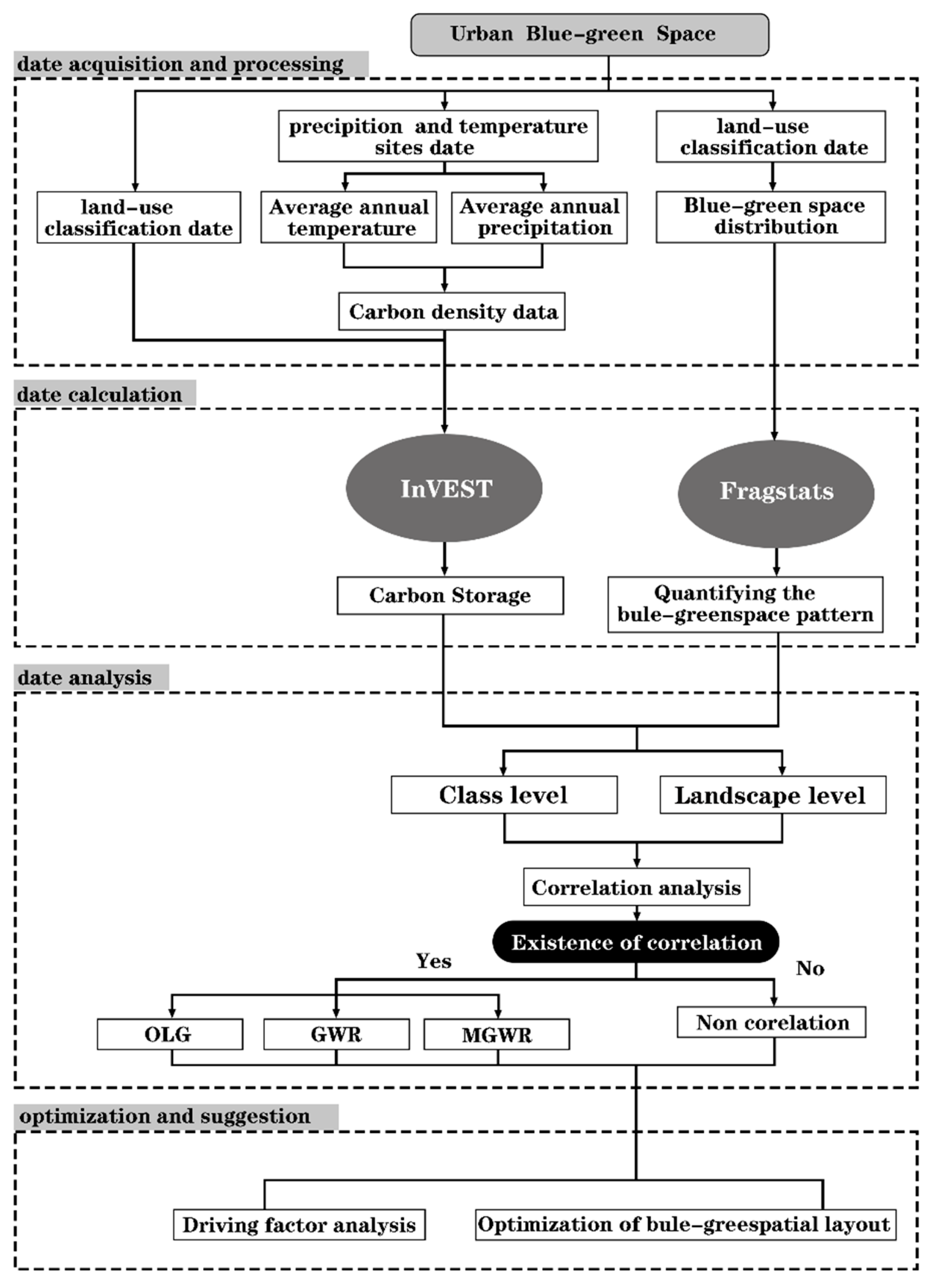
2.3. Data Analysis Procedures

This study comprised four main steps: data collection and processing, data calculation, data analysis, and optimization recommendations, as illustrated in the following flowchart.

Figure 3. Methodology flowchart of the study.

Figure 3. Methodology flowchart of the study.

2.4. CS Calculation in the Study Area

In this study, the CS within the study area was estimated using the carbon module of the InVEST model. The total CS was divided into four basic carbon pools: aboveground biomass carbon pool, belowground biomass carbon pool, soil organic carbon pool, and dead organic matter carbon pool. The formula is as follows:

$$C_{\mathrm{t}\mathrm{o}\mathrm{t}\mathrm{a}\mathrm{l}i}=\sum _{j=1}^n{A}_{ij}\times \left(C_{aj}+C_{bj}+C_{cj}+C_{dj}\right)$$

(1)

where $C_{\mathrm{t}\mathrm{o}\mathrm{t}\mathrm{a}\mathrm{l}i}$ represents the total CS (t); $A_{ij}$ is the area of each land use type j (hm²); $C_{aj}$, $C_{bj}$, $C_{cj}$, and $C_{dj}$ are the aboveground biomass carbon density, belowground biomass carbon density, soil carbon density, and dead organic matter carbon density (t·hm²) corresponding to each land use type j; n is the number of land use types.

2.5. Carbon Density Correction

Carbon density, defined as the CS per unit of land use area, is a crucial input parameter in the CS calculation of the InVEST model. Carbon density varies with changes in climate, soil properties, and land use types. Regional differences in these factors can significantly affect the final CS calculation, necessitating a correction. Both aboveground and belowground carbon densities are positively correlated with annual precipitation and average annual temperature, while soil carbon density is positively correlated with annual precipitation. The carbon density for various land use types in the Zhengzhou Metropolitan Area was corrected using the methods proposed by Alam32, Giardina38, and Chen Guangshui39, as shown in equations (2), (3), and (4).

$$C_{SP}=3.3968\times P+3996.1 \left(R^2=0.11\right)$$

(2)

$$C_{BP}=6.798e^{0.0054P}\left(R^2=0.70\right)$$

(3)

$$C_{BT}=28\times T+398 \left(R^2=0.47,P<0.01\right)$$

(4)

where $C_{SP}$ represents the soil carbon density (t·hm²) calculated based on the average annual precipitation; $C_{BP}$ and $C_{BT}$ represent the biomass carbon densities (t·hm²) calculated based on the average annual precipitation and average annual temperature; $P$ is the average annual precipitation (mm); $T$ is the average annual temperature (°C).

By substituting the average annual precipitation and temperature values for Henan Province and China into the above formulas (where the average annual temperature in Henan Province in 2022 was 15.8°C, and the average annual precipitation was 621.7 mm; the average annual temperature in China in 2022 was 10.5°C, and the average annual precipitation was 606.1 mm), the correction coefficient can be obtained. The carbon density data for Henan Province is then calculated by multiplying the national carbon density data by the correction coefficient. The specific formula is as follows:

$$K_{BP}={\displaystyle \frac{C_{BP}^{\prime }}{C_{BP}^{″}}}$$

(5)

$$K_{BT}={\displaystyle \frac{C_{BT}^{\prime }}{C_{BT}^{″}}}$$

(6)

$$K_B={\displaystyle \frac{K_{BP}}{K_{BT}}}$$

(7)

$$K_S={\displaystyle \frac{C_{SP}^{\prime }}{C_{SP}^{″}}}$$

(8)

where $K_B$ and $K_S$are the soil carbon density correction coefficient and biomass carbon density correction coefficient for Henan Province, respectively.$K_{BP}$ and $K_{BT}$ are the correction coefficients for the precipitation and temperature factors affecting biomass carbon density. $C_{BP}^{\prime }$ is the biomass carbon density value for Henan Province calculated based on average annual precipitation.$C_{BT}^{\prime }$ is the biomass carbon density value for Henan Province calculated based on average annual temperature.$C_{SP}^{\prime }$ is the soil carbon density value for Henan Province calculated based on average annual precipitation.$C_{BP}^{\prime \prime }$ is the biomass carbon density value for China calculated based on average annual precipitation.${ C}_{BT}^{\prime \prime }$ is the biomass carbon density value for China calculated based on average annual temperature.${ C}_{SP}^{\prime \prime }$ is the soil carbon density value for China calculated based on average annual precipitation. After calculating the carbon density correction coefficients and applying them to the national carbon density values, the carbon density values for Henan Province are obtained.

Table 2. Revised carbon intensity parameter of Henan Province(t·hm⁻²).

	Land Use Type	Aboveground Carbon Storage	Belowground Carbon Storage	Soil Organic Carbon Storage
1	Cropland	5.75	81.41	111.23
2	Forest	42.77	116.91	116.47
3	Grassland	35.61	87.26	101.58
4	Water	3.03	0	0
5	Construction land	2.52	0	79.31
6	Unused land	1.31	0	31.93

Table 2. Revised carbon intensity parameter of Henan Province(t·hm⁻²).

	Land Use Type	Aboveground Carbon Storage	Belowground Carbon Storage	Soil Organic Carbon Storage
1	Cropland	5.75	81.41	111.23
2	Forest	42.77	116.91	116.47
3	Grassland	35.61	87.26	101.58
4	Water	3.03	0	0
5	Construction land	2.52	0	79.31
6	Unused land	1.31	0	31.93

2.6. Quantification of BGSPs

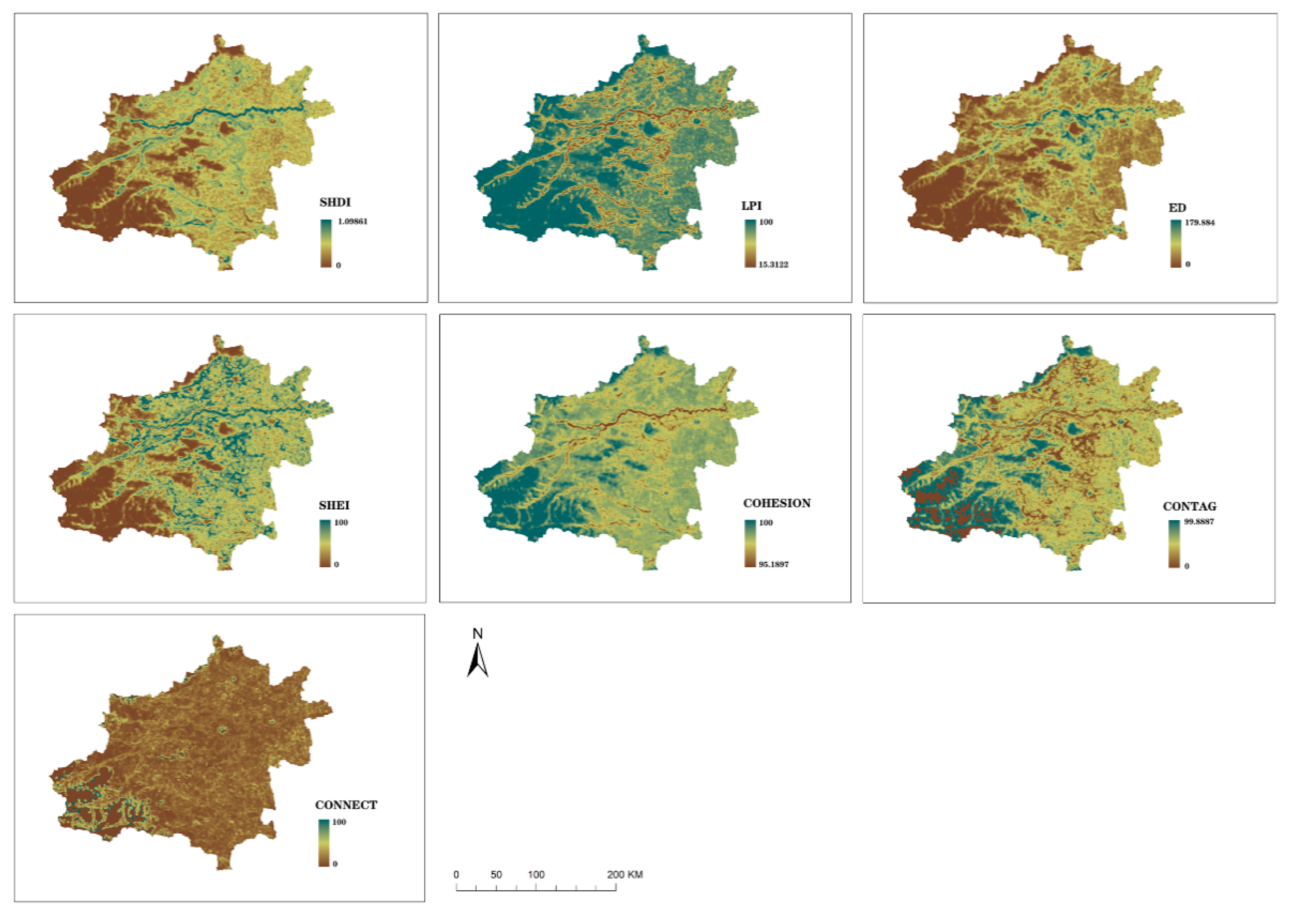
The landscape pattern of the blue-green system refers to the spatial configuration of urban blue spaces, green spaces, and non-BGSs at various scales. Landscape scales are quantitative indicators reflecting the characteristics of the urban blue-green system and can be divided into three levels: patch level, class level, and landscape level (Wu, 2000). Patch Level primarily reflects the characteristics of individual patches, forming the basis for calculating other landscape-level indicators and focusing on the specific attributes and morphology of individual patches. Class Level reflects the structural characteristics of different patch types, examining the distribution and attributes of various patch types within the landscape, analyzing their interactions and relationships, as well as their contributions to the overall functionality of the landscape. Landscape Level reflects the overall structural characteristics of the landscape, focusing on the composition, spatial configuration, and dynamic changes of the entire landscape system. It is used to assess the heterogeneity, diversity, fragmentation degree, and spatial relationships between landscape elements, which are crucial for understanding the ecological processes and functions of the landscape (Chen et al., 2002). In this study, the moving window method was used to assess landscape pattern indicators, allowing for the characterization of spatial dynamic changes in these indicators. This method considers scale effects (Yuan et al., 2023). The internal and overall patterns of BGS are quantified separately at the class level and landscape level. The selected indicators are categorized into five types: area-edge, shape complexity, aggregation, connectivity, and diversity (Yuan et al., 2023).

Table 3. Class level of the blue-green spatial pattern.

Category	Metrics	Abbreviations	Formula	Descriptions
Area-edge	Percentage of Landscape	PLAND	$PLAND={\sum }_{j=1}^n{a}_{ij}$	The proportion of a specific patch type within the entire landscape
	Edge Density	ED	$ED=[{\sum }_{j=1}^{n_i}{e}_{ij}/A]\times 1000$	The length of edges per unit area in a landscape
Shape complexity	Landscape Shape Index	LSI	$LSI={\displaystyle \frac{0.25\sum _{k=1}^m{e}_{ik}}{\sqrt{A}}}$	The ratio between the actual landscape edge length and the assumed minimum edge length
	Area-Weighted Patch Fractal Dimension	FRAC-AM	$FRAC-AM={\sum }_{i=1}^m{\sum }_{j=1}^n\left({\displaystyle \frac{2\ln \left(0.25P_{ij}\right)}{\ln \left(a_{ij}\right)}}\left({\displaystyle \frac{a_{ij}}{A}}\right)\right)$	The degree of shape complexity of patches in a landscape.
Aggregation	Aggregation Index	AI	$AI=\left[{\sum }_{i=1}^m\left({\displaystyle \frac{g_{ii}}{max\to g_{ii}}}\right)P_i\right]\times 100$	The aggregation or clumping of patches in a landscape.
	Landscape Division Index	DIVISION	$DIVISION=\left(1-{\sum }_{i=1}^m{\sum }_{j=1}^n\left({\displaystyle \frac{a_{ij}}{A}}\right)\right)$	The degree to which a landscape is subdivided into separate patches
Connectivity	Connectance Index	CONNECT	$CONNECT=\left[{\displaystyle \frac{{\sum }_{i=1}^m{\sum }_{j\ne k}^n{e}_{ijk}}{{\sum }_{i=1}^m\left(\frac{n_i\left(n_i-1\right)}{2}\right)}}\times \left(100\right)\right]$	The degree of connectivity between patches in a landscape.

Table 3. Class level of the blue-green spatial pattern.

Category	Metrics	Abbreviations	Formula	Descriptions
Area-edge	Percentage of Landscape	PLAND	$PLAND={\sum }_{j=1}^n{a}_{ij}$	The proportion of a specific patch type within the entire landscape
	Edge Density	ED	$ED=[{\sum }_{j=1}^{n_i}{e}_{ij}/A]\times 1000$	The length of edges per unit area in a landscape
Shape complexity	Landscape Shape Index	LSI	$LSI={\displaystyle \frac{0.25\sum _{k=1}^m{e}_{ik}}{\sqrt{A}}}$	The ratio between the actual landscape edge length and the assumed minimum edge length
	Area-Weighted Patch Fractal Dimension	FRAC-AM	$FRAC-AM={\sum }_{i=1}^m{\sum }_{j=1}^n\left({\displaystyle \frac{2\ln \left(0.25P_{ij}\right)}{\ln \left(a_{ij}\right)}}\left({\displaystyle \frac{a_{ij}}{A}}\right)\right)$	The degree of shape complexity of patches in a landscape.
Aggregation	Aggregation Index	AI	$AI=\left[{\sum }_{i=1}^m\left({\displaystyle \frac{g_{ii}}{max\to g_{ii}}}\right)P_i\right]\times 100$	The aggregation or clumping of patches in a landscape.
	Landscape Division Index	DIVISION	$DIVISION=\left(1-{\sum }_{i=1}^m{\sum }_{j=1}^n\left({\displaystyle \frac{a_{ij}}{A}}\right)\right)$	The degree to which a landscape is subdivided into separate patches
Connectivity	Connectance Index	CONNECT	$CONNECT=\left[{\displaystyle \frac{{\sum }_{i=1}^m{\sum }_{j\ne k}^n{e}_{ijk}}{{\sum }_{i=1}^m\left(\frac{n_i\left(n_i-1\right)}{2}\right)}}\times \left(100\right)\right]$	The degree of connectivity between patches in a landscape.

Table 4. Landscape level of the blue-green spatial pattern.

Category	Metrics	Abbreviations	Formula	Descriptions
Area-edge	Edge Density	ED	$ED=[{\sum }_{j=1}^{n_i}{e}_{ij}/A]\times 1000$	The length of edges per unit area in a landscape
	Largest Patch Index	LPI	$LSI={\displaystyle \frac{0.25\sum _{k=1}^m{e}_{ik}}{\sqrt{A}}}$	The length of edges per unit area in a landscape
Shape complexity	Patch Cohesion Index	CONHESION	$CONHESION=$$\mathrm{br}-\mathrm{to}-\mathrm{break} \left[1-{\displaystyle \frac{{\sum }_{i=1}^n{\sum }_{j=1}^m{P}_{ij}}{{\sum }_{i=1}^n{\sum }_{j=1}^m{P}_{ij}\sqrt{a_{ij}}}}\right]\times {\left[1-{\displaystyle \frac{1}{\sqrt{z}}}\right]}^{-1}\times \left(100\right)$	The physical connectedness of patches within a landscape
	Contagion Index	CONTAG	$CONTAG=1+{\displaystyle \frac{{\sum }_{i=1}^n{\sum }_{j=1}^m{P}_{ij}\ln \left(P_{ij}\right)}{2\ln \left(n\right)}}$	The degree to which different patch types are aggregated or clumped in a landscape.
Connectivity	Connectance Index	CONNECT	$CONNECT=\left[{\displaystyle \frac{{\sum }_{i=1}^m{\sum }_{j\ne k}^n{e}_{ijk}}{{\sum }_{i=1}^m\left(\frac{n_i\left(n_i-1\right)}{2}\right)}}\times \left(100\right)\right]$	The degree of connectivity between patches in a landscape
Diversity	Shannon's Diversity Index	SHDI	$SHDI={\displaystyle \frac{-{\sum }_{i=1}^m\left(P_i\times \ln P_i\right)}{\ln m}}$	The diversity of patch types within a landscape
	Shannon’s Evenness Index	SHEI	$SHEI={\displaystyle \frac{SHDI}{\ln m}}$	The evenness of the distribution of patch types within a landscape

Table 4. Landscape level of the blue-green spatial pattern.

Category	Metrics	Abbreviations	Formula	Descriptions
Area-edge	Edge Density	ED	$ED=[{\sum }_{j=1}^{n_i}{e}_{ij}/A]\times 1000$	The length of edges per unit area in a landscape
	Largest Patch Index	LPI	$LSI={\displaystyle \frac{0.25\sum _{k=1}^m{e}_{ik}}{\sqrt{A}}}$	The length of edges per unit area in a landscape
Shape complexity	Patch Cohesion Index	CONHESION	$CONHESION=$$\mathrm{br}-\mathrm{to}-\mathrm{break} \left[1-{\displaystyle \frac{{\sum }_{i=1}^n{\sum }_{j=1}^m{P}_{ij}}{{\sum }_{i=1}^n{\sum }_{j=1}^m{P}_{ij}\sqrt{a_{ij}}}}\right]\times {\left[1-{\displaystyle \frac{1}{\sqrt{z}}}\right]}^{-1}\times \left(100\right)$	The physical connectedness of patches within a landscape
	Contagion Index	CONTAG	$CONTAG=1+{\displaystyle \frac{{\sum }_{i=1}^n{\sum }_{j=1}^m{P}_{ij}\ln \left(P_{ij}\right)}{2\ln \left(n\right)}}$	The degree to which different patch types are aggregated or clumped in a landscape.
Connectivity	Connectance Index	CONNECT	$CONNECT=\left[{\displaystyle \frac{{\sum }_{i=1}^m{\sum }_{j\ne k}^n{e}_{ijk}}{{\sum }_{i=1}^m\left(\frac{n_i\left(n_i-1\right)}{2}\right)}}\times \left(100\right)\right]$	The degree of connectivity between patches in a landscape
Diversity	Shannon's Diversity Index	SHDI	$SHDI={\displaystyle \frac{-{\sum }_{i=1}^m\left(P_i\times \ln P_i\right)}{\ln m}}$	The diversity of patch types within a landscape
	Shannon’s Evenness Index	SHEI	$SHEI={\displaystyle \frac{SHDI}{\ln m}}$	The evenness of the distribution of patch types within a landscape

2.7. Data Analysis

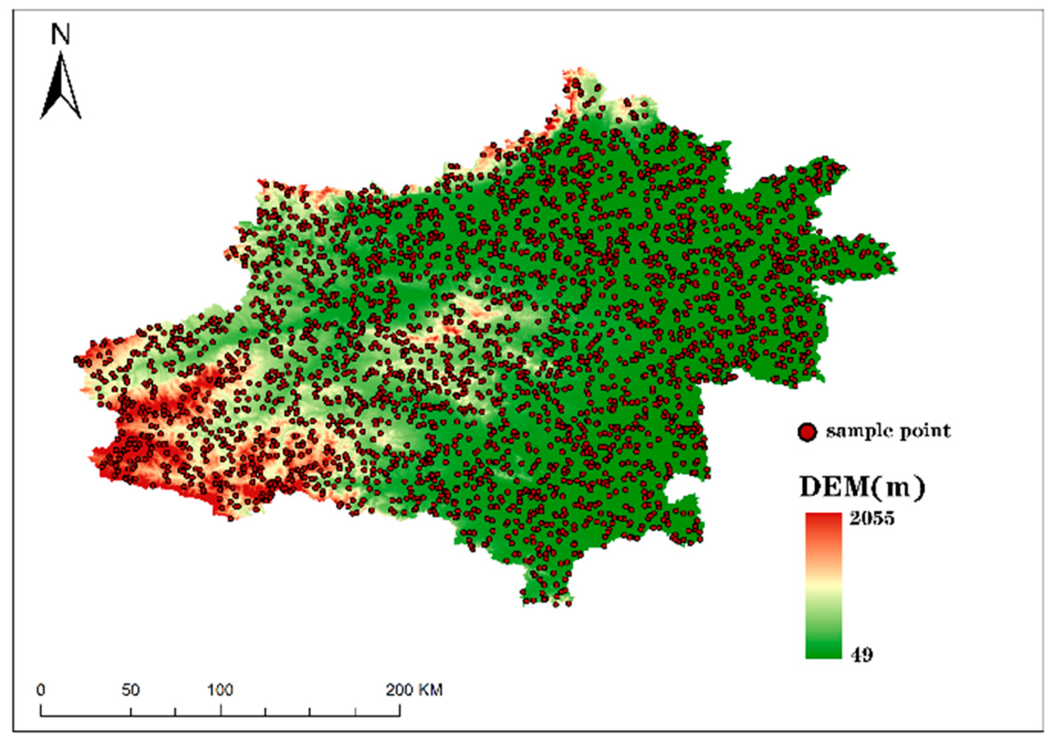
2.7.1. Sample Point Generation

In this study, 3,000 sample points were randomly generated within the Zhengzhou Metropolitan Area using ArcGIS 10.4, ensuring that no sample points were located within a 500m radius of each other. The landscape pattern indices and CS values were then extracted and associated with the corresponding sample points using the extraction tool. The extracted data were compiled into an attribute table linking the landscape pattern indices and CS in the study area. This table was subsequently exported to Excel for further analysis.

Figure 4. Distribution of the sample points (NO. GS (2022) 4308).

Figure 4. Distribution of the sample points (NO. GS (2022) 4308).

2.7.2. Correlation Analysis

In this study, SPSS 26.0 software was used to conduct a Spearman correlation analysis of landscape patterns and CS of urban BGSs in the study area at both the class level and landscape level. The correlation coefficient RRR represents the strength of the relationship between the data sets, ranging from -1 to 1. An R value between -1 and 0 indicates a negative correlation, suggesting a suppressive effect between the two data sets. Conversely, an R value between 0 and 1 indicates a positive correlation, implying a mutually enhancing effect between the two data sets. Additionally, the closer R is to -1 or 1, the stronger the correlation between the two variables. Specifically, an absolute value of the correlation coefficient RRR greater than 0.5 indicates a strong correlation; a value between 0.5 and 0.3 indicates a moderate correlation; a value between 0.3 and 0.1 indicates a weak correlation; and an RRR value less than 0.1 is generally considered to indicate weak or no correlation (Peng et al., 2018).

2.7.3. Regression Analysis

This study employed three regression methods—Ordinary Least Squares (OLS), GWR, and MGWR—to investigate the relationship between urban BGSP indices and CS.

OLS is a classic linear regression method used to analyze the impact of one or more independent variables on a dependent variable (Guo, 2021). GWR builds upon the classic linear regression model by accounting for the influence of spatial relationships on the regression model (Yang et al., 2022). However, GWR is limited by the assumption that all variables share the same optimal bandwidth, typically reflecting the average of the best bandwidth across all independent variables. In contrast, MGWR allows each independent variable to have its own bandwidth, thereby addressing the limitations of GWR. Compared to traditional GWR, MGWR enables each variable to exhibit distinct spatial smoothing levels, addressing the limitations of the GWR model (Ran, 2023), more accurately represents the true and useful spatial processes, and resulting in better model performance.

In this study, the performance of the three regression methods (OLS, GWR, and MGWR) is compared using R², Adj. R², and the corrected Akaike Information Criterion (AICc). A higher R² or adjusted R² value and a lower AICc indicate an improved regression model.

3. Results

3.1. Correlation Quantification Between BGSP Indices and CS

As shown in Figure 5, the total CS in the Zhengzhou Metropolitan Area is 1112.27×10⁶ t. The results of the quantified BGSPs are presented in Figure 6 and Figure 7.

Figure 5. Spatial distribution of CS in Zhengzhou Metropolitan Area (NO. GS (2022) 4308).

Figure 5. Spatial distribution of CS in Zhengzhou Metropolitan Area (NO. GS (2022) 4308).

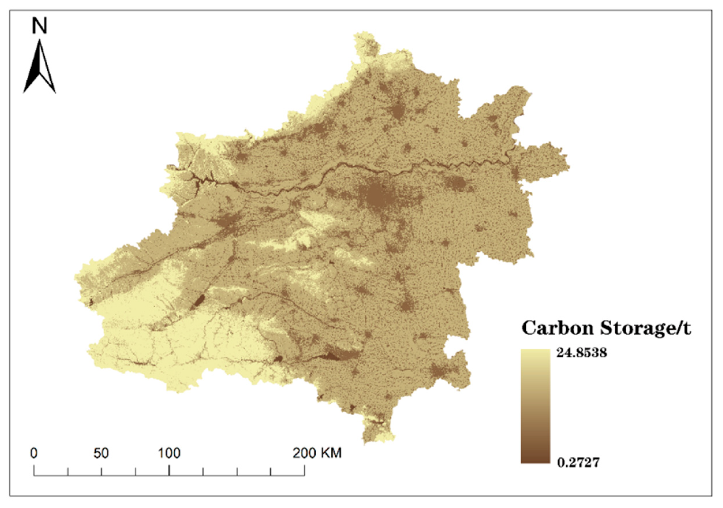
Figure 6. Class level of the BGSP incies.

Figure 6. Class level of the BGSP incies.

Figure 7. Landscape level of the BGSP indices.

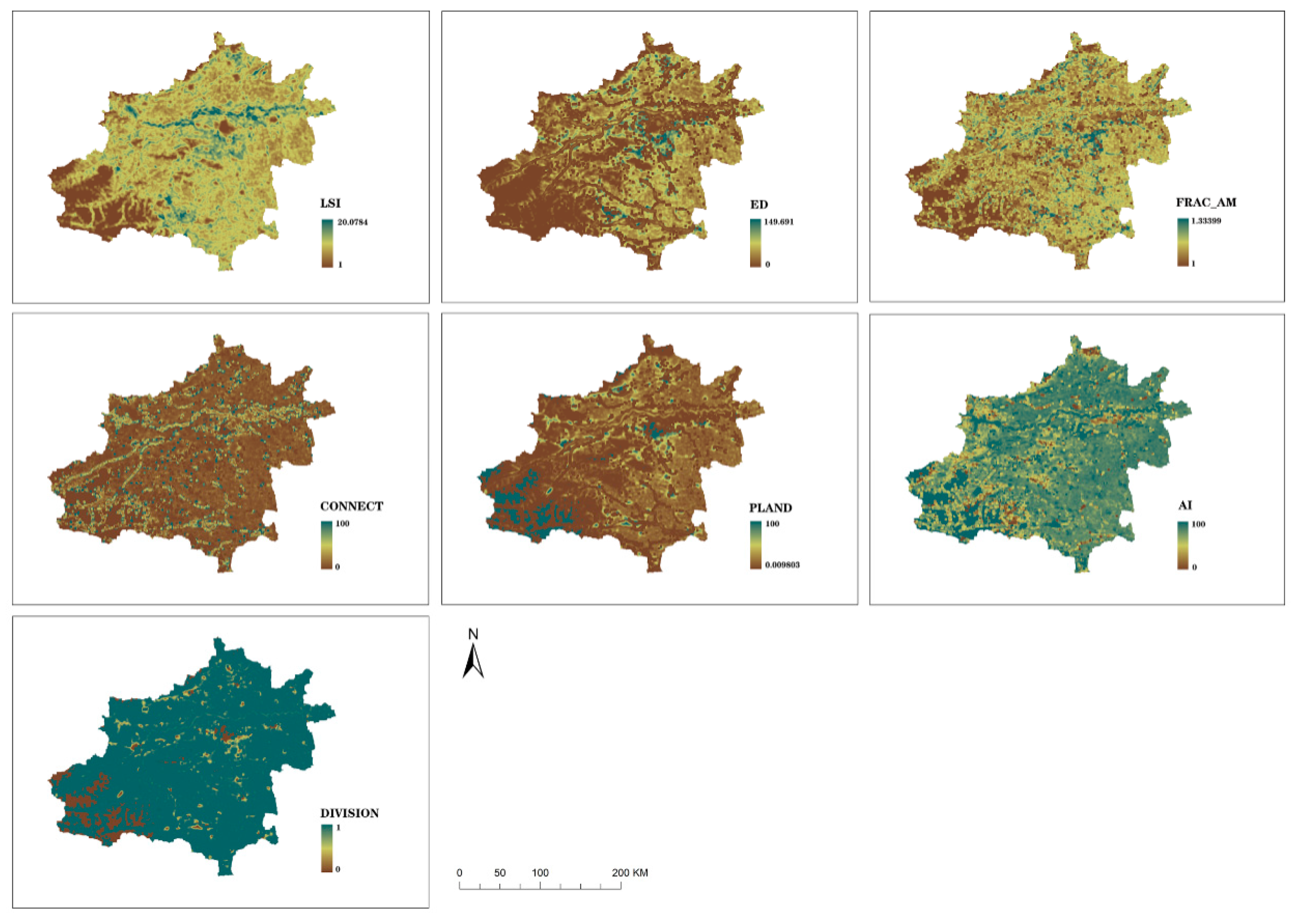
Figure 7. Landscape level of the BGSP indices.

At the class level, the correlations between BGSP indices and carbon storage (CS) exhibit multidimensional variations. In the Area-edge dimension, PLAND shows a weak negative correlation with CS (∣R∣=0.129, P<0.001), this might be because cropland, as a low-carbon vegetation type serving as the dominant patch, would suppress overall carbon storage when its area expands; ED demonstrates a moderate negative correlation (∣R∣=0.331, P<0.001), high edge density exacerbates landscape fragmentation, triggering microclimate changes and the loss of core habitats, thereby hindering the growth of high-carbon vegetation. In the Shape complexity dimension: LSI shows a moderate negative correlation with CS (∣R∣=0.427, P<0.001), More intact and stable ecological spaces are more conducive to carbon storage;FRAC_AM indicates a weak negative correlation (∣R∣=0.297, P<0.001), this suggests that complex and fragmented patch boundaries are highly susceptible to urban encroachment. In the Aggregation dimension, CONNECT have weak negative correlations with CS (∣R∣=0.199, P<0.001) ; DIVISION have weak negative correlations with CS (∣R∣=0.132, P<0.001), this indicates that high separation reduces connectivity between patches in the landscape, hinders the flow of matter and energy between ecosystems, and impacts carbon storage. While AI shows no correlation.

At the landscape level, In the Area-edge dimension, the strong negative correlation of ED (|R|=0.616, P<0.0001) highlights fragmentation’s inhibitory effect on carbon storage, whereas the strong positive correlation of LPI (|R|=0.618, P<0.0001) arises from large contiguous patches (e.g., intact forests) preserving soil carbon pools and stable microclimates. In the Shape complexity dimension, COHESION shows a strong positive correlation with CS (∣R∣=0.558, P<0.0001), This further demonstrates that the synergistic integration of blue-green spaces enhances carbon storage capacity, while CONTAG (∣R∣=0.342, P<0.0001) reflects moderate benefits from aggregated patches resisting disturbances. In the Connectivity dimension, CONNECT has a weak correlation with CS (∣R∣=0.150, P<0.0001). In the Diversity dimension, the strong negative correlation of SHDI (|R|=0.635, P<0.0001) implies that anthropogenic patch diversity degrades carbon sinks, whereas SHEI (|R|=0.602, P<0.0001) exhibits a strong positive correlation by balancing patch distributions to enhance functional complementarity (e.g., forest-wetland synergies). Exceptions include CONNECT (|R|=0.150, P<0.0001), whose weak negative correlation may stem from pest-driven collapses in monoculture plantations.

Table 5. Spearman correlations between CS and class-level indices.

	Indicators	PLAND	LSI	FRAC_AM	ED	DIVISION	CONNECT	AI
CS	Spearman.	-0.129**	-0.427**	-0.297**	-0.344**	0.132**	-0.199**	-0.084**
	Sig.	0.000	0.000	0.000	0.000	0.000	0.000	0.000

Table 5. Spearman correlations between CS and class-level indices.

	Indicators	PLAND	LSI	FRAC_AM	ED	DIVISION	CONNECT	AI
CS	Spearman.	-0.129**	-0.427**	-0.297**	-0.344**	0.132**	-0.199**	-0.084**
	Sig.	0.000	0.000	0.000	0.000	0.000	0.000	0.000

Table 6. Spearman correlations between CS and landscape-level indices.

	Indicators	SHDI	SHEI	LPI	ED	CONTAG	CONNECT	COHESION
CS	Spearman.	-0.635**	0.602**	0.618**	-0.616**	0.342**	-0.150**	0.588**
	Sig.	0.000	0.000	0.000	0.000	0.000	0.000	0.000

Table 6. Spearman correlations between CS and landscape-level indices.

	Indicators	SHDI	SHEI	LPI	ED	CONTAG	CONNECT	COHESION
CS	Spearman.	-0.635**	0.602**	0.618**	-0.616**	0.342**	-0.150**	0.588**
	Sig.	0.000	0.000	0.000	0.000	0.000	0.000	0.000

3.2. Comparative Analysis of Model Regression Results

The results show that the MGWR model performs better than the other models in several key indicators. At the class level: The R² value of MGWR is 0.505, and the adjusted R² is 0.447, which is higher than that of GWR (with R²=0.468, adjusted R²=0.425) and OLS (with R2=0.256, adjusted R2=0.254). The AICc of MGWR is 6535.135, lower than that of GWR (AICc=6453.154) and OLS (AICc=7051.910). At the landscape level, The R² value of MGWR is 0.484, and the adjusted R² is 0.414, which is higher than that of GWR (with R²=0.391, adjusted R2=0.339) and OLS (with R²=0.183, adjusted R²=0.181). The AICc of MGWR is 7124.151, lower than that of GWR (AICc=7307.537) and OLS (AICc=7663.153).

In summary, these results demonstrate that the MGWR model exhibits superior regression performance compared to the GWR and OLS models, effectively capturing the relationship between BGSP indices and CS.

Table 7. Regression results of models.

Level name	Indicators	OLS	GWR	MGWR
class	R2	0.256	0.468	0.505
	Adj. R2	0.254	0.425	0.447
	AICc	7051.910	6556.764	6535.135
landscape	R2	0.383	0.391	0.484
	Adj. R2	0.183	0.339	0.414
	AICc	7663.153	7307.537	7124.151

Table 7. Regression results of models.

Level name	Indicators	OLS	GWR	MGWR
class	R2	0.256	0.468	0.505
	Adj. R2	0.254	0.425	0.447
	AICc	7051.910	6556.764	6535.135
landscape	R2	0.383	0.391	0.484
	Adj. R2	0.183	0.339	0.414
	AICc	7663.153	7307.537	7124.151

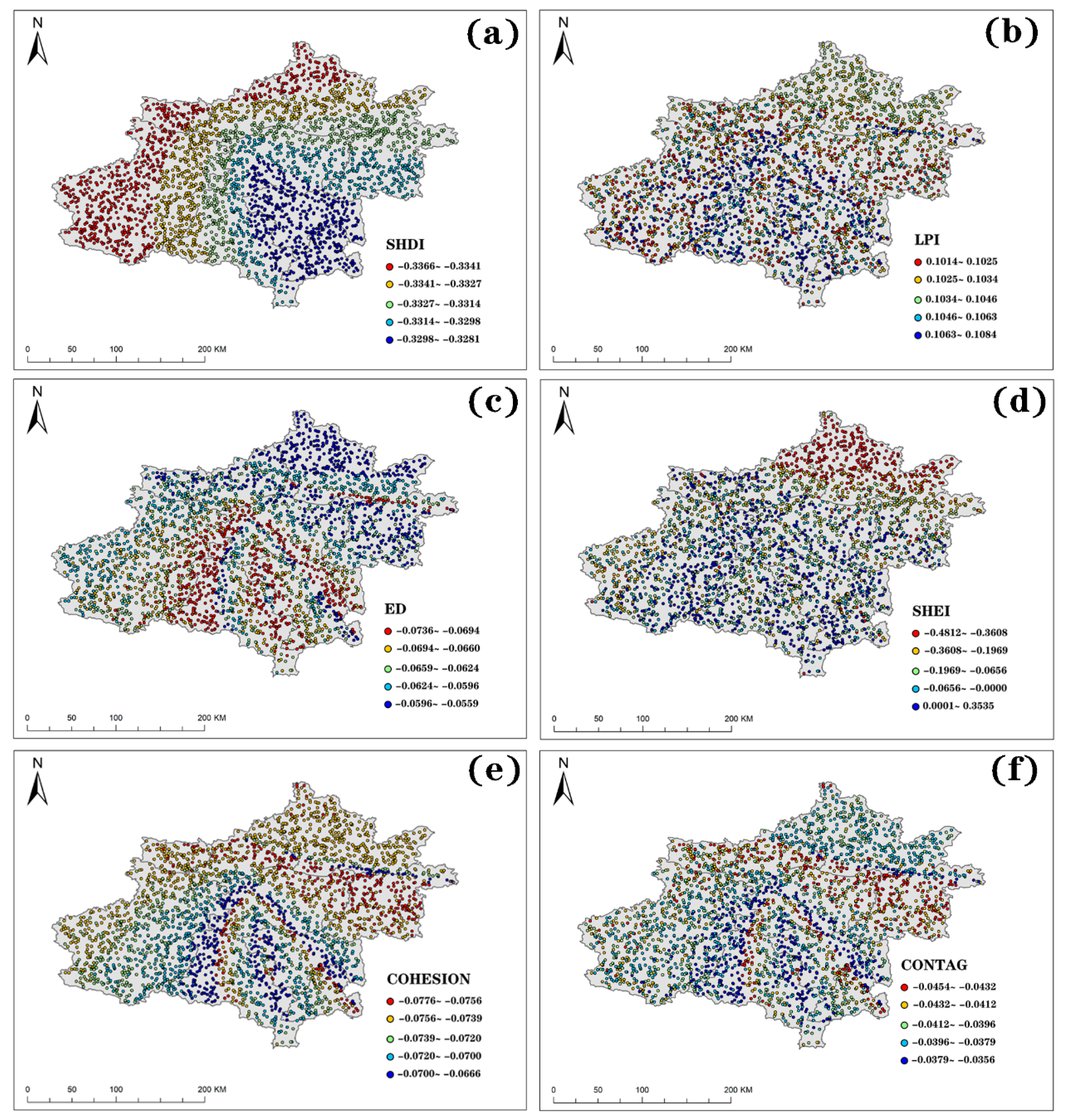
3.3. Spatial Heterogeneity in the Impact of BGSP on CS

This study selected four landscape pattern indices—LSI, ED, FRAC_AM, and CONNECT that have a high correlation with CS at the class level and visualized their MGWR regression coefficients spatially. The steps are as follows: calculating each coefficient in MGWR, importing the results into Excel to filter the variables for visualization, and then using the natural breaks method in ArcGIS 10.8 to classify the coefficients into five categories, thereby visualizing the coefficient patterns for each landscape index in the MGWR model.

Figure 7. Spatial pattern of regression coefficients of MGWR models at class level.

Figure 7. Spatial pattern of regression coefficients of MGWR models at class level.

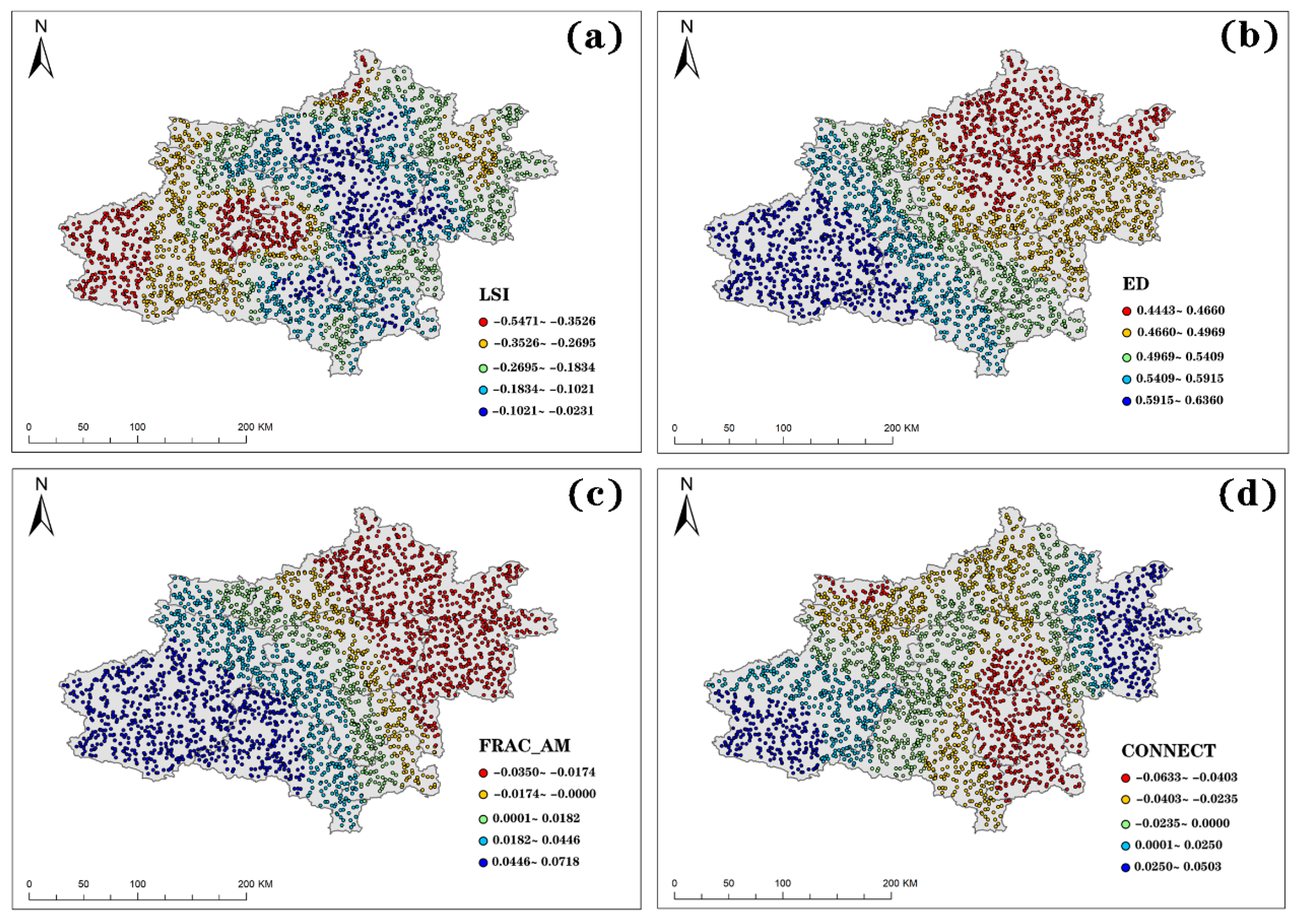
Figure 7 illustrates the distribution of the coefficient patterns for the landscape indices LSI, ED, FRAC_AM, and CONNECT at the class level in the MGWR model. It can be observed that each index exhibits spatial heterogeneity, with varying degrees of heterogeneity among the indices. LSI (Figure 7a): LSI shows a negative correlation with CS overall, with the coefficient pattern displaying a relatively uniform block-like spatial distribution. Higher correlations are found in areas dominated by forest land, while lower correlations are observed in areas dominated by built-up land. ED (Figure 7b): The influence of ED on CS is positive, with the coefficient pattern increasing from southeast to northwest, similar to the elevation gradient. FRAC_AM (Figure 7c): The impact of FRAC_AM on CS is not significant but shows both positive and negative variations. Negative impacts are observed in regions like Xinxiang, Kaifeng, Jiaozuo, Xuchang, and the north-eastern part of Zhengzhou, while positive influences are primarily seen in Luoyang, Pingdingshan, and Jiyuan. CONNECT (Figure 7d): The influence of CONNECT on CS is low, but its coefficient pattern is block-like. Overall, CONNECT positively influences the north-eastern and southwestern parts of the Zhengzhou Metropolitan Area, while having a negative influence in more central cities such as Zhengzhou and Xuchang.

Using the same method, the coefficients of landscape indices at the landscape level in the MGWR model were visualized. Figure 8 illustrates the distribution of coefficient patterns for landscape indices SHDI, LPI, ED, SHEI, COHESION, and CONTAG in the MGWR model at the landscape level, with each index still exhibiting strong spatial heterogeneity. SHDI (Figure 8a) has a negative impact on CS, with its influence generally displaying a banded distribution. The highest points are located in the northwest of Luoyang, as well as in Jiaozuo, Jiyuan, and northern Xinxiang, while the lowest points are found in cities such as Xuchang and Luohe. The influence of LPI (Figure 8b) on CS shows little variation with spatial changes but remains relatively low in the overall north-eastern direction, particularly in the Xinxiang area. The relationship between ED (Figure 8c) and CS remains negative at the landscape level, with the lowest points located in Xinxiang and Kaifeng. The higher points exhibit a radial distribution, with several banded high-impact areas emanating from Zhengzhou. The influence of SHEI (Figure 8d) on CS is more complex. In the north-eastern part of the Zhengzhou Metropolitan Area, it has a negative impact and the highest level of influence, while in other cities, the layout is mostly uniform and negatively influenced, with some areas showing a slight positive impact. Both COHESION (Figure 8e) and CONTAG (Figure 8f) have a relatively small impact on CS, with minimal variation in influence across different spatial areas.

Figure 8. Spatial pattern of regression coefficients of MGWR models at landscape level.

Figure 8. Spatial pattern of regression coefficients of MGWR models at landscape level.

4. Discussion

4.1. Key Indicators of BGSP Affecting CS

This study explored the relationship between urban BGSP and CS. We utilized OLS, GWR, and MGWR to analyze the effects of BGSP on CS at both global and local levels. The findings indicate that many indicators of urban BGSP are correlated with CS in urban ecosystems. Additionally, the influence of BGSP on CS exhibits spatial heterogeneity, demonstrating varying intensities of impact across different geographic locations. At the class level, PLAND, LSI, FRAC_AM, ED, CONNECT, and AI negatively affect CS. In contrast, DIVISION has a positive effect. At the landscape level, SHDI, ED, and CONNECT have a negative impact on CS, while SHEI, LPI, CONTAG, and COHESION exhibit positive influences. In Teng's research(Fei et al., 2022), it was found that the LSI in the Yangtze River Delta urban agglomeration is significantly negatively correlated with the carbon budget. The complex patch shape reduces the carbon sequestration capacity through the edge effect. This is probably because the serrated boundary of forest patches expands the edge area, leading to microclimate fluctuations, which in turn inhibits the photosynthesis of vegetation. In Peng's research(Peng et al., 2018), it was found that the Edge Density (ED), Average Patch Shape Index (SHAPE_MN) are positively correlated with carbon sequestration. these studies are similar to the research of this paper.

In patch morphology optimization, priority should be given to simplifying patch boundaries (reducing LSI) to minimize microclimate fluctuations caused by jagged edges, thereby enhancing vegetation photosynthetic efficiency. Concurrently, the establishment of ecological buffer zones can scientifically regulate patch connectivity, balancing the prevention of excessive sprawl with the maintenance of essential material exchange. Furthermore, oversized single patches may be appropriately subdivided (increasing DIVISION) to enhance spatial heterogeneity. This approach preserves core ecological stability while stimulating carbon storage potential through diversified habitats. In overall spatial planning, focus should center on high-carbon-sink landscape types such as forests and wetlands. Expanding core patch sizes (elevating LPI) can create contiguous dominant areas. Simultaneously, a hierarchical network should be established, characterized by "large patches as anchors and small patches as interconnected nodes," leveraging ecological corridors to boost material cycling efficiency. Additionally, enhancing patch aggregation (COHESION) and internal connectivity is critical to mitigate human-induced fragmentation of plant communities, ultimately providing a stable spatial framework for carbon storage processes.

4.2. The Impact of BGS Coupling on CS

At the class level emphasizing spatial integration, LSI has a negative impact on CS. This indicates that the more complex the shape of landscape patches, the less favorable it is for CS when the area of blue-green space is constant. This finding aligns with the research of Zhang (Zhang et al., 2024b), suggesting that simpler shapes in blue-green spaces are more beneficial for CS. This may be related to the combined influence of LSI and land use changes on CS. As shown in Figure 7a, areas with high LSI impacts are primarily located in forested regions, while those with lower impacts are in impervious areas. Therefore, prioritizing the integrity of forests in the Zhengzhou Metropolitan Area while reducing LSI is more favorable for CS than focusing solely on BGSs in urban settings. ED positively influences CS, and its impact decreases from the southwest to the northeast within the study area. This suggests that increasing the contact area of BGSs is more conducive to CS. For the same area, meandering shorelines and additional small water bodies, such as rain gardens and wetlands, are more beneficial for CS. The FRAC_AM of BGSs has a suppressive effect on CS in the northeastern part of the Metropolitan Aare (including Xinxiang, Kaifeng, northeastern Zhengzhou, and northeastern Xuchang), while promoting effects are observed in other areas. This may be related to the types of land use and elevation. Therefore, in cities like Luoyang and Pingdingshan, increasing the shape complexity of BGSs is advisable, while in Xinxiang and Kaifeng, simplifying the composition of BGSs can jointly enhance CS. The overall impact of CONNECT on CS is not high, but it has a positive influence in the western (Luoyang) and eastern (Xinxiang, Kaifeng) regions of the Zhengzhou Metropolitan Area, while negative impacts are observed in Zhengzhou, Xuchang, and Jiaozuo. This may be due to the higher connectivity of BGSs in western Luoyang and eastern Xinxiang and Kaifeng, which also correlates with higher CS levels. Conversely, in areas dominated by built-up land, lower connectivity of BGSs corresponds to lower CS, leading to different impacts. This indicates that in areas where BGSs are scarce and fragmented (such as those with a high proportion of impervious surfaces), it is beneficial for CS to maintain the area of BGSs while reducing their connectivity and forming a more integrated BGS. In contrast, in areas where BGSs are dominant (such as large forested areas and farmland), enhancing connectivity and forming a more complete BGS is more advantageous for CS.

4.3. Spatial Heterogeneity in the Impact of the Overall BGSP on CS

At the landscape level emphasizing the overall configuration of BGS, SHDI negatively impacts CS, showing a decreasing trend from northwest to southeast. While higher richness is generally believed to lead to greater carbon sinks, this study presents a different perspective. This discrepancy may be due to the larger scale of the study, where CS and carbon sinks in forested areas are higher than in other regions. Therefore, increasing SHDI in forest-dominated areas may negatively impact CS. This also indicates that prioritizing the integrity of large green spaces, such as forest parks and nature reserves, is more beneficial for CS. SHEI predominantly negatively influences CS, with the strongest impact observed in areas like Xinxiang, while other regions show little spatial variation. In contrast, research by Cao et al. (2024) indicates that SHDI can have alternating positive and negative effects on CS. LPI reflects the impact of the proportion of BGSs on CS, overall having a promoting effect. The distribution of high impact levels is relatively scattered, mainly concentrated in the central, southern, and western regions of Zhengzhou Metropolitan Area, suggesting that increasing the proportion of BGSs in these areas can achieve optimal CS enhancement. At the landscape level, ED has a suppressive effect on CS, which differs from its effect at the class level. This suggests that when BGSs are considered as a whole, a more gradual transition between natural areas and impervious surfaces is more conducive to CS. In contrast, when the internal composition of BGSs is more complex, it favors CS. This necessitates differentiated planning and design strategies for urban development based on varying BGS conditions. COHESION and CONTAG reveal the impact of the aggregation characteristics of patch types in landscape patterns on CS. As shown in Figure 8a and Figure 8b, the clustered distribution of BGSs can exert a certain suppressive effect on CS, which contrasts with previous studies (Cao et al., 2024). However, it also indicates that compared to isolated distributions, the synergy of BGSs can lead to greater CS accumulation. This highlights the need to emphasize the integrated development and coordinated planning of BGSs in urban planning.

4.4. Limitations and Prospects

This study utilized the InVEST model to estimate CS. While this model offers advantages such as low consumption and ease of calculation, it also has limitations, including relatively low accuracy and the assumption of identical CS for the same land use type. These limitations can affect the precision of regression analysis. Future research could further refine CS estimates by combining field surveys with modeling approaches. Additionally, it is generally believed that simply adjusting the structural morphology from a physical standpoint is insufficient to promote the growth of BGSs and, consequently, the accumulation of biomass to increase urban CS. However, changes in the structure of BGSs can enhance their interaction with natural environments, affecting aspects such as ventilation and light exposure, which in turn influences vegetation. Some studies have indicated that alterations in BGSPs can impact land surface temperature (LST) (He et al., 2024), while other research has confirmed that LST has a significant influence on carbon sinks (Lu et al., 2021). This suggests an intrinsic mechanism by which BGSPs affect CS. This study has initially explored the spatial mechanisms by which BGSPs influence CS. Future research may delve deeper into the underlying factors affecting these impacts.

5. Conclusions

This study explored the relationship between urban BGSPs and CS, identified the influencing factors of urban BGSPs on CS, and proposed planning and design recommendations. Based on land use data, the distribution of BGSs in Zhengzhou Metropolitan Area was determined, and the InVEST model was employed to calculate CS. By establishing indicators for urban BGSPs and conducting correlation analysis and MGWR model regression, this research established the numerical values of CS and the correlation between the overall and internal landscape patterns of blue-green spaces, as well as their key indicators. It quantified the spatial relationship between BGSPs and CS, thereby revealing the spatial mechanisms of their influence.

Further, from the perspective of optimizing urban BGSs to enhance CS in urban ecosystems, this study provides insights into the planning and layout of BGSs. This contributes to the systematic optimization of green space spatial patterns and offers new insights for urban planning and resource management practices, facilitating progress towards the “dual carbon” goals. Based on this, the following conclusions are drawn:

• There is a correlation between urban BGSPs and CS. The study indicates that when BGSs are considered as independent entities, simpler shape compositions and lower connectivity are more conducive to CS. However, when the synergistic effects of BGSs are taken into account, more tightly integrated, uniformly distributed, and less fragmented BGSs are more beneficial for CS.
• Comparative analysis revealed that the MGWR regression results are superior, indicating that the relationship between urban BGSPs and CS varies across different regions and exhibits significant spatial heterogeneity.
• In the planning and construction of BGSs within the Zhengzhou Metropolitan Area, the integrated development of these spaces plays a significant role in achieving the “dual carbon” goals. Enhancing the carbon sequestration capacity of BGSs can be achieved by increasing their contact frequency and reducing their degree of fragmentation. Furthermore, prioritizing interventions in areas where BGSs are predominant is more advantageous for CS.

References

- ALAM, SA, STARR, CLARK & BJF 2013. Tree biomass and soil organic carbon densities across the Sudanese woodland savannah: A regional carbon sequestration study. J ARID ENVIRON, 2013,89, 67-76.
- ALMAAITAH, T., APPLEBY, M., ROSENBLAT, H., DRAKE, J. & JOKSIMOVIC, D. 2021. The potential of blue-Green infrastructure as a climate change adaptation strategy: a systematic literature review. Blue-Green Systems. [CrossRef]
- BERA, B., BHATTACHARJEE, S., SENGUPTA, N., SHIT, P. K., ADHIKARY, P. P., SENGUPTA, D. & SAHA, S. 2022. Significant reduction of carbon stocks and changes of ecosystem service valuation of Indian Sundarban. Scientific Reports, 12. [CrossRef]
- CAO, H., WU, Z. & ZHENG, W. 2024. Impact of touristification and landscape pattern on habitat quality in the Longji Rice Terrace Ecosystem, southern China, based on geographically weighted regression models. Ecological Indicators, 166. [CrossRef]
- CHEN, L., WANG, X., CAI, X., YANG, C. & LU, X. 2022. Combined Effects of Artificial Surface and Urban Blue-Green Space on Land Surface Temperature in 28 Major Cities in China. Remote Sensing, 14. [CrossRef]
- CHEN, W., XIAO, D. & LI, X. 2002. [Classification, application, and creation of landscape indices]. Ying yong sheng tai xue bao = The journal of applied ecology / Zhongguo sheng tai xue xue hui, Zhongguo ke xue yuan Shenyang ying yong sheng tai yan jiu suo zhu ban, 13, 121.
- COX, P. M., PEARSON, D., BOOTH, B. B., FRIEDLINGSTEIN, P., HUNTINGFORD, C., JONES, C. D. & LUKE, C. M. 2013. Sensitivity of tropical carbon to climate change constrained by carbon dioxide variability. Nature, 494, 341-344. [CrossRef]
- FANGHU, S., FENGMAN, F., WEILIN, H., HAO, L., JIAN, Y., LI, F. & YUQING, M. 2023. Analysis and prediction of carbon storage evolution in Anhui province based on PLUS and InVEST model. Journal of Soil and Water Conservation, 37, 151-158.
- GIARDINA, CHRISTIAN, P., RYAN, MICHAEL & G. 2000. Evidence that decomposition rates of organic carbon in mineral soil do not vary with temperature. Nature.
- GUANGSHUI, C., YUSHENG, Y., LEZHONG, L., XIBO, L., YUECAI, Z. & YIDING, Y. 2007. Research Progress on Belowground Carbon Allocation in Forests. Journal of Subtropical Resources and Environment, 34-42.
- GUO, G., WU, Z., CAO, Z., CHEN, Y. & ZHENG, Z. 2021. Location of greenspace matters: a new approach to investigating the effect of the greenspace spatial pattern on urban heat environment. Landscape Ecology, 36, 1533-1548. [CrossRef]
- HAN, Y., KANG, W. & SONG, Y. 2018. Mapping and Quantifying Variations in Ecosystem Services of Urban Green Spaces: A Test Case of Carbon Sequestration at the District Scale for Seoul, Korea (1975–2015). International Review for Spatial Planning & Sustainable Development, 6, 110-120. [CrossRef]
- HE, J., SHI, Y., XU, L., LU, Z. & FENG, M. 2024. An investigation on the impact of blue and green spatial pattern alterations on the urban thermal environment: A case study of Shanghai. Ecological Indicators, 158. [CrossRef]
- HE, Z., LEI, L., ZENG, Z.-C., SHENG, M. & WELP, L. R. 2020. Evidence of Carbon Uptake Associated with Vegetation Greening Trends in Eastern China. Remote Sensing, 12. [CrossRef]
- HUANG DUO, Y. F., WANG SIZHE, WEI HUIJIE & WANG SHIFU 2022. Research on the Pattern and Indicator System of Blue-Green Space in Territorial Spatial Planning. City Planning, 46, 18-31.
- LEMMA, B., WILLIAMS, S. & PAUSTIAN, K. 2021. Long term soil carbon sequestration potential of smallholder croplands in southern Ethiopia with DAYCENT model. Journal of Environmental Management, 294. [CrossRef]
- LI, K. R., WANG, S. Q. & CAO, M. K. 2003. Vegetation and soil carbon storage in China.
- LU, X.-Y., CHEN, X., ZHAO, X.-L., LV, D.-J. & ZHANG, Y. 2021. Assessing the impact of land surface temperature on urban net primary productivity increment based on geographically weighted regression model. Scientific Reports, 11. [CrossRef]
- MCGARIGAL, K. & MARKS, B. J. 1995. FRAGSTATS—Spatial Pattern Analysis Program for Quantifying Landscape Structure. USDA Forest Service - General Technical Report PNW, 351.
- PENG, J., JIA, J., LIU, Y., LI, H. & WU, J. 2018. Seasonal contrast of the dominant factors for spatial distribution of land surface temperature in urban areas. Remote Sensing of Environment, 215, 255-267. [CrossRef]
- RAN, P., HU, S., FRAZIER, A. E., YANG, S., SONG, X. & QU, S. 2023. The dynamic relationships between landscape structure and ecosystem services: An empirical analysis from the Wuhan metropolitan area, China. Journal of Environmental Management, 325. [CrossRef]
- SANCHEZ, F. G. & GOVINDARAJULU, D. 2023. Integrating blue-green infrastructure in urban planning for climate adaptation: Lessons from Chennai and Kochi, India. TERI information digest on energy and environment: TIDEE, 22, 87-87. [CrossRef]
- SUN, W. & LIU, X. 2019. Review on carbon storage estimation of forest ecosystem and applications in China. Forest Ecosystems, 7. [CrossRef]
- WANG, Z., LI, X., MAO, Y., LI, L., WANG, X. & LIN, Q. 2022. Dynamic simulation of land use change and assessment of carbon storage based on climate change scenarios at the city level: A case study of Bortala, China. Ecological Indicators, 134. [CrossRef]
- WU, J., HOU, Y. & CUI, Z. 2024. Coupled InVEST–MGWR modeling to analyze the impacts of changing landscape patterns on habitat quality in the Fen River basin. Scientific Reports. [CrossRef]
- WU, J. G. 2000. Landscape Ecology: Pattern, Process, Scale and Hierarchy.
- YANG, L., YU, K., AI, J., LIU, Y., YANG, W. & LIU, J. 2022. Dominant Factors and Spatial Heterogeneity of Land Surface Temperatures in Urban Areas: A Case Study in Fuzhou, China. Remote Sensing, 14. [CrossRef]
- YUAN, Y., TANG, S., ZHANG, J. & GUO, W. 2023. Quantifying the relationship between urban blue-green landscape spatial pattern and carbon sequestration: A case study of Nanjing's central city. Ecological Indicators, 154. [CrossRef]
- ZHANG, R., YING, J. & ZHANG, R. 2024a. Urban green and blue infrastructure: unveiling the spatiotemporal impact on carbon emissions in China's Yangtze River Delta. Environmental Science and Pollution Research, 31, 18512-18526.
- ZHANG, R., YING, J., ZHANG, R. & ZHANG, Y. 2024b. Urban green and blue infrastructure: unveiling the spatiotemporal impact on carbon emissions in China's Yangtze River Delta. Environmental Science and Pollution Research.
- ZHANG, X., WANG, J., YUE, C., MA, S. & WANG, L.-J. 2022. Exploring the spatiotemporal changes in carbon storage under different development scenarios in Jiangsu Province, China. Peerj, 10.
- ZHANG YING, L. X. W. Y. 2022. Analysis of the Potential of Forest Carbon Sinks in China under the Background of Carbon Peak and Carbon Neutrality. Journal of Beijing Forestry University, 44, 38-47.
- ZHAO, J., GUO, F., ZHANG, H. & DONG, J. 2024. Mechanisms of non-stationary influence of urban form on the diurnal thermal environment based on machine learning and MGWR analysis. Sustainable Cities and Society, 101. [CrossRef]
- ZHAO, X. Y., YU-XUAN, D. U., HUA, L. I. & WANG, W. J. 2021. Spatio-temporal changes of the coupling relationship between urbanization and ecosystem services in the Middle Yellow River. Journal of Natural Resources, 36, 13. [CrossRef]
- FEI, T., YANJUN, W., MENGJIE, W., SHAOCHUN, L., YUNHAO, L. & HENGFAN, C. 2022. Spatiotemporal coupling relationship between urban spatial morphology and carbon budget in Yangtze River Delta urban agglomeration. Acta Ecologica Sinica, 42, 9636-9650.
- PENG, J., JIA, J., LIU, Y., LI, H. & WU, J. 2018. Seasonal contrast of the dominant factors for spatial distribution of land surface temperature in urban areas. Remote Sensing of Environment, 215, 255-267.
Disclaimer/Publisher’s Note: The statements, opinions and data contained in all publications are solely those of the individual author(s) and contributor(s) and not of MDPI and/or the editor(s). MDPI and/or the editor(s) disclaim responsibility for any injury to people or property resulting from any ideas, methods, instructions or products referred to in the content. |
© 2025 by the authors. Licensee MDPI, Basel, Switzerland. This article is an open access article distributed under the terms and conditions of the Creative Commons Attribution (CC BY) license (http://creativecommons.org/licenses/by/4.0/).
Copyright: This open access article is published under a Creative Commons CC BY 4.0 license, which permit the free download, distribution, and reuse, provided that the author and preprint are cited in any reuse.