Quantitative Remote Sensing of Sulfur Dioxide Emissions from Industrial Plants Using Passive Fourier Transform Infrared (FTIR) Spectroscopy

1. Introduction

The development of industrial sectors such as energy, metallurgy, chemicals, textiles, and pharmaceuticals is accompanied by an increase in emissions of harmful substances into the atmosphere [1]. These pollutants not only degrade the quality of life but also pose a serious threat to health [2].

The detection and identification of gas pollutants play an important role in environmental monitoring. It allows for tracking their sources, assessing the degree of danger, and developing effective control methods [3]. Currently, infrared (IR) Fourier spectroscopy [4,5], electrochemical sensing [6], differential absorption lidars [7,8,9,10,11], differential optical absorption spectroscopy [12,13,14], non-dispersive IR spectroscopy [15,16], and others are used to monitor atmospheric pollution.

Modeling the spread of pollutants in the air includes various approaches that can be categorized based on their mathematical frameworks and scales of application. Gaussian models are based on the assumption that the pollutants are normally distributed in the atmosphere; for example, AERMOD (EPA) [17], ADMS (CERC) [18], and ISC3 [19]. Lagrangian models calculate the trajectories of individual pollution particles, accounting for wind and turbulence; for example, HYSPLIT (NOAA) [20], FLEXPART [21], CALPUFF [22]. Eulerian models consider the atmosphere by dividing it into cells, for each of which the transport equations are solved; for example, CMAQ (EPA) [23], CHIMERE (EC) [24], and WRF-Chem [25]. Empirical models describe the scattering of clouds of heavy gas released into the atmosphere near the land surface; for example, B and McQ [26,27], VDI Guidelines [28].

Lagrangian models effectively account for changing weather conditions and complex terrain by utilizing three-dimensional meteorological fields and adaptively calculating particle trajectories. This makes them suitable for modeling accidental emissions and long-range pollution transport. However, a significant limitation of these models is their poor suitability for accounting for complex chemical reactions in the atmosphere, due to the computational difficulties associated with interacting, independently moving particles. Typically, Lagrangian models implement only the simplest chemical processes, such as radioactive decay or first-order linear reactions, while photochemical cycles, secondary aerosol formation, and other complex transformations remain beyond their scope. To solve this problem, hybrid approaches that combine Lagrangian and Eulerian methods are often used, enabling the modeling of complex atmospheric processes.

In contrast, Eulerian models have several significant disadvantages. Their primary weakness is limited spatial resolution, which leads to the "smearing" of point emission sources (such as chimneys) across the cells of the computational grid. This is especially critical for local-scale tasks where precise spatial detail is important. Furthermore, these models require substantial computing resources to increase detail; for instance, halving the grid spacing leads to an eightfold increase in computational load. They are also highly sensitive to the quality of the meteorological data, as small inaccuracies in wind or temperature fields can result in significant forecast inaccuracies.

Gaussian models are widely used for calculating pollutant dispersion from industrial chimneys due to their optimal combination of accuracy, simplicity, and established validity. This study employs the Pasquill-Briggs model to simulate sulfur dioxide (SO₂) emissions from chimneys. This approach requires a minimal set of input data, making it convenient for operational emission spread calculations. Compared to more complex Eulerian or Lagrangian approaches, the Gaussian model demands an order of magnitude fewer computational resources and less time while maintaining sufficient accuracy for industrial facilities with stationary emission sources.

This paper explores the use of remote sensing measurements via Fourier transform infrared (FTIR) spectroscopy to estimate the SO₂ emission rate from the chimneys of metallurgical plants. The Pasquill-Briggs model is used to calculate the emission rate from the measured path-integrated gas concentrations. This application requires supplementary data on gas outlet conditions (e.g., chimney height, gas exit velocity, and wind speed) as well as atmospheric characteristics (such as stability and the degree of solar insolation).

2. Materials and Methods

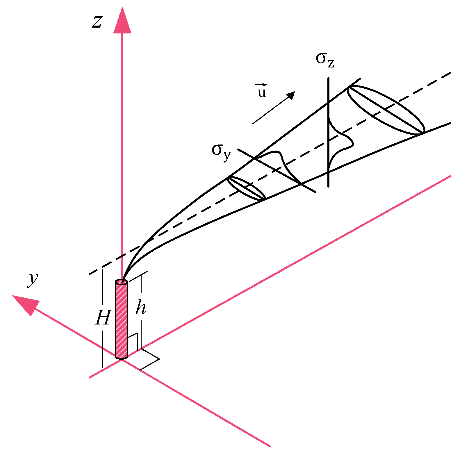
In this paper, we applied the Pasquill-Briggs model to estimate the flue gas distribution, and by solving the inverse problem, we were able to estimate the flue gas emission rate. The Pasquill-Briggs model describes the distribution of pollutants in the atmosphere as a Gaussian distribution. This approach is based on the turbulent diffusion equation with the following key assumptions [29,30]:

• dispersion in the horizontal and vertical planes is described by a Gaussian distribution with standard deviations ${\sigma }_y$ and ${\sigma }_z$ along the y and z axes, respectively;
• the average wind speed acting on the flow remains constant throughout the layer, and the wind direction does not change;
• the gas emission rate is constant;
• the flow can be reflected from the earth surface.

Taking these assumptions into account, the spatial distribution of the SO₂ concentration $c(x,y,z)$ from a point source with a constant wind directed along the x axis can be represented by the following formula within the framework of the Gaussian model (see Figure 1)

$$c(x,y,z)={\displaystyle \frac{q}{2\pi {\sigma }_y{\sigma }_{z}u}}exp{\displaystyle \frac{-y^2}{2{\sigma }_y^2}}\left(exp{\displaystyle \frac{-{(z-H)}^2}{2{\sigma }_z^2}}+exp{\displaystyle \frac{-{(z+H)}^2}{2{\sigma }_z^2}}\right),$$

(1)

where q is the gas emission rate [kg/s]; H is the height of the flare axis above ground level [m]; $\overrightarrow{u}$ is the horizontal wind speed along the torch axis [m/s]. In the Pasquill-Briggs model, the values of the scattering functions ${\sigma }_y$ and ${\sigma }_z$ are determined by the stability class of the atmosphere at a distance of 100 m to 10 km from the source. The stability class of the atmosphere is determined by wind speed, the degree of solar radiation, and cloud cover [31].

Taking into account the rise of the plume when modeling the dispersion of pollutants is critically important for the correct assessment of the effective height of the emission H, defined as the sum of the physical height of the source h and the vertical displacement of the plume $\Delta h$. For hot emissions characterized by significant buoyancy $(T_s\gg T_a)$, the rise of the plume is mainly due to thermal convection and is described by semi-empirical Briggs formulas [32]:

$$\Delta h=1.6{\displaystyle \frac{{\left(F_b{x}_c^2\right)}^{1/3}}{u}}\left[{\displaystyle \frac{2}{5}}+{\displaystyle \frac{16x}{25x_c}}+{\displaystyle \frac{11}{5}}{\left({\displaystyle \frac{x}{x_c}}\right)}^2\right]{\left(1+{\displaystyle \frac{4x}{5x_c}}\right)}^{-2},$$

(2)

where $F_b$ is a flux parameter [$m^4/s^3$]: $F_b=g{v}_s{r}^2\left({\displaystyle \frac{T_s-T_a}{T_s}}\right)$, $g=9.81$ – free fall acceleration [$m/s^2$]; $v_s=4.36$ – vertical speed [m/s]; $r=4.36$ – exit radius [m]; $T_s,T_a$ – the exit gas and ambient temperature [K]; $x_c=A{F}_b^{2/5}{h}^{3/5}$ – the distance downwind at which environmental turbulence begins to dominate the dispersion process is known as the critical distance [m]; $A=2.16$ [$s^{6/5}/m^{6/5}$].

The most important step in constructing the plume distribution is to obtain the initial parameters of the model. The basic meteorological parameters (wind speed, atmospheric stability class) required for calculations are set directly from the weather forecast at the time of the measurements. The path-integrated gas concentrations in the flux are calculated according to the direction of data recorded on the Fourier spectrometer. The emission rate q is calculated by comparing experimentally obtained path-integrated gas concentrations of pollutants $C_{int}^E(\theta ,\varphi )$ in the exhaust gas plume with the simulated values $C_{int}^T(\theta ,\varphi )$, where $\theta ,\varphi$ – the angle of location and azimuth relative to the observation point. The simulation of path-integrated gas concentrations was carried out as follows:

$$C_{int}^T(\theta ,\varphi )={\int }_0^{\infty }{c}_{sp}(r,\theta ,\varphi )dr,$$

(3)

where $c_{sp}(r,\theta ,\varphi )$ is calculated using the distribution $c(x,y,z)$, by switching to a spherical coordinate system with rotation and shifting the origin to the observation point. For the described transformations, additional parameters are introduced: the azimuth on the tube ${\theta }_s$ and the distance to the tube from the observation point $r_s$. By varying the direction of wind speed and emission rate q, the minimum discrepancy between the theoretical and experimentally measured series of values is determined:

$$\parallel C_{int}^T(\theta ,\varphi )-C_{int}^E(\theta ,\varphi )\parallel \stackrel{\overrightarrow{u},q}{\to }min$$

(4)

The desired value of the ejection power is determined from condition 4. The experimental concentrations were determined by remote sensing using an infrared Fourier spectrometer. Obtaining experimental values $C_{int}^E(\theta ,\varphi )$ is presented in detail in [1]. The efficiency of SO₂ detection in the infrared range of the spectrum has been shown in [1,33].

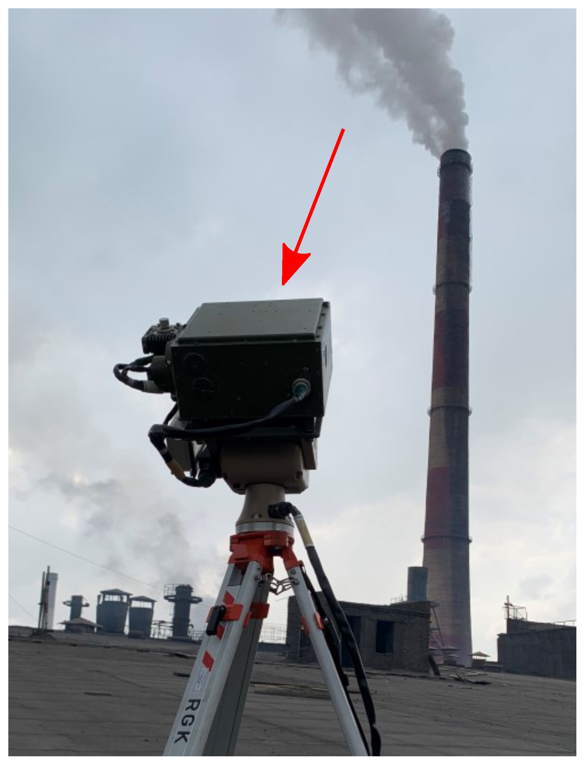
3. Experimental Setup

Figure 2 shows a diagram of an experiment on the remote recording of infrared chimney exhaust gas spectra. Table 1 shows the main technical characteristics of the infrared Fourier spectrometer. The Fourier spectrometer was located on an automated pan tilt positioner controlled via the ethernet protocol, with the ability to automatically transmit azimuth and elevation for each measurement, along with a time reference, which makes it possible to use the Pasquill-Briggs model to calculate emissions. The positioning accuracy of the automatic pan tilt positioner is at least 1 mrad.

4. Results and Discussion

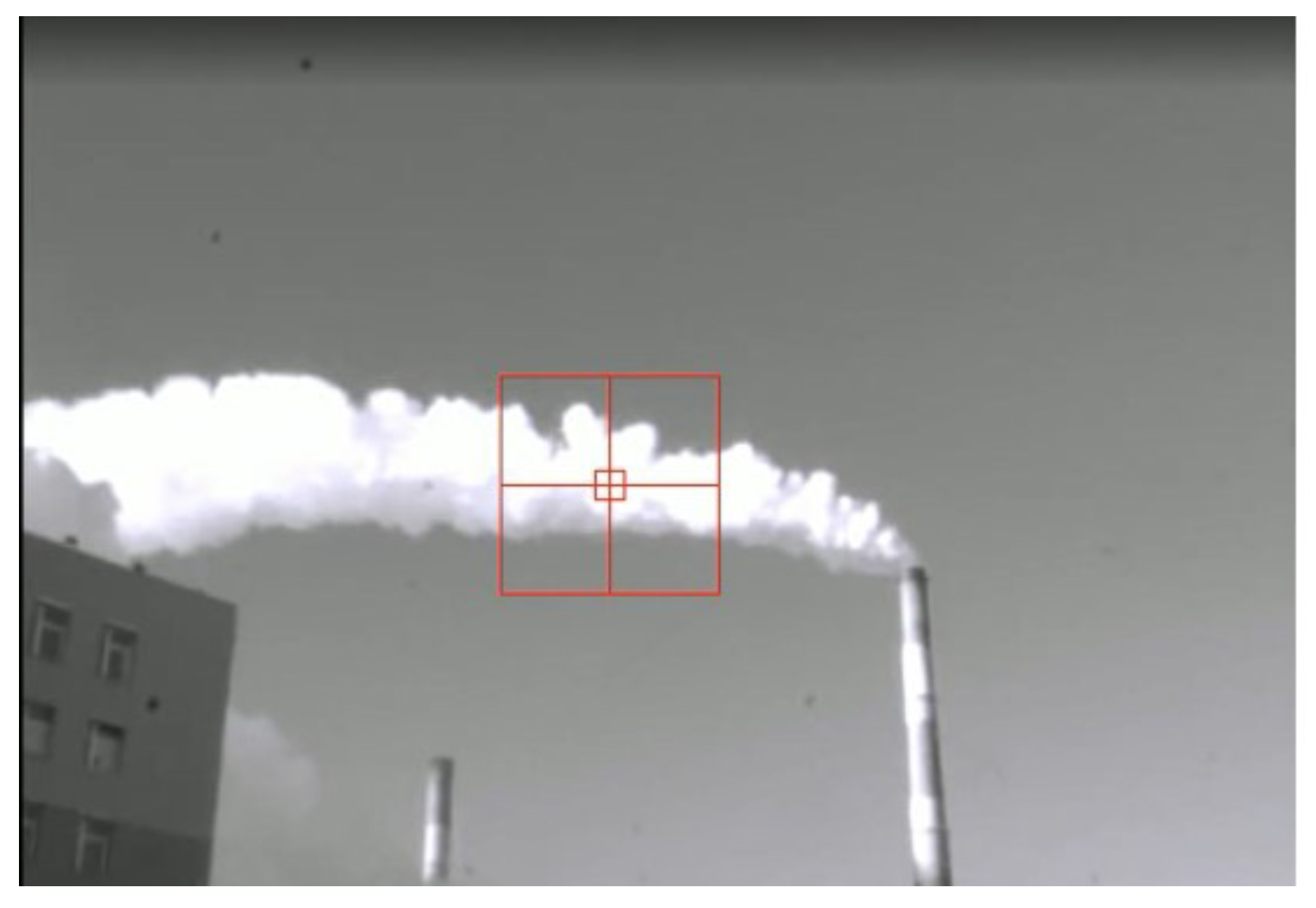
Measurements of path-integrated gas concentrations were carried out in two series. The series were held over two days, with each episode lasting 30 minutes. The measurement conditions, as well as the simulation parameters, are shown in Table 2. Figure 3 shows the side view of the plume from the spectrometer. The middle of the crosshair shows the axis of the infrared channel. The red square is shown conditionally. 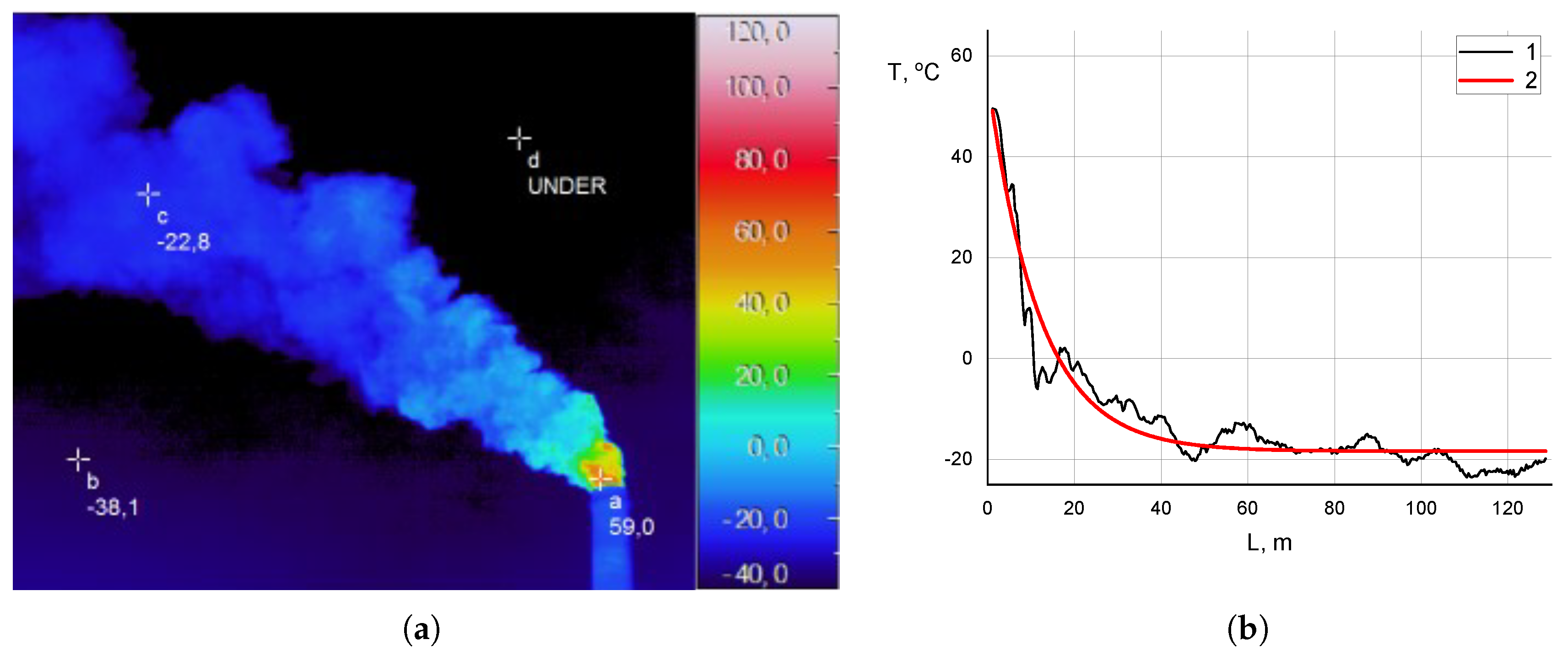Figure 4 shows an analysis of thermograms of exhaust plumes with an assessment of the temperature contrast.

Figure 4 shows the thermogram of the exhaust plume obtained using the NEC 2640 high-resolution thermal camera from the same position as the spectrometer. Figure 4 shows the temperature distribution along the plume from the chimney exit (L is the distance from the chimney exit, m). The thermogram shows that on the day of the measurement, the effective temperature of the underlying surface (sky) is $-38.1^{\circ }C$ or less, which corresponds to a temperature contrast between the exhaust plume and the underlying surface of the order of ${20}^{\circ }$ or more.

The measurement conditions given in Table 2 and Table 3 show the main parameters of the Pasquill-Briggs model. The results of the calculations of the point source plume propagation are shown in Figure 5, Figure 6 and Figure 7.

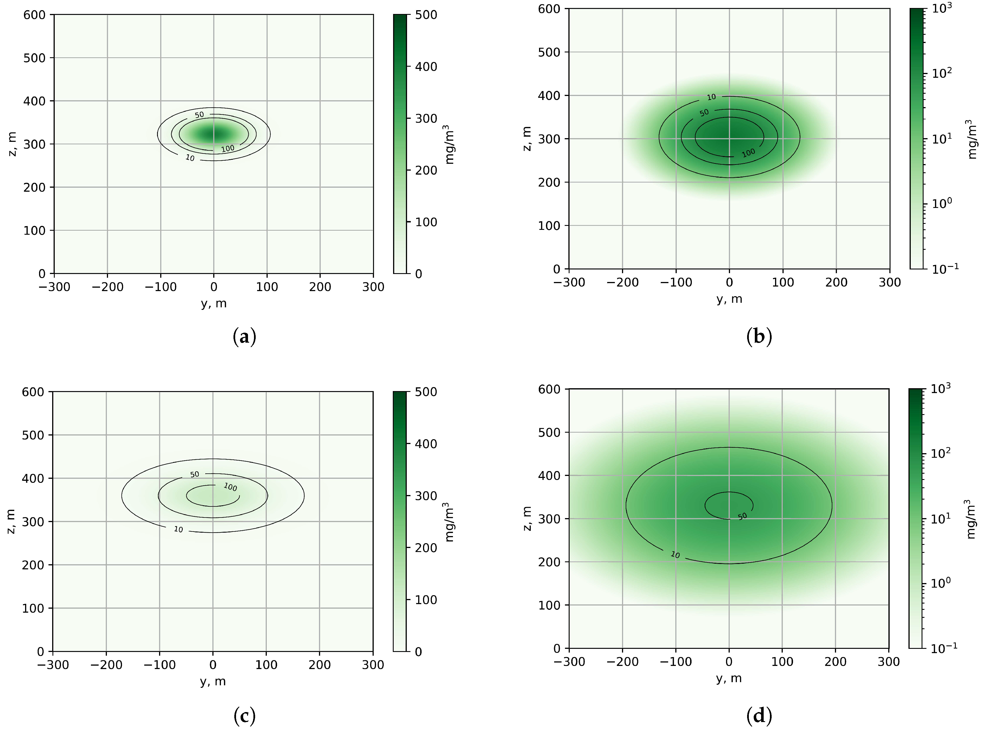
The graph shown (Figure 5) illustrates the vertical profile of the SO₂ distribution for various distances from the emission source, calculated using the data from the corresponding experiment No. 1. Near the source (no more than 1000 m), in the zone of active plume rise, the concentration distribution shows a symmetrical Gaussian character (Figure 6 and Figure 7) with a maximum located at an altitude determined by Formula (2).

The analysis of the concentration isolines demonstrates a characteristic expansion in the zone of maximum elevation, followed by a stabilized spread at altitudes of about 350-400 m. Data on the height of the plume rise in a specific location allow the spectrometer to be optimally positioned for the accurate targeting of the area of maximum concentration of pollutants. Knowledge of the vertical distribution of the plume ensures the correct selection of elevation and azimuth angles during scanning, which increases the reliability of measurements of path-integrated gas concentration and minimizes errors associated with the incomplete capture of the cross-section of the plume.

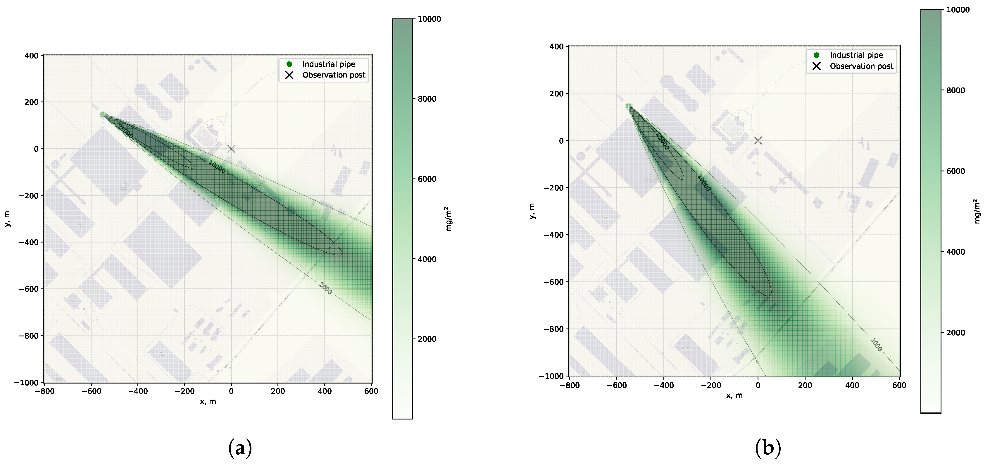
To choose the optimal location for the observation point, it is necessary to combine the terrain map with data on the density and direction of winds, as well as information on the distribution of pollution sources and possible obstacles. Preliminary data on wind and emission rates allow us to estimate the pollution density in advance and determine the most suitable location for an observation point.

When calculating the emission rate of n sources (chimneys), a linear superposition of the emissions from each individual source is applied simultaneously, taking into account the position of the sources on the terrain map $c(x,y,z)={\sum }_{i=1}^{n}c(x-x_i,y-y_i,z)$.

During series No. 1, 15 experiments were performed to register the IR spectra of SO₂ while scanning the FTIR spectrometer along the plume. During series No. 2, 25 measurements were performed. The results of the analysis of the two series are shown in Table 4.

Accurate emission data are not available for remote measuring, as it is difficult to obtain local monitoring by simultaneously measuring gas flows in all pipes entering the chimney. Another way to estimate the emission rate may be through PEMS (Predictive Emissions Monitoring Systems) models. However, the PEMS data are indirect and also require validation. The above errors in the emission rate are determined to be random errors, such as errors in registering IR spectra and in determining wind speed (especially the vertical component, where the error of anemometers reaches $\pm 5\%$), as well as methodological errors related to solving the multilayer problem of atmospheric optics for determining concentrations while considering atmospheric turbulence, etc.

5. Conclusions

This paper presents a methodology for the remote quantification of chimney emission rates from metallurgical plants. Remote optical techniques enable the acquisition of path-integrated gas concentration data across a plume’s cross-section, a parameter not accessible through conventional in-situ point sampling. The integration of such line-integrated measurements with atmospheric dispersion modeling allows for the comprehensive reconstruction of total substance flow. Specifically, the method employs ground-based Fourier transform infrared spectrometry to measure the path-integrated concentration within the gas flux. The FTIR spectrometer, operating in the mid-infrared range (7–14 $\mu m$) at a spectral resolution of 4 cm$--1$ and a scanning frequency of 1 Hz, was deployed at a distance of 570 m from the emission source.

The emission rates of sulfur dioxide were calculated using the Pasquill-Briggs Gaussian dispersion model. Model inputs included source parameters (chimney height, nozzle diameter, and gas exit velocity) and real-time meteorological data (wind speed and atmospheric stability class). Analysis of two distinct 30-minute measurement series, conducted on separate days, yielded average emission rates of 15.0 kg/s and 22.0 kg/s, with corresponding coefficients of variation of 45.2% and 32.8%. This level of uncertainty is consistent with established dispersion modeling approaches, which report inter-model discrepancies on the order of 35% for emission rate estimations [33].

The presented remote sensing approach provides a practical tool for estimating industrial emission fluxes. Furthermore, the derived data can serve as critical input for modeling the dispersion and transport of gaseous emissions in complex topographic environments.

References

- Morozov, A.N.; Tabalin, S.E.; Anfimov, D.R.; Vintaykin, I.B.; Glushkov, V.L.; Demkin, P.P.; Nebritova, O.A.; Golyak, I.S.; Barkov, E.V.; Chebotaev, A.V.; et al. Estimation of Emissions From Metallurgical Plants Using Infrared Fourier Transform Spectroscopy. Russian Journal of Physical Chemistry B 2024, 18, 763–772. [Google Scholar] [CrossRef]
- Donateo, A.; Villani, M.G.; Feudo, T.L.; Chianese, E. Recent Advances of Air Pollution Studies in Italy. Atmosphere 2020, 11, 1054. [Google Scholar] [CrossRef]
- Gaudio, P.; Gelfusa, M.; Malizia, A.; Parracino, S.; Richetta, M.; De Leo, L.; Perrimezzi, C.; Bellecci, C. Detection and monitoring of pollutant sources with Lidar/Dial techniques. Journal of Physics: Conference Series 2015, 658, 012004. [Google Scholar] [CrossRef]
- Golyak, I.S.; Anfimov, D.R.; Vintaykin, I.B.; Golyak, I.S.; Drozdov, M.S.; Morozov, A.N.; Svetlichnyi, S.I.; Tabalin, S.E.; Timashova, L.N.; Fufurin, I.L. Monitoring Greenhouse Gases in the Open Atmosphere by the Fourier Spectroscopy Method. Russian Journal of Physical Chemistry B 2023, 17, 320–328. [Google Scholar] [CrossRef]
- Mayorova, V.; Morozov, A.; Golyak, I.; Golyak, I.; Lazarev, N.; Melnikova, V.; Rachkin, D.; Svirin, V.; Tenenbaum, S.; Vintaykin, I.; et al. Determination of Greenhouse Gas Concentrations from the 16U CubeSat Spacecraft Using Fourier Transform Infrared Spectroscopy. Sensors 2023, 23, 6794. [Google Scholar] [CrossRef]
- Kau, N.; Jindal, G.; Kaur, R.; Rana, S. Progress in development of metal organic frameworks for electrochemical sensing of volatile organic compounds. Results in Chemistry 2022, 4, 100678. [Google Scholar] [CrossRef]
- Carlisle, C.B.; van der Laan, J.E.; Carr, L.W.; Adam, P.; Chiaroni, J.P. CO2 laser-based differential absorption lidar system forrange-resolved and long-range detection of chemical vapor plumes. Appl. Opt. 1995, 34, 6187–6200. [Google Scholar] [CrossRef]
- Li, J.; Yu, Z.; Du, Z.; Ji, Y.; Liu, C. Standoff Chemical Detection Using Laser Absorption Spectroscopy: A Review. Remote Sensing 2020, 12, 2771. [Google Scholar] [CrossRef]
- Yang, Z.h.; Zhang, Y.k.; Chen, Y.; Li, X.f.; Jiang, Y.; Feng, Z.z.; Deng, B.; Chen, C.l.; Zhou, D.f. Simultaneous detection of multiple gaseous pollutants using multi-wavelength differential absorption LIDAR. Optics Communications 2022, 518, 128359. [Google Scholar] [CrossRef]
- Innocenti, F.; Robinson, R.; Gardiner, T.; Finlayson, A.; Connor, A. Differential Absorption Lidar (DIAL) Measurements of Landfill Methane Emissions. Remote Sensing 2017, 9, 953. [Google Scholar] [CrossRef]
- Cezard, N.; Mehaute, S.L.; Gouët, J.L.; Valla, M.; Goular, D.; Fleury, D.; Planchat, C.; Dolfi-Bouteyre, A. Performance assessment of a coherent DIAL-Doppler fiber lidar at 1645 nm for remote sensing of methane and wind. Opt. Express 2020, 28, 22345–22357. [Google Scholar] [CrossRef] [PubMed]
- Johansson, M.; Galle, B.; Yu, T.; Tang, L.; Chen, D.; Li, H.; Li, J.; Zhang, Y. Quantification of total emission of air pollutants from Beijing using mobile mini-DOAS. Atmospheric Environment 2008, 42, 6926–6933. [Google Scholar] [CrossRef]
- Wang, S.; Zhou, B.; Wang, Z.; Yang, S.; Hao, N.; Valks, P.; Trautmann, T.; Chen, L. Remote sensing of NO2 emission from the central urban area of Shanghai (China) using the mobile DOAS technique. Journal of Geophysical Research: Atmospheres 2012, 117. [Google Scholar] [CrossRef]
- Tan, W.; Liu, C.; Wang, S.; Liu, H.; Zhu, Y.; Su, W.; Hu, Q.; Liu, J. Long-distance mobile MAX-DOAS observations of NO2 and SO2 over the North China Plain and identification of regional transport and power plant emissions. Atmospheric Research 2020, 245, 105037. [Google Scholar] [CrossRef]
- Vojtisek-Lom, M.; Zardini, A.A.; Pechout, M.; Dittrich, L.; Forni, F.; Montigny, F.; Carriero, M.; Giechaskiel, B.; Martini, G. A miniature Portable Emissions Measurement System (PEMS) for real-driving monitoring of motorcycles. Atmospheric Measurement Techniques 2020, 13, 5827–5843. [Google Scholar] [CrossRef]
- Sun, Q.; Liu, T.; Yu, X.; Huang, M. Non-interference NDIR detection method for mixed gases based on differential elimination. Sensors and Actuators B: Chemical 2023, 390, 133901. [Google Scholar] [CrossRef]
- Cimorelli, A.J.; Perry, S.G.; Venkatram, A.; Weil, J.C.; Paine, R.; Wilson, R.B.; Lee, R.F.; Peters, W.D.; Brode, R.W. AERMOD: A Dispersion Model for Industrial Source Applications. Part I: General Model Formulation and Boundary Layer Characterization. Journal of Applied Meteorology 2005, 44, 682–693. [Google Scholar] [CrossRef]
- Carruthers, D.; Holroyd, R.; Hunt, J.; Weng, W.; Robins, A.; Apsley, D.; Thompson, D.; Smith, F. UK-ADMS: A new approach to modelling dispersion in the earth’s atmospheric boundary layer. Journal of Wind Engineering and Industrial Aerodynamics 1994, 52, 139–153. [Google Scholar] [CrossRef]
- Petersen, W.B.; Perry, S.G. Improved Algorithms for Estimating the Effects of Pollution Impacts from Area and Open Pit Sources. In Air Pollution Modeling and Its Application XI; Springer US, 1996; pp. 379–388. [Google Scholar] [CrossRef]
- Stein, A.F.; Draxler, R.R.; Rolph, G.D.; Stunder, B.J.B.; Cohen, M.D.; Ngan, F. NOAA’s HYSPLIT Atmospheric Transport and Dispersion Modeling System. Bulletin of the American Meteorological Society 2015, 96, 2059–2077. [Google Scholar] [CrossRef]
- Stohl, A.; Forster, C.; Frank, A.; Seibert, P.; Wotawa, G. Technical note: The Lagrangian particle dispersion model FLEXPART version 6.2. Atmospheric Chemistry and Physics 2005, 5, 2461–2474. [Google Scholar] [CrossRef]
- Holnicki, P.; Kałuszko, A.; Trapp, W. An urban scale application and validation of the CALPUFF model. Atmospheric Pollution Research 2016, 7, 393–402. [Google Scholar] [CrossRef]
- Appel, K.W.; Bash, J.O.; Fahey, K.M.; Foley, K.M.; Gilliam, R.C.; Hogrefe, C.; Hutzell, W.T.; Kang, D.; Mathur, R.; Murphy, B.N.; et al. The Community Multiscale Air Quality (CMAQ) Model Versions 5.3 and 5.3.1: System Updates and Evaluation. Geoscientific Model Development 2020, 14, 2867–2897. [Google Scholar] [CrossRef]
- Terrenoire, E.; Bessagnet, B.; Pirovano, G.; Thunis, P.; Colette, A.; Ung, A.; Letinois, L.; Rouil, L. Evaluation of the chimere model at high resolution over Europe: focus on urban area. In Proceedings of the Proceedings of the 8th International Conference on Air Quality, Science and Application, Athènes, Greece, mar 2012; p. NC. [Google Scholar]
- Georgiou, G.K.; Christoudias, T.; Proestos, Y.; Kushta, J.; Pikridas, M.; Sciare, J.; Savvides, C.; Lelieveld, J. Evaluation of WRF-Chem model (v3.9.1.1) real-time air quality forecasts over the Eastern Mediterranean. Geoscientific Model Development 2022, 15, 4129–4146. [Google Scholar] [CrossRef]
- Britter, R.; Mcquaid, J. Workbook on the dispersion of dense gases. Technical report, Health and Safety Executive, 1988. [Google Scholar]
- Britter, R.E. Recent research on the dispersion of hazardous materials. Report EUR 18198 EN, Brussels, Belgium, 1998; Council of European Communities. [Google Scholar]
- Verein Deutscher Ingenieure (VDI). VDI 3783 Part 2: Environmental meteorology; dispersion of heavy gas emissions by accidental releases; safety study. Guideline Available in both German and English. 1990. [Google Scholar]
- Markiewicz, M. A Review of Mathematical Models for the Atmospheric Dispersion of Heavy Gases. Part I. A Classification of Models. Ecological Chemistry and Engineering S 2012, 19, 297–314. [Google Scholar] [CrossRef]
- Gifford, F.A. Use of routine meteorological observations for estimating atmospheric dispersion. Nuclear safety 1961, 2, 47–51. [Google Scholar]
- Briggs, G. Diffusion estimation for small emissions. Preliminary report. Technical report; Office of Scientific and Technical Information (OSTI), 1973. [Google Scholar] [CrossRef]
- Briggs, G. Chimney plumes in neutral and stable surroundings. Atmospheric Environment (1967) 1972, 6, 507–510. [Google Scholar] [CrossRef]
- Thepanond, S. Evaluation of dispersion model performance in predicting SO2 concentrations from petroleum refinery complex. International Journal of Geomate 2016. [Google Scholar] [CrossRef]