Submitted:
16 December 2025
Posted:
17 December 2025
You are already at the latest version
Abstract
Climate change poses significant risks to Mediterranean aquaculture, with sea surface temperature (SST) identified as a critical stressor affecting cultivated species. This study aims to assess climate-related risks for coastal aquaculture in the Valencian Community (Spain) by analyzing SST spatiotemporal variability and predicting future trends. A multi-method approach was employed, combining ARIMA models for 10-year predictions at eight coastal locations, Bayesian hierarchical models (BHM) fitted via INLA for spatiotemporal analysis of maximum SST and temperature range (2000–2024), and Generalized Additive Models (GAM) to evaluate relationships with climate indices (NAO, AMO, ENSO). Results revealed a consistent warming trend since the 1990s, with ARIMA predictions indicating maximum SST values of 27.2±0.1 °C in September over the next decade. The spatiotemporal model showed effective spatial correlation ranges of 246 km for maximum SST and 207 km for SST range. Anomalous warming years (2003, 2006, 2018, 2023–2024) coincided with documented marine heatwave events. The GAM explained 98.2% of deviance, with AMO showing significant influence (>0.001) while ENSO was not statistically significant. Notably, the area north of San Antonio Cape exhibited lower warming trends, suggesting potential climate refuge characteristics. Southern locations (Altea, Campello) currently experience the highest temperatures, but projections indicate Valencia and Sagunto will become the warmest areas. These findings provide essential information for marine spatial planning and recommend a precautionary approach when considering aquaculture relocation towards northern coastal areas.
Keywords:
time series
; ecosystems
; nonlinear methods
; short-term and long-term dynamics
; SST
; marine spatial planning
; climate change
1. Introduction
Achieving a smarter and sustainable aquaculture and fishing industry, equipped with technological advancements tailored to climate change and its monitoring, stands as a predominant objective in marine science research and development. The inadequate planning could become economically unsustainable due to climate stressors and the actual climate variances have impacted aquaculture production negatively around the world ([1]). There has been a notable increase in the amplitude of the daily sea surface temperature (SST) seasonal cycle over many ocean basins since 1950 ([2]). Also, many studies have tried to analyze these trends, highlighting that some areas are more vulnerable than others. Our area of interest, located in the Mediterranean Sea, is one of these sensitive regions ([3]). This region is recognized as the largest climate change hotspot, experiencing warming rates up to 20% higher than the global average ([4]).
In order to establish a better spatial planning for the sustaintable acuaculture, the Available Zones for Aquaculture (AZAs) defined by the FAO ([5]) summarize the main oceanographic features necessary for developing sustainable aquaculture along the Mediterranean coast. However, under a climate change scenario, these conditions will evolve in the coming decades. The magnitude and frequency of these changes will expose cultivated species to varying levels of stress, which may directly affect their health and survival ([6,7]). Relocating fish farms to areas less sensitive to climate change is one option for mitigating the effects of temperature increase ([8,9]), and efficient Marine Spatial Planning must be performed. It is crucial to consider the factors that have the greatest impact on the survival of cultured species. Studies about growing projections in a climate change scenario in the Mediterranean Sea ([10]) alert about future areas that will be more suitable for aquaculture, and it is expected that the western Mediterranean becomes the suitable one. In order to archive that, we need to pay attention to studies like [11], which summarize about all the stressors in the cultivated species in a warming climate change scenario.
Some studies confirm a persistent warming trend in daily sea surface temperature (SST) data derived from satellites throughout the Mediterranean region. This increase in temperature is observed on various temporal scales, ranging from daily to monthly, seasonal, and decadal assessments, affecting not only surface waters but also extending to deeper and intermediate areas ([3,11]). While there is some controversy surrounding this issue, [8] emphasized the potential effects of increased surface temperature on coastal aquaculture, acknowledging both negative and positive impacts. Several studies have demonstrated that SST variability is significantly correlated with fish growth,(Islam et al., 2020; Haberle et al., 2024). Islam et al. (2021) conducted a comprehensive study on the effects of climate change on aquaculture. Additionally, high to moderate temperatures may have beneficial effects on growth models, but they can also potentially cause muscular dystrophies and neurological impairments, among others (Madeira et al., 2020). For this reason is difficult to set up a braking point for the SST in the aquaculture context. The season of growth and climate risk may differ from one year to another, sometimes overlapping among them. This is supported by the study of [11] which shows how the range of seasonal patterns is changing due to the effects of climate change in the Mediterranean Sea.
Within this context, the present study aims to focus on the risks associated with coastal warming for aquaculture. Therefore, it is essential to understand how temperatures have evolved during key periods in the past to better predict their future trends. To achieve this, the focus must be on potentially cultivable areas, specifically in seashore areas within 50 km from the coast to facilitate the establishment of logistical bases. The primary objective is to generate 10-year future predictions of SST and conduct a temporal analysis from 1990 to the present, including interannual variability. The locations studied for this objective are several points where aquaculture activity is currently taking place. Secondly, we aim to delve into the spatio-temporal variability of the maximum SST recorded in the area, as well as the temperature range (difference between maximum and minimum values). In order to improve and expand the avaliable information from the data, a complex prediction model will increase the resolution of the area and the coverage of the data near to the weak points as the coastal margins.This spatio temporal model will cover the ummarizing, this study aims to provide a localized and detailed assessment of climate risks associated with high temperatures in a region where aquaculture plays a significant role. By addressing both historical variability and future projections, the research seeks to equip stakeholders with the insights needed to mitigate risks and adapt to changing environmental conditions.
2. Material and Methods
2.1. Study Area
This study focuses on the East Mediterranean coasts of Spain, a Region named Valencian Community with located between the Catalonia and Murcia region (Figure 1). In terms of aquaculture production in Spain, this region was the second largest producer of cultivated fish in 2022, with a production of 13,975 t. In 2023, it became the leading producer, achieving a 52% increase, which corresponds to a total production of 21,227 t.([13]). Initially, the investigation examined eight individual time series from different locations within the Valencian Community, near the municipalities of Altea, Burriana, Campello, Denia, Guardamar, Sagunto, Valencia, and Vinaroz (Figure 1). The selected location, except Denia, were chosen because they are key areas for current fish aquaculture development. Denia was included to understand the behaviour of the region north of San Antonio Cape. This area’s orography and the current system’s characteristics set up a barrier, which can change the environmental factors from north to south ([12]). Conducting separate analyses for these locations allowed us to obtain comparable results regarding the serial behaviour inherent in each place.
2.2. Data Sources
Ecosystem phenomena databases are commonly evaluated through the systematic collection of repeated measurements of environmental variables [13]. ). This study employs the Reprocessed Mediterranean Sea Surface Temperature (SST) dataset SST_MED_SST_L4_REP_OBSERVATIONS_010_021, which provides a stable, long-term SST time series developed specifically for climate studies. The product consists of daily, nighttime, optimally interpolated (L4) satellite-based SST estimates that are largely free from diurnal variability. It spans from January 1, 1981, to approximately one month before present and is provided at a 0.05° resolution gridcovering the entire Mediterranean Sea and a portion of the adjacent North Atlantic ([14,15]). The dataset is constructed from a consistent reprocessing of the ESA Climate Change Initiative (CCI) Climate Data Record (CDR) v3.0, which covers up to 2021, and is extended with an Interim Climate Data Record (ICDR) for data beyond 2022.
Climate indices were obtained from various sources. The North Atlantic Oscillation (NAO) was retrieved from the National Oceanic and Atmospheric Administration (NOAA) Physical Sciences Laboratory (PSL) as a daily index, which was subsequently averaged to generate a monthly index. These indices are derived from 500 mb geopotential height patterns, calculated using the NCEP/NCAR Reanalysis 1 dataset. The index is obtained by subtracting the area-averaged values over 55–70°N and 70–10°W from those over 35–45°N within the same longitudinal range. A spectral truncation at total wavenumber 10 is applied to the height fields to isolate large-scale teleconnection patterns, using the 1981–2010 period as the reference climatology ([16]). The monthly Atlantic Multidecadal Oscillation (AMO) index was also obtained from NOAA PSL. As the version based on the Kaplan SST dataset is currently unavailable, the index based on NOAA ERSSTv5 was used instead. Combined SST data (HadISST1 and NOAA OI SST) were used to compute anomalies in the North Atlantic (0°–60°N, 80°W–0°) relative to the 1901–1970 climatology. The global signal (60°S–60°N) was removed by subtracting annual means, and a 13-point running mean filter was applied to isolate decadal-scale variability. The resulting series is a corrected AMO index, representative of internal multidecadal variability in the Atlantic ([17]). El Niño–Southern Oscillation (ENSO) has several indicators. For this case, the Niño Index (ONI) calculated from the equatorial Pacific difference of surface temperature has been chosen . Warm and cold phases are defined as a minimum of five consecutive 3-month running averages of SST anomalies. This dataset, obtained from NOAA’s Climate Modeling branch, was originally provided as quarterly moving averages ([18]). To integrate it into the analysis, each value was assigned to the central month of the corresponding trimester, creating a monthly time series. The dates of all datasets were harmonized using the library ([19]) in , and the time series were merged into a unified database using date-based joins, ensuring temporal consistency.
2.3. Spaitotemporal Statistical Methodology
2.3.1. ARIMA
Sea surface temperature prediction methods can be broadly categorized into three groups: numerical methods, data-driven methods, and a combination of both ([20]). Data-driven methods center their focus on thorough analysis of observed patterns and relationships, enabling them to efficiently estimate and predict accurate SST values. These methods learn from the available data to infer the response variable and can operate without extensive domain knowledge of ocean and atmospheric processes, making them less sophisticated than numerical methods. However, this simplicity allows them to excel in high-resolution SST predictions at smaller scales ([20]. Techniques such as traditional statistical methods and machine learning and artificial learning approaches are commonly employed to estimate and predict SST ([20,21,22,23])
The temporal series of each location (Figure 1) has been extracted and analyzed to obtain the monthly maximum SST values from January 1990 until March 2022. After that, these values have been modelled by ARIMA models ([24]) and 10-year predictions have been calculated.
In particular, the model implemented is :
where L is the lag operator, are the autoregressive model parameters, are the parameters of the moving average part, and are the error terms. are generally assumed to be independent, identically distributed variables sampled from a normal distribution with zero mean.
Leting be the k differentiation of the observation k. Then the model is equivalent to:
The ARIMA model used does not specifically predict the maximum temperature for each year. Instead, is designed to model and predict monthly values of sea surface temperature (SST), particularly the monthly maximum SST values. This model includes components for seasonal differencing as well as non-seasonal differencing. Summarizing, it focuses on capturing recurrent monthly and seasonal patterns rather than providing a single annual prediction. The model for each location has been implemented through the function from the package ([25]).
As a path to better analyze the SST gradient over time at a global scale, more sophisticated modelling techniques were employed. Specifically, data from this century was used, as it revealed the highest recorded values in recent years. To capture comprehensive spatio-temporal patterns spanning the entire study area, a cohesive approach was adopted, treating the entire dataset as a single entity. The data analyzed for this approach is located along the coast, as visually depicted in Figure 1 (-0.98° to 1.38°E and 37.85° to 40.52°N), with a designated coastal buffer highlighted in blue, extending 50 km offshore.
2.3.2. Bayesian Hierarchical Model
For the analysis, a Bayesian hierarchical model (BHM) ([26]) was employed, well-suited for accounting for the complex correlations within the geostatistical data and their temporal evolution. This holistic perspective provided valuable insights into areas at risk during different periods. The BHM was used to analyze, between June and October, the maximum SST values and the annual range between maximum and minimum SST values for each year. Those period range has been selected conducting a preliminary study of the extreme temperatures over the late spring, summer and early autumn. This representation of the 95th percentile of SST over the study area provides a preliminary view of how extreme values have shifted over the decades. Although June and October are not among the peak months for these extremes, they have shown a progressive increase over time, reaching extreme temperatures above 25 °C. For this reason, these two months have been included in the study period of the BHM.
Let be the values of the annual SST maximum or range in summer-autumn season measured in the locations i=1,...,I where t=2000,...,2021. We assume:
where is the intercept and is the precision parameter of the measurement error. is assumed to follow a PC prior. is a spatially correlated at location random effect that changes in time t with first order random walk. Specifically, each follows a zero-mean Gaussian distribution temporally independent but spatially dependent at each time with Matérn covariance function. is the temporal random effect that assumes that the data is independent and identically distributed. To avoid parameter identification problems the maximum and range models have been fitted by using different percentages of the whole dataset (from 10% of the data to 80%).
The models have been fitted in a Bayesian framework through the Integrated Nested Laplace Approximation implemented in the package ([29]). As can not fit continuous Gaussian Fields (GFs) it approximates them using a Stochastic Partial Differential Equation approach (SPDE). Hence, a separable space-time model is defined as a SPDE model for the spatial domain and a random effect for time dimension.
To assess temporal trends in sea surface temperature (SST) over the study period, the Sen’s slope estimator ([27]) was used, a non-parametric measure of trend that is robust to outliers. Monthly SST data were reshaped into a spatial-temporal matrix, with spatial coordinates (x, y) and columns corresponding to each month/year. Sen’s slope (°C°C per year) was calculated for each spatial cell using the function from the package ([28]). The slope estimate considers all observations in the time series of each cell without assuming a normal distribution. Additionally, the Mann-Kendall test([29,30]) was applied to assess the statistical significance of the trends, as previous works as [31]. This non-parametric test detects the presence of monotonic trends in time series without requiring normality. Cells with significant positive or negative trends at =0.05=0.05 are reported.
2.3.3. Generalized Additive Models
A Generalized Additive Model (GAM) was used to capture potentially nonlinear relationships between sea surface temperature (SST) and various climate forcings (AMO, ENSO, NAO). This approach allows for the modeling of smooth and flexible effects in continuous variables, as well as the inclusion of seasonal and temporal components ([32,33]). The implementation was carried out using thethe mgcv package ([34]) in , with REML estimation employed to avoid overfitting ([35]). Temporal lags were also considered for certain indices (e.g., a one- month lag for NAO) to account for potential delayed effects on SST ([36]). Observations with missing values (NA) were removed to ensure model integrity.
The model follows the equation:
where represent smooth functions (splines or tensor product interactions) estimated with penalization. To capture annual seasonality, a cyclic smooth term over the month of the year was included (). Alternative models were also tested, incorporating year either as a smooth effect (), as a categorical factor (), or as part of interaction terms with the climate variables ().
3. Results
3.1. ARIMA: a comparison between locations
The data shows a consistent temperature increase since the 1990s, with a noticeable change in the rate of increase after the year 2000 (see Figure 2). This observation highlights the impact of climate change on the world’s oceans. Notably, after the year 2000, while temperatures continued to rise, the rate of increase appeared to slow down compared to the preceding decade. Regarding the inter-annual variation, the summer months are expected to have abnormally high temperatures in specific years (2002, 2017) with a larger range of temperatures meanwhile, the winter seasons have less variation in temperatures over the years. Another relevant observation from the seasonal analysis is that the temperature during the spring and autumn months has increased from 3 to 4 degrees over the years. Not only that, but the changes are stratified, they are not as random as the peaks recorded in summer and winter, but they are more systematic and progressive.
The predictions’ red band shows how the upcoming years using the ARIMA model reveal a clear upward trend in temperatures across all locations for the next 10 years (Figure 2). This trend shows how the autumn season is going to change over the years, and in the next 10 years, the SSTs will reach a maximum of 27,2± 0,1 ºC in September, 24,7± 0,08 ºC in October and 21,3± 0,08 ºC in November.
To gain insights from the data, we performed a decomposition of the series and predictions, showcasing the trends for each location in Figure 3. The results reveal a consistent upward trend in SST over time. Additionally, an interesting correlation emerges when examining temperature variations with latitude. The points observed in the southern part of San Antonio Cape (Campello, Altea, Guardamar) will reach higher temperatures than those in the northern part (Valencia, Sagunto and Burriana). Another exception can be noted in the northern locality, Vinaroz, which trend is not as high as the others. Also, the warmest locations initially observed are the municipalities of Altea and Denia, but the data suggests that Sagunto and Valencia will surpass current predictions and become the subsequent warmest regions.
The models parameters are slightly different for each location (Table 1). Hence, following the equation 2, the temperature differentiations (temperature difference between month t and its previous month ) and (temperature difference between month t and its previous month the year before ) have less relevance in the northen locations estimations as is minor. Moreover, the parameter which represents the magnitude of the effect of the error the month before has practically the same effect in all locations (with a slightly minor effect in Campello and Guardamar. On the other hand, the error terms (twelve months before) and (thirteen months before) have pretty much the same effect in all locations with the minimum in Altea and the maximum in Valencia as the parameter has the smaller and maximum values respectively. Both parameters and have negative effect at temperature.
3.2. Spatio-Temporal Modelling
In general, the spatio-temporal evolution of SST in the Mediterranean is studied using reanalysed satellite and in situ data. These models offer high reliability, as they incorporate multiple levels of validation. However, they also present certain limitations, such as limited spatial resolution and reduced accuracy near the coastline. The advantages of the model used in this study include its ability to directly model spatial correlation, capture information about temporal evolution, and account for potential interactions with spatial variability. In addition to providing a comprehensive estimate of the uncertainty, it also allows an accurate quantification of the reliability of each prediction.
Our model 3 adapts one part of the original data to build the model and the rest for validation. Based on the summary statistics for each value of the data percentage, it has been decided to proceed with 40% of the data for the model that estimates the monthly maximum SST and 35% of the data for the model that estimates the monthly range SST .
A summary of the estimated values for each model parameters: , , Range for i and sd for i are displayed in Table 2 (maximum SST) and Table 3 (range SST). The logarithm of the annual maximum SST between June and October is on average 5.706 meaning that the mean yearly maximum SST is 27.03 ºC estimated with an acceptable residual standard deviation (). The effective range of the Gaussian field, the distance in which the spatial effect stabilizes for higher distances, has a mean of 246 km with a small sd with a mean of 16.75 Km.
On the other hand, the logarithm of the maximum annual difference in SST is on average 1.293 meaning that the mean yearly difference is 3.64 ºC estimated with an acceptable residual standard deviation (). The effective range of the Gaussian field, which denotes the distance at which the spatial effect stabilizes for greater distances, exhibits an average of 207 Km with a narrow standard deviation of 7.69 Km.
The results of the INLA models leave the general evolution of the maximum trends in the summer-autumn season and the spatial effect of each value in the map. The effective range of maximum SST results (Table 2) indicates an influence area of 246 Km. This influence is a lightly higher value compared with the influence area 207 Km of the SST range (Table 3). The greater spatial correlation in the SST range and maximum trends could be associated with regional phenomena that impact uniformly over large areas of the ocean.
Figure 4 show the prediction maps of the maximum annual between June and October for the years since 1995 to 2024. The general trend shows the maximum temperatures throughout the time series ranges between 27 and 28°C. A slight upward trend can be observed, with annual increases between 0.02 and 0.08°C (see Figure 6 part a). Other studies as [37] have analysed both the seasonal component and the sum of the trend and seasonal components in the Western Mediterranean. Significant trends were found for the study area during summer, while trends were not significant in autumn. Overall, a general summer warming trend of 0.016±0.002°C per year was reported.
However, the increase in maximum temperatures became more evident during the most recent decade (2015–2024), rising from around 28°C to nearly 30°C. It’s quite evident that the most transcendental increase has been observed between the years 2023 and 2024 Those two years have registered the records of temperature anomalies in the past decades, directly related with one El Niño event ([38]). It can also be observed that in certain anomalous years, such as 2003, 2006, and 2018, the mean maximum temperature increases by 1 to 2°C relative to adjacent years. The maximum SST values predicted by this model are higher than those reported in other studies, such as[11] , where, for example, in 2003 and 2018 the maximum temperature reached in the western Mediterranean was 27.5ºC. In contrast, our model records maximum values of up to 29ºC for the same years. Both the anomalous years and the period of intensified warming have also registered a higher frequency of marine heatwaves (MHWs) and extreme marine summers (EMS) (See Table 4)
The predicted maximum annual difference (Figure 5) depends directly from the minimum and maximum predicted SST for the hole period. A complementary analysis with the previous SST maximum predictions (Figure 4) help us to understand how the range has evolved over the years. Along the entire data frame, the mean temperature ranges differed from the 5 to 7 degrees. Exceptionally, the range increases up to the 8 degrees of difference in the previously mentioned anomalous years (2003, 2006, 2018). These increases are directly related to the increase in the predicted temperature and linked with different heating events (see Table 4) . However, in some other years, the widening of the range is not due to an increase in the maximum, but rather to a rise in the minimum temperatures. For example, the year 2013 shows a predicted temperature (see Figure 4) lower than that of adjacent years, while the temperature range spans from 8 to 1ºC. Similar patterns were observed in 1998 and 2008. The Sen’s slope analysis in Figure 6 (b) gives us a general evolution of the ranges changes along the area. The northern part of the buffer appears to be more affected by the increase in range, while the southern part has not shown any increase—in fact, the range has even decreased in some areas. However, no statistically significant trends were detected in any of the examined time series according to the Mann-Kendall tes
3.3. Generalized Additive Model
The GAM, assuming a Gaussian distribution with identity link, explained 98.2% of the total deviance, with an adjusted R² of 0.979, indicating an excellent fit to the monthly sea surface temperature (SST) data.
Among the smooth terms disposed on the Table 5, month showed a highly significant effect (p < 0.001), effectively capturing intra-annual seasonality. The AMO also had a strong and significant influence on SST (p < 0.001). In contrast, ENSO was not statistically significant (p = 0.44), and NAO with a one-month lag showed a marginal effect (p = 0.093) (Figure 7).
Compared to the baseline year (1995), SSTs were significantly cooler in 2010 (–0.94 °C, p = 0.002), 2013 (–0.61 °C, p = 0.031), and 2024 (–0.91 °C, p = 0.022). The effect in 2005 was marginally significant (–0.56 °C, p = 0.051). This cooling effect is also reflected on the spatio-temporal modelling (Figure 4 and Figure 5), and gives some proxy about the geographic areas where the cooling effects are evident and if there is a pattern on a specific area. For example, in 2010 and 2013, the northest area of the San Antonio Cape seems to be the area where its observed this cooling. Not only in this years, but also in the 1997,2002,2007,2014,2015,2016 and 2020 events if the mean effect cooling effect is not significant but this specific area remain as a climate refuge. Along the same lines of identifying temperature-dampening areas, the Sen’s slope Figure 6 results on the map indicate that the area north of the cape—particularly along the coastline—shows a less pronounced SST warming trend compared to the surrounding region.
4. Discusion
4.1. ARIMA: A Comparison Between Locations
The data shows a consistent temperature increase since the 1990s, with a noticeable change in the rate of increase after the year 2000 (see Figure 9). This observation highlights the impact of climate change on the world’s oceans. Notably, after the year 2000, while temperatures continued to rise, the rate of increase appeared to slow down compared to the preceding decade. Regarding the inter-annual variation, the summer months are expected to have abnormally high temperatures in specific years (2002, 2017) with a larger range of temperatures meanwhile, the winter seasons have less variation in temperatures over the years. Another relevant observation from the seasonal analysis is that the temperature during the spring and autumn months has increased from 3 to 4 degrees over the years. Not only that, but the changes are stratified, they are not as random as the peaks recorded in summer and winter, but they are more systematic and progressive.
The predictions’ red band shows how the upcoming years using the ARIMA model reveal a clear upward trend in temperatures across all locations for the next 10 years (Figure 9). This trend shows how the autumn season is going to change over the years, and in the next 10 years, the SSTs will reach a maximum of 27,2± 0,1 ºC in September, 24,7± 0,08 ºC in October and 21,3± 0,08 ºC in November.
To gain insights from the data, we performed a decomposition of the series and predictions, showcasing the trends for each location in Figure 10. The results reveal a consistent upward trend in SST over time. Additionally, an interesting correlation emerges when examining temperature variations with latitude. The points observed in the southern part of San Antonio Cape (Campello, Altea, Guardamar) will reach higher temperatures than those in the northern part (Valencia, Sagunto and Burriana). Another exception can be noted in the northern locality, Vinaroz, which trend is not as high as the others. Also, the warmest locations initially observed are the municipalities of Altea and Denia, but the data suggests that Sagunto and Valencia will surpass current predictions and become the subsequent warmest regions.
The models parameters are slightly different for each location (Table 6). Hence, following the equation 2, the temperature differentiations (temperature difference between month t and its previous month ) and (temperature difference between month t and its previous month the year before ) have less relevance in the northen locations estimations as is minor. Moreover, the parameter which represents the magnitude of the effect of the error the month before has practically the same effect in all locations (with a slightly minor effect in Campello and Guardamar. On the other hand, the error terms (twelve months before) and (thirteen months before) have pretty much the same effect in all locations with the minimum in Altea and the maximum in Valencia as the parameter has the smaller and maximum values respectively. Both parameters and have negative effect at temperature.
4.2. Spatio-Temporal Modelling
In general, the spatio-temporal evolution of SST in the Mediterranean is studied using reanalysed satellite and in situ data. These models offer high reliability, as they incorporate multiple levels of validation. However, they also present certain limitations, such as limited spatial resolution and reduced accuracy near the coastline. The advantages of the model used in this study include its ability to directly model spatial correlation, capture information about temporal evolution, and account for potential interactions with spatial variability. In addition to providing a comprehensive estimate of the uncertainty, it also allows an accurate quantification of the reliability of each prediction.
Our model 3 adapts one part of the original data to build the model and the rest for validation. Based on the summary statistics for each value of the data percentage, it has been decided to proceed with 40% of the data for the model that estimates the monthly maximum SST and 35% of the data for the model that estimates the monthly range SST .
A summary of the estimated values for each model parameters: , , Range for i and sd for i are displayed in Table 7 (maximum SST) and Table 8 (range SST). The logarithm of the annual maximum SST between June and October is on average 5.706 meaning that the mean yearly maximum SST is 27.03 ºC estimated with an acceptable residual standard deviation (). The effective range of the Gaussian field, the distance in which the spatial effect stabilizes for higher distances, has a mean of 246 km with a small sd with a mean of 16.75 Km.
On the other hand, the logarithm of the maximum annual difference in SST is on average 1.293 meaning that the mean yearly difference is 3.64 ºC estimated with an acceptable residual standard deviation (). The effective range of the Gaussian field, which denotes the distance at which the spatial effect stabilizes for greater distances, exhibits an average of 207 Km with a narrow standard deviation of 7.69 Km.
The results of the INLA models leave the general evolution of the maximum trends in the summer-autumn season and the spatial effect of each value in the map. The effective range of maximum SST results (Table 7) indicates an influence area of 246 Km. This influence is a lightly higher value compared with the influence area 207 Km of the SST range (Table 8). The greater spatial correlation in the SST range and maximum trends could be associated with regional phenomena that impact uniformly over large areas of the ocean.
Figure 11 show the prediction maps of the maximum annual between June and October for the years since 1995 to 2024. The general trend shows the maximum temperatures throughout the time series ranges between 27 and 28°C. A slight upward trend can be observed, with annual increases between 0.02 and 0.08°C (see Figure 13 part a). Other studies as [37] have analysed both the seasonal component and the sum of the trend and seasonal components in the Western Mediterranean. Significant trends were found for the study area during summer, while trends were not significant in autumn. Overall, a general summer warming trend of 0.016±0.002°C per year was reported. However, the increase in maximum temperatures became more evident during the most recent decade (2015–2024), rising from around 28°C to nearly 30°C. It’s quite evident that the most transcendental increase has been observed between the years 2023 and 2024 Those two years have registered the records of temperature anomalies in the past decades, directly related with one El Niño event ([38]). It can also be observed that in certain anomalous years, such as 2003, 2006, and 2018, the mean maximum temperature increases by 1 to 2°C relative to adjacent years. The maximum SST values predicted by this model are higher than those reported in other studies, such as[11] , where, for example, in 2003 and 2018 the maximum temperature reached in the western Mediterranean was 27.5ºC. In contrast, our model records maximum values of up to 29ºC for the same years. Both the anomalous years and the period of intensified warming have also registered a higher frequency of marine heatwaves (MHWs) and extreme marine summers (EMS) (See Table 9)
The predicted maximum annual difference (Figure 12) depends directly from the minimum and maximum predicted SST for the hole period. A complementary analysis with the previous SST maximum predictions (Figure 11) help us to understand how the range has evolved over the years. Along the entire data frame, the mean temperature ranges differed from the 5 to 7 degrees. Exceptionally, the range increases up to the 8 degrees of difference in the previously mentioned anomalous years (2003, 2006, 2018). These increases are directly related to the increase in the predicted temperature and linked with different heating events (see Table 9) . However, in some other years, the widening of the range is not due to an increase in the maximum, but rather to a rise in the minimum temperatures. For example, the year 2013 shows a predicted temperature (see Figure 11) lower than that of adjacent years, while the temperature range spans from 8 to 1ºC. Similar patterns were observed in 1998 and 2008. The Sen’s slope analysis in Figure 13 (b) gives us a general evolution of the ranges changes along the area. The northern part of the buffer appears to be more affected by the increase in range, while the southern part has not shown any increase—in fact, the range has even decreased in some areas. However, no statistically significant trends were detected in any of the examined time series according to the Mann-Kendall tes
4.3. Generalized Additive Model
The GAM, assuming a Gaussian distribution with identity link, explained 98.2% of the total deviance, with an adjusted R² of 0.979, indicating an excellent fit to the monthly sea surface temperature (SST) data.
Among the smooth terms disposed on the Table 10, month showed a highly significant effect (p < 0.001), effectively capturing intra-annual seasonality. The AMO also had a strong and significant influence on SST (p < 0.001). In contrast, ENSO was not statistically significant (p = 0.44), and NAO with a one-month lag showed a marginal effect (p = 0.093) (Figure 14).
Compared to the baseline year (1995), SSTs were significantly cooler in 2010 (–0.94 °C, p = 0.002), 2013 (–0.61 °C, p = 0.031), and 2024 (–0.91 °C, p = 0.022). The effect in 2005 was marginally significant (–0.56 °C, p = 0.051). This cooling effect is also reflected on the spatio-temporal modelling (Figure 11 and Figure 12), and gives some proxy about the geographic areas where the cooling effects are evident and if there is a pattern on a specific area. For example, in 2010 and 2013, the northest area of the San Antonio Cape seems to be the area where its observed this cooling. Not only in this years, but also in the 1997,2002,2007,2014,2015,2016 and 2020 events if the mean effect cooling effect is not significant but this specific area remain as a climate refuge. Along the same lines of identifying temperature-dampening areas, the Sen’s slope Figure 13 results on the map indicate that the area north of the cape—particularly along the coastline—shows a less pronounced SST warming trend compared to the surrounding region.
5. Conclusion
The importance of spatially-aware models, such as INLA, lies in their ability to account for spatial correlations when estimating SST maxima. This is particularly relevant in the Mediterranean, where both marine heatwaves (MHWs) and the maximum temperatures reached in various areas are influenced by underlying climate and oceanographic factors. Accurately capturing this spatial influence is therefore essential for predicting which regions are more likely to experience cumulative effects during MHW events, for example. When referring to the biological limits of a species, we are not only considering thresholds that cause immediate mortality, but also those that may lead to metabolic stress. Such limits may involve high rates of environmental change or seasonal extremes which, when exceeded for prolonged periods, can result in physiological disorders and metabolic failure.
In the future, oceanographic dynamics, climate indexes and different climate change scenarios will play a key role in determining which SST trends are going to dominate in the Mediterranean sea. It’s because of that, that spatio temporal regional studies are necessary in order to generate more accurate predictor models, with relevant and variable scenarios adapted to the global climatic system. The most relevant information obtained from these spatio-temporal models, as applied to our study area, is as follows: (A) Those regions that are currently experiencing problems with high temperatures (like Campello and Altea) may not be as troublesome in the future as those that expect less vertical water movement (like Valencia and Sagunto). (B) The spatial variability of the SST along the years leave us a footage of variable warming trends, which with a better understanding of seasonal hydrodynamic can define climate refuges in the north of the San Antonio Cape. (C) The climate indices provide valuable insights into the variability and trends of SST in the Mediterranean Sea; however, their use does not currently allow for accurate predictive modelling under extreme conditions.
Therefore, a precautionary approach is recommended when considering the migration of aquaculture production zones towards the northern Valencian coast, as this region is projected to experience more accelerated warming patterns over the next 10 years compared to the southern areas.
Author Contributions
Conceptualization, L.A. and I.L.-M.; methodology, L.A., I.L.-M., A.L.-Q. and X.B.; software, L.A. and I.L.-M.; validation, L.A., I.L.-M. and X.B.; formal analysis, L.A. and I.L.-M.; investigation, L.A., I.L.-M., A.L.-Q., X.B., A.F. and P.S.-J.; resources, X.B.; data curation, L.A. and I.L.-M.; writing—original draft preparation, L.A. and I.L.-M.; writing—review and editing, J.A. (Javier Atalah), J.A. (Juan Aparicio), D.B., D.C., J.G.-M., A.L.-Q., P.S.-J. and X.B.; visualization, L.A. and I.L.-M.; supervision, X.B.; project administration, X.B.; funding acquisition, X.B. All authors have read and agreed to the published version of the manuscript.
Institutional Review Board Statement
Not applicable.
Informed Consent Statement
Not applicable.
Data Availability Statement
The environmental data used in this study are available from the Copernicus Marine Service (CMEMS). Mortality data are subject to confidentiality agreements.
Acknowledgments
We thank the General Directorate of Agriculture, Livestock and Fisheries of the Generalitat Valenciana for providing the mortality datasets.
Conflicts of Interest
The authors declare no conflicts of interest.
Abbreviations
The following abbreviations are used in this manuscript:
| l]@ll SST | Sea Surface Temperature |
| ARIMA | Autoregressive Integrated Moving Average |
| BHM | Bayesian Hierarchical Model |
| INLA | Integrated Nested Laplace Approximation |
| GAM | Generalized Additive Model |
| NAO | North Atlantic Oscillation |
| AMO | Atlantic Multidecadal Oscillation |
| ENSO | El Niño–Southern Oscillation |
| ONI | Oceanic Niño Index |
| MHW | Marine Heatwave |
| EMS | Extreme Marine Summer |
| SPDE | Stochastic Partial Differential Equation |
| AZA | Available Zones for Aquaculture |
| REML | Restricted Maximum Likelihood |
| FAO | Food and Agriculture Organization |
| NOAA | National Oceanic and Atmospheric Administration |
| CMEMS | Copernicus Marine Environment Monitoring Service |
References
- FAO. El estado mundial de la pesca y la acuicultura (SOFIA); Number 2024 in El estado mundial de la pesca y la acuicultura (SOFIA); FAO: Roma, Italia, 2024; p. 278. [Google Scholar]
- Jo, A.; Lee, J.Y.; Sharma, S.; Lee, S.S. Season-Dependent Atmosphere-Ocean Coupled Processes Driving SST Seasonality Changes in a Warmer Climate. Geophysical Research Letters 2024, 51. [Google Scholar] [CrossRef]
- López García, M.J. Recent warming in the Balearic Sea and Spanish Mediterranean coast. Towards an earlier and longer summer. Atmósfera 2015, 28, 149–160. [Google Scholar] [CrossRef]
- Cherif, S.; Doblas-Miranda, E.; Lionello, P.; Borrego, C.; Giorgi, F.; Iglesias, A.; Jebari, S.; Mahmoudi, E.; Moriondo, M.; Pringault, O.; et al. First Mediterranean Assessment Report - Chapter 2: Drivers of Change. 2022. [Google Scholar] [CrossRef]
- Macias, J.; Avila Zaragozá, P.; Karakassis, I.; Sanchez-Jerez, P.; Massa, F.; Fezzardi, D.; Yücel Gier, G.; Franičević, V.; Borg, J.; Chapela Pérez, R.; et al. Allocated zones for aquaculture: a guide for the establishment of coastal zones dedicated to aquaculture in the Mediterranean and the Black Sea; Number 97 in General Fisheries Commission for the Mediterranean. In Studies and Reviews; FAO: Rome, 2019; p. 90. [Google Scholar]
- Rosa, R.; Marques, A.; Nunes, M.L. Impact of climate change in Mediterranean aquaculture. Reviews in Aquaculture 2012, 4, 163–177. [Google Scholar] [CrossRef]
- Islam, M.J.; Kunzmann, A.; Slater, M.J. Responses of aquaculture fish to climate change-induced extreme temperatures: A review. Journal of the World Aquaculture Society 2021, 53, 314–366. [Google Scholar] [CrossRef]
- López-Mengual, I.; Sanchez-Jerez, P.; Ballester-Berman, J.D. Offshore aquaculture as climate change adaptation in coastal areas: sea surface temperature trends in the Western Mediterranean Sea. Aquaculture Environment Interactions 2021. [Google Scholar] [CrossRef]
- Stavrakidis-Zachou, O.; Lika, K.; Anastasiadis, P.; Papandroulakis, N. Projecting climate change impacts on Mediterranean finfish production: a case study in Greece. Climatic Change 2021, 165. [Google Scholar] [CrossRef]
- Haberle, I.; Hackenberger, D.K.; Djerdj, T.; Bavčević, L.; Geček, S.; Hackenberger, B.K.; Marn, N.; Klanjšček, J.; Purgar, M.; Ilić, J.P.; et al. Effects of climate change on gilthead seabream aquaculture in the Mediterranean. Aquaculture 2024, 578, 740052. [Google Scholar] [CrossRef]
- Pastor, F.; Valiente, J.; Palau, J.L. Sea Surface Temperature in the Mediterranean: Trends and Spatial Patterns (1982–2016). In Pure and Applied Geophysics; 2020. [Google Scholar] [CrossRef]
- Pinardi, N.; Masetti, E. Variability of the large scale general circulation of the Mediterranean Sea from observations and modelling: a review. Palaeogeography, Palaeoclimatology, Palaeoecology 2000, 158, 153–173. [Google Scholar] [CrossRef]
- Lange, H. Time-series Analysis in Ecology. In eLS; Wiley, 2006. [Google Scholar] [CrossRef]
- Pisano, A.; Buongiorno Nardelli, B.; Tronconi, C.; Santoleri, R. The new Mediterranean optimally interpolated pathfinder AVHRR SST Dataset (1982–2012). Remote Sensing of Environment 2016, 176, 107–116. [Google Scholar] [CrossRef]
- Embury, O.; Merchant, C.J.; Good, S.A.; Rayner, N.A.; Høyer, J.L.; Atkinson, C.; Block, T.; Alerskans, E.; Pearson, K.J.; Worsfold, M.; et al. Satellite-based time-series of sea-surface temperature since 1980 for climate applications. Scientific Data 2024, 11. [Google Scholar] [CrossRef] [PubMed]
- NOAA/ESRL Physical Sciences Laboratory. Daily North Atlantic Oscillation (NAO) Index Time Series. 2025. Available online: https://psl.noaa.gov/data/timeseries/daily/NAO/.
- NOAA Physical Sciences Laboratory. Atlantic Multidecadal Oscillation (AMO) Index. 2024. Available online: https://psl.noaa.gov/data/timeseries/AMO/.
- NOAA National Centers for Environmental Information. El Niño / Southern Oscillation (ENSO): Sea Surface Temperature Monitoring. 2025. Available online: https://www.ncei.noaa.gov/access/monitoring/enso/sst.
- Grolemund, G.; Wickham, H. lubridate: Make Dealing with Dates a Little Easier, 2011. R package version 1.9.3.
- Xiao, C.; Chen, N.; Hu, C.; Wang, K.; Xu, Z.; Cai, Y.; Xu, L.; Chen, Z.; Gong, J. A spatiotemporal deep learning model for sea surface temperature field prediction using time-series satellite data. Environmental Modelling & Software 2019. [Google Scholar] [CrossRef]
- Xiao, C.; Chen, N.; Hu, C.; Wang, K.; Gong, J.; Chen, Z. Short and mid-term sea surface temperature prediction using time-series satellite data and LSTM-AdaBoost combination approach. Remote Sensing of Environment 2019. [Google Scholar] [CrossRef]
- Dunstan, P.K.; Foster, S.D.; King, E.; Risbey, J.; O’Kane1, T.J.; Monselesan, D.; Hobday, A.J.; Hartog1, J.R.; Thompson, P.A. Global patterns of change and variation in sea surface temperature and chlorophylla. Scientific Reports 2018. [Google Scholar] [CrossRef]
- Kisi, O.; Choubin, B.; Deo, R.C.; Yaseen, Z.M. Incorporating synoptic-scale climate signals for streamflow modelling over the Mediterranean region using machine learning models. Hydrological Sciences Journal 2019. [Google Scholar] [CrossRef]
- Box, G.E.; Jenkins, G.M. Time Series Analysis: Forecasting and Control; Holden-Day: San Francisco, 1970. [Google Scholar]
- Robitzsch, A.; Luedtke, O. Functions for the STARTS Model, 2022. R package version 1.3-8; STARTS. [CrossRef]
- Good, I.J. Some history of the hierarchical Bayesian methodology. Trabajos de Estadistica Y de Investigacion Operativa 1980, 31, 489–519. [Google Scholar] [CrossRef]
- Sen, P.K. Estimates of the regression coefficient based on Kendall’s tau. Journal of the American Statistical Association 1968, 63, 1379–1389. [Google Scholar] [CrossRef]
- Brugnara, S. trend: Non-Parametric Trend Tests and Sen’s Slope Estimator, 2024. R package version 1.2.1.
- Mann, H.B. Nonparametric tests against trend. Econometrica 1945, 13, 245–259. [Google Scholar] [CrossRef]
- Kendall, M.G. Rank Correlation Methods, 4th ed.; Charles Griffin: London, 1975. [Google Scholar]
- Hirsch, R.M.; Slack, J.R.; Smith, R.A. Techniques of trend analysis for monthly water quality data. Water Resources Research 1982, 18, 107–121. [Google Scholar] [CrossRef]
- Hastie, T.J.; Tibshirani, R.J. Generalized Additive Models; Chapman & Hall: New York, 1990. [Google Scholar]
- Wood, S.N. Generalized Additive Models: An Introduction with R, 2nd ed.; Chapman & Hall/CRC: Boca Raton, FL, 2017. [Google Scholar] [CrossRef]
- Wood, S.N. mgcv: Mixed GAM Computation Vehicle with Automatic Smoothness Estimation, 2025. R package version 1.9-3.
- Wood, S.N. Fast stable restricted maximum likelihood and marginal likelihood estimation of semiparametric generalized linear models. Journal of the Royal Statistical Society: Series B (Statistical Methodology) 2011, 73, 3–36. [Google Scholar] [CrossRef]
- Tian, B.; Fan, K. A Skillful Prediction Model for Winter NAO Based on Atlantic Sea Surface Temperature and Eurasian Snow Cover. Weather and Forecasting 2015, 30, 197–205. [Google Scholar] [CrossRef]
- Pisano, A.; Marullo, S.; Artale, V.; Falcini, F.; Yang, C.; Leonelli, F.E.; Santoleri, R.; Buongiorno Nardelli, B. New Evidence of Mediterranean Climate Change and Variability from Sea Surface Temperature Observations. Remote Sensing 2020, 12. [Google Scholar] [CrossRef]
- Copernicus Climate Change Service. Global Climate Highlights 2024, 2025. Accedido. 02 07 2025.
- Androulidakis, Y.; Pytharoulis, I. Variability of marine heatwaves and atmospheric cyclones in the Mediterranean Sea during the last four decades. Environmental Research Letters 2025, 20, 034031. [Google Scholar] [CrossRef]
- Atalah, J.; Ibañez, S.; Aixalà, L.; Barber, X.; Sánchez-Jerez, P. Marine heatwaves in the western Mediterranean: Considerations for coastal aquaculture adaptation. Aquaculture 2024, 588, 740917. [Google Scholar] [CrossRef]
- Denaxa, D.; Korres, G.; Flaounas, E.; Hatzaki, M. Investigating extreme marine summers in the Mediterranean Sea. Ocean Science 2024, 20, 433–461. [Google Scholar] [CrossRef]
- García-Monteiro, S.; Sobrino, J.; Julien, Y.; Sòria, G.; Skokovic, D. Surface Temperature trends in the Mediterranean Sea from MODIS data during years 2003–2019. Regional Studies in Marine Science 2022, 49, 102086. [Google Scholar] [CrossRef]
- Simon, A.; Plecha, S.M.; Russo, A.; Teles-Machado, A.; Donat, M.G.; Auger, P.A.; Trigo, R.M. Hot and cold marine extreme events in the Mediterranean over the period 1982-2021. Frontiers in Marine Science 2022, 9. [Google Scholar] [CrossRef]
- Martínez, J.; Leonelli, F.E.; García-Ladona, E.; Garrabou, J.; Kersting, D.K.; Bensoussan, N.; Pisano, A. Evolution of marine heatwaves in warming seas: the Mediterranean Sea case study. Frontiers in Marine Science 2023, 10. [Google Scholar] [CrossRef]
Figure 1.
Area of study located in the western Mediterranean (left) and locations details (right).
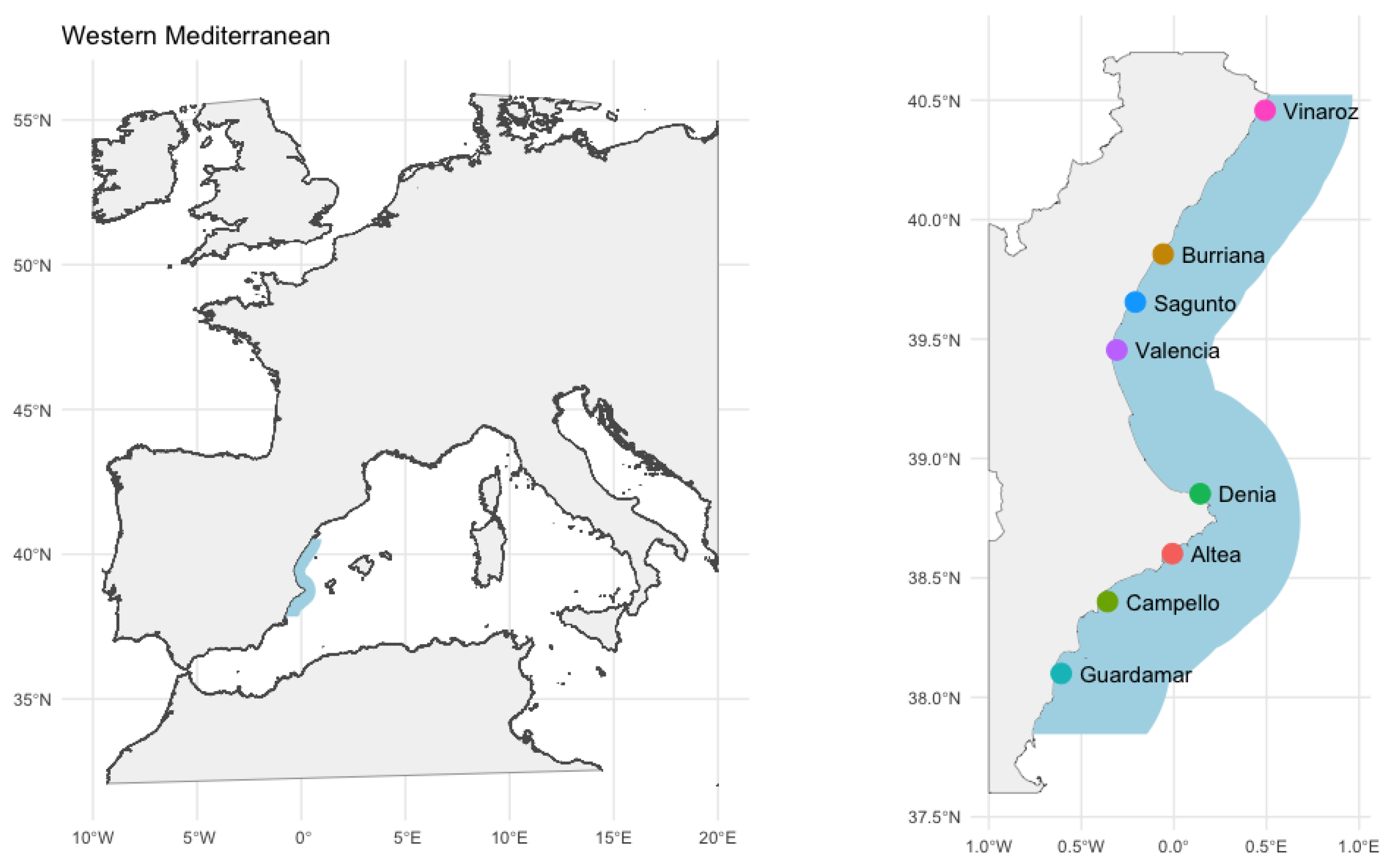
Figure 2.
Seasonal time series of SST at each location, showing observed data and ARIMA-based 10-year prediction band (pink). The shaded area indicates the forecast uncertainty. The plot highlights seasonal variation, with summer months showing higher inter-annual variability, while winter months remain relatively stable.
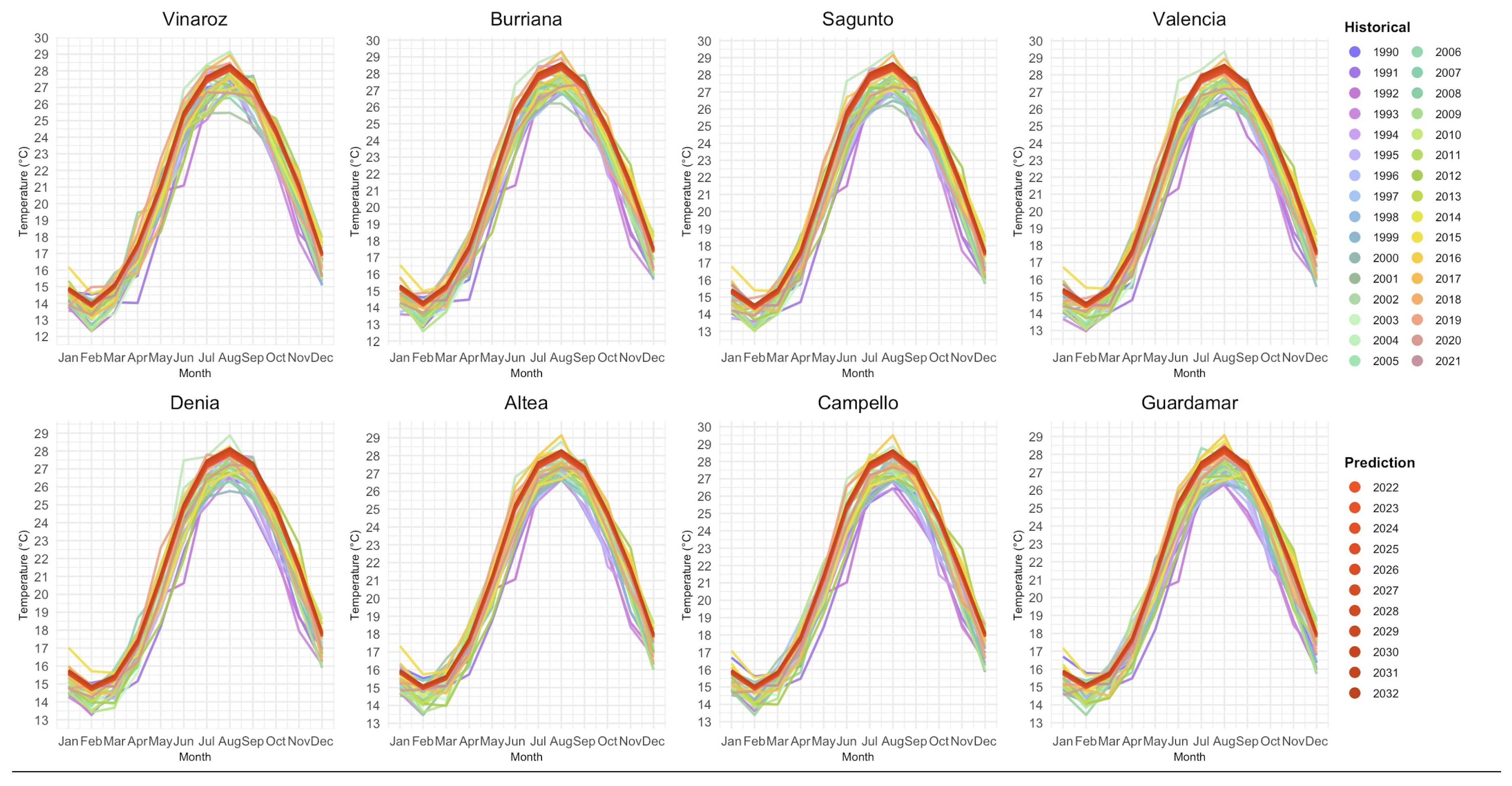
Figure 3.
Trend decomposition of SST time series and 10-year ARIMA predictions for each location. Points represent monthly SST observations, lines the trend component, and the shaded area the prediction interval. Seasonal and latitudinal variations are captured in the trend component
Figure 3.
Trend decomposition of SST time series and 10-year ARIMA predictions for each location. Points represent monthly SST observations, lines the trend component, and the shaded area the prediction interval. Seasonal and latitudinal variations are captured in the trend component
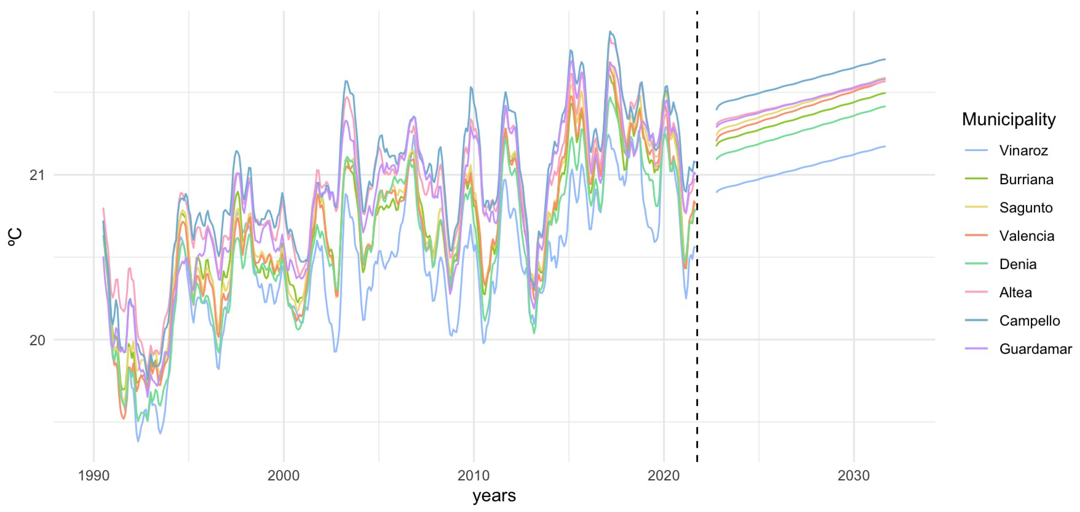
Figure 4.
Predicted maximum monthly SST (June–October) across all locations from 1995 to 2024, obtained from the spatio-temporal INLA model. Colors represent SST in °C. The model captures both spatial and temporal variation, with the shaded areas (or color gradient) reflecting the uncertainty of the predictions. A slight upward trend is observed in maximum SST, particularly during 2015–2024. The effective range of the spatial Gaussian field is 246 km, indicating the distance over which spatial correlation stabilizes.
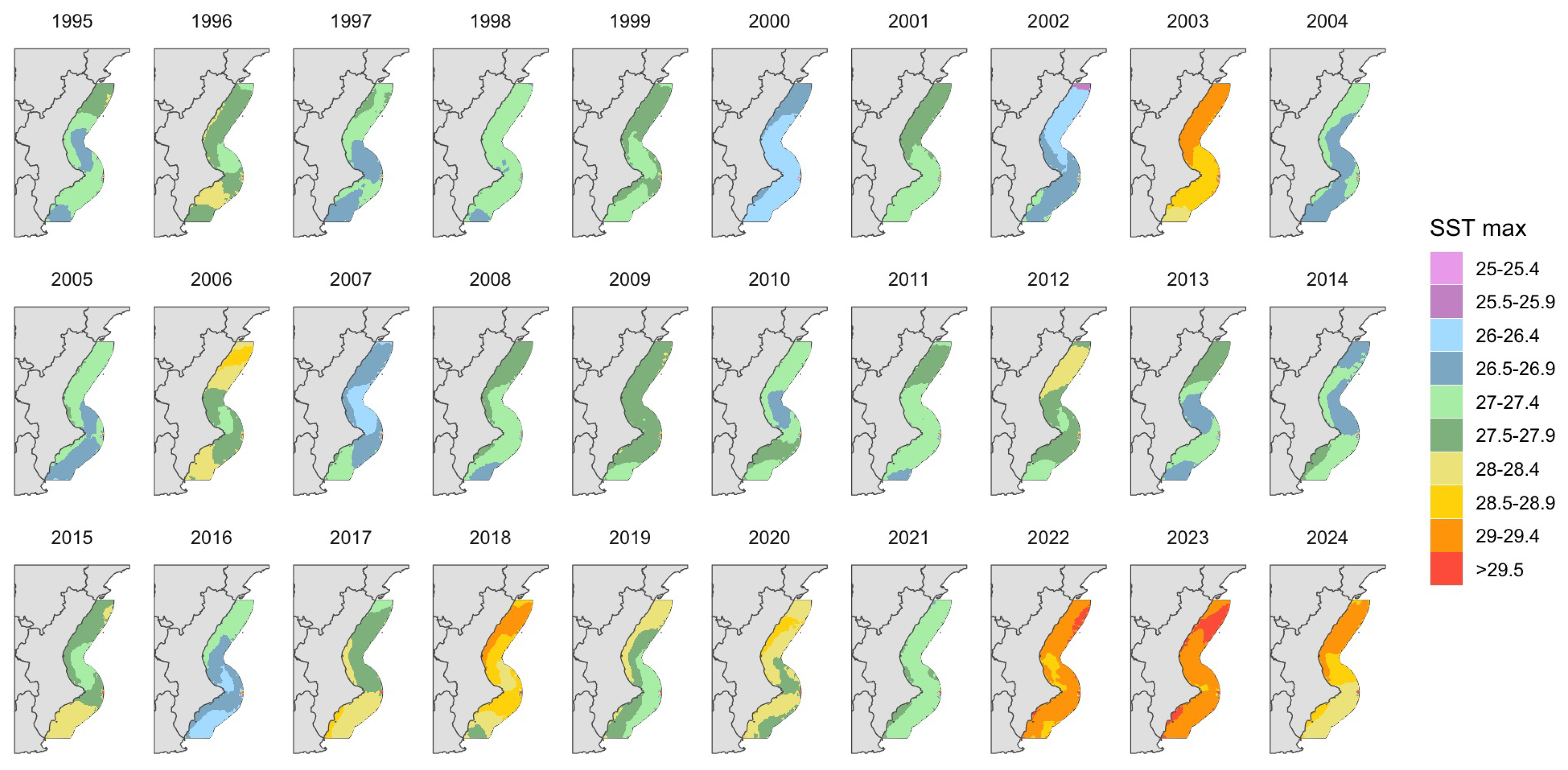
Figure 5.
Predicted range of monthly SST (difference between maximum and minimum SST) for June–October, 1995–2024. Colors indicate the magnitude of SST variability (°C), with higher ranges corresponding to greater intra-annual variation. The spatial model accounts for temporal and spatial correlation, with an effective range of 207 km.
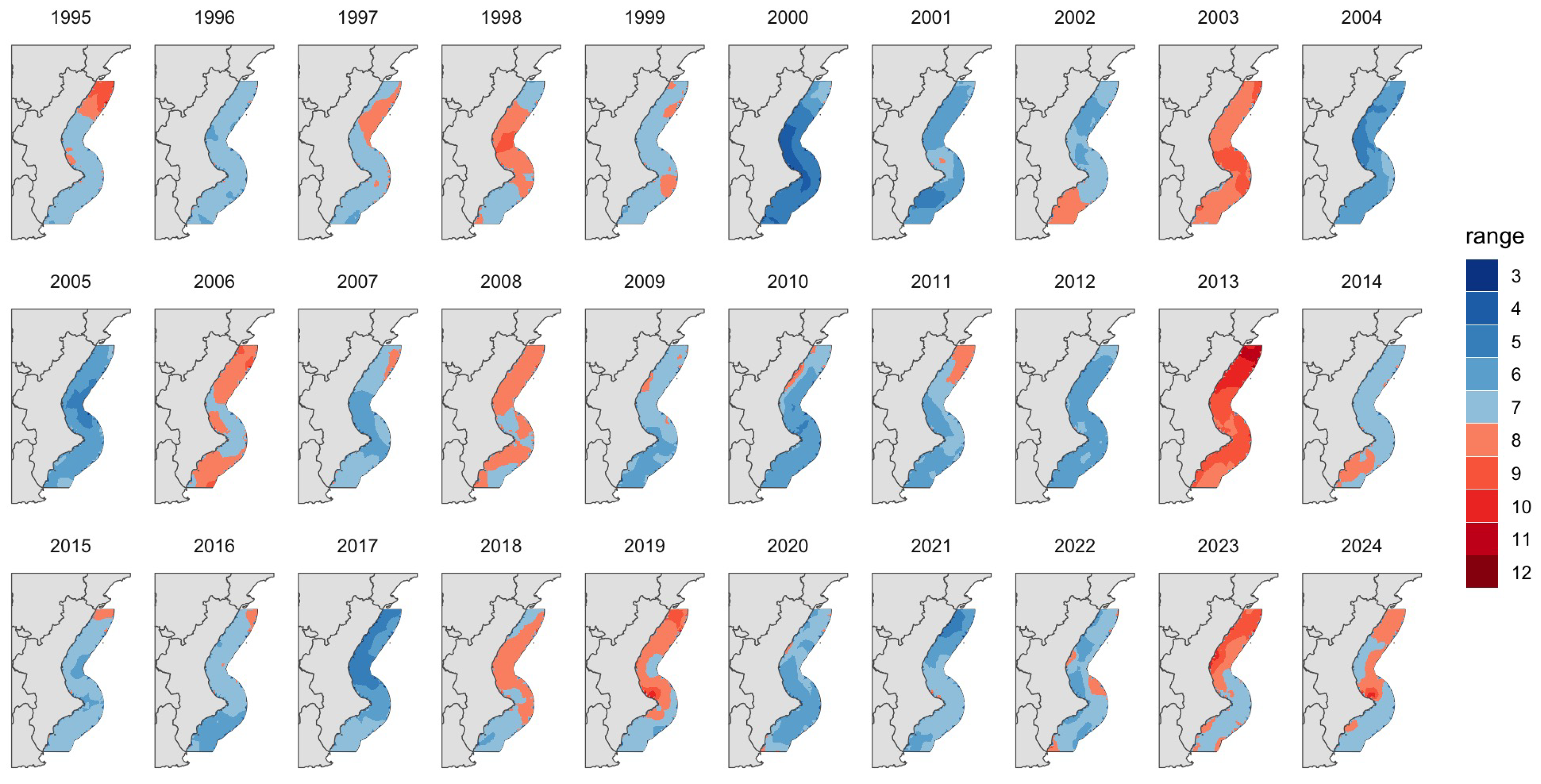
Figure 6.
Sen’s slope estimates for the long-term trends in SST maxima (panel a) and SST ranges (panel b) across the study area. The slopes quantify annual change (°C/year), highlighting areas with significant warming or increased variability. This analysis complements the spatio-temporal model predictions, confirming the seasonal and inter-annual patterns of warming and variability.
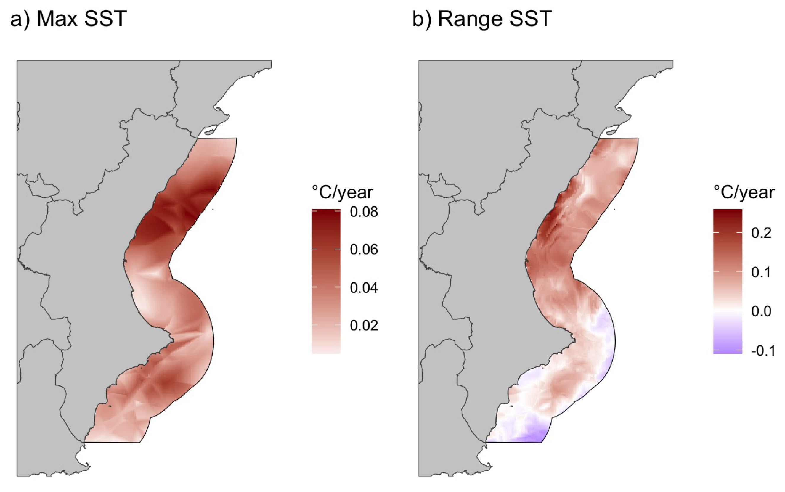
Figure 7.
Estimated smooth effects of cyclic month, AMO, ENSO index, and lagged NAO on monthly SST, obtained from the GAM. Each panel shows the partial effect of the corresponding predictor, with the solid line representing the estimated smooth function and the shaded area its 95% confidence interval (calculated using the Bayesian covariance matrix of the smooth). The y-axis indicates the deviation in SST (°C) relative to the model intercept. A smooth is considered statistically significant if its confidence band does not overlap zero and/or if the associated approximate significance test (summary output) yields .
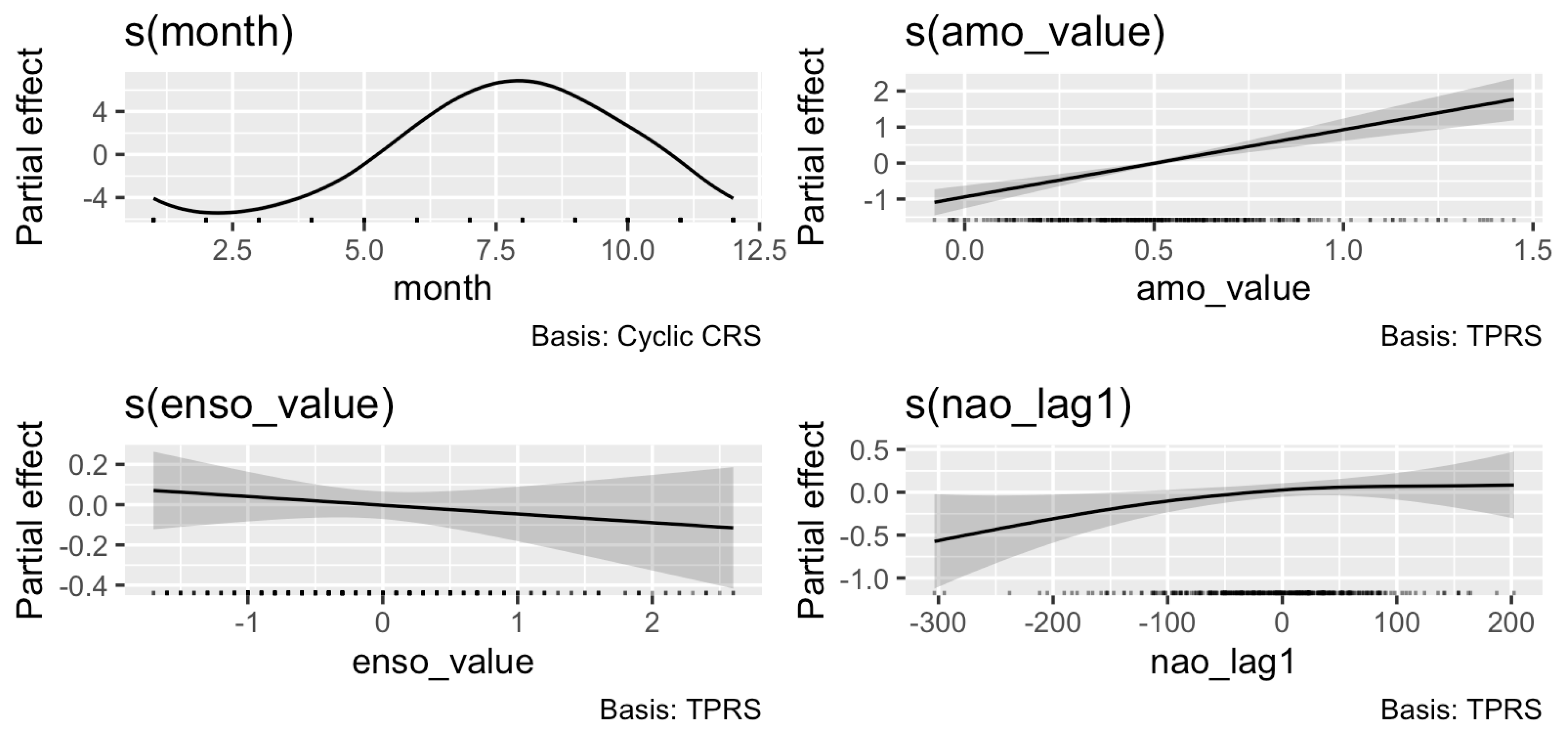
Figure 8.
Forest plot of estimated annual effects (±95% confidence intervals) of year on monthly sea surface temperature (SST), relative to the baseline year 1995. Points represent model coefficients from the GAM, with vertical lines indicating approximate 95% confidence intervals calculated as estimate ± 1.96 × SE. Years shown in red are significantly lower than the baseline ( .), based on parametric tests in the GAM summary. Non-significant effects are shown in black. The dashed horizontal line marks zero, i.e., no difference from the reference year.
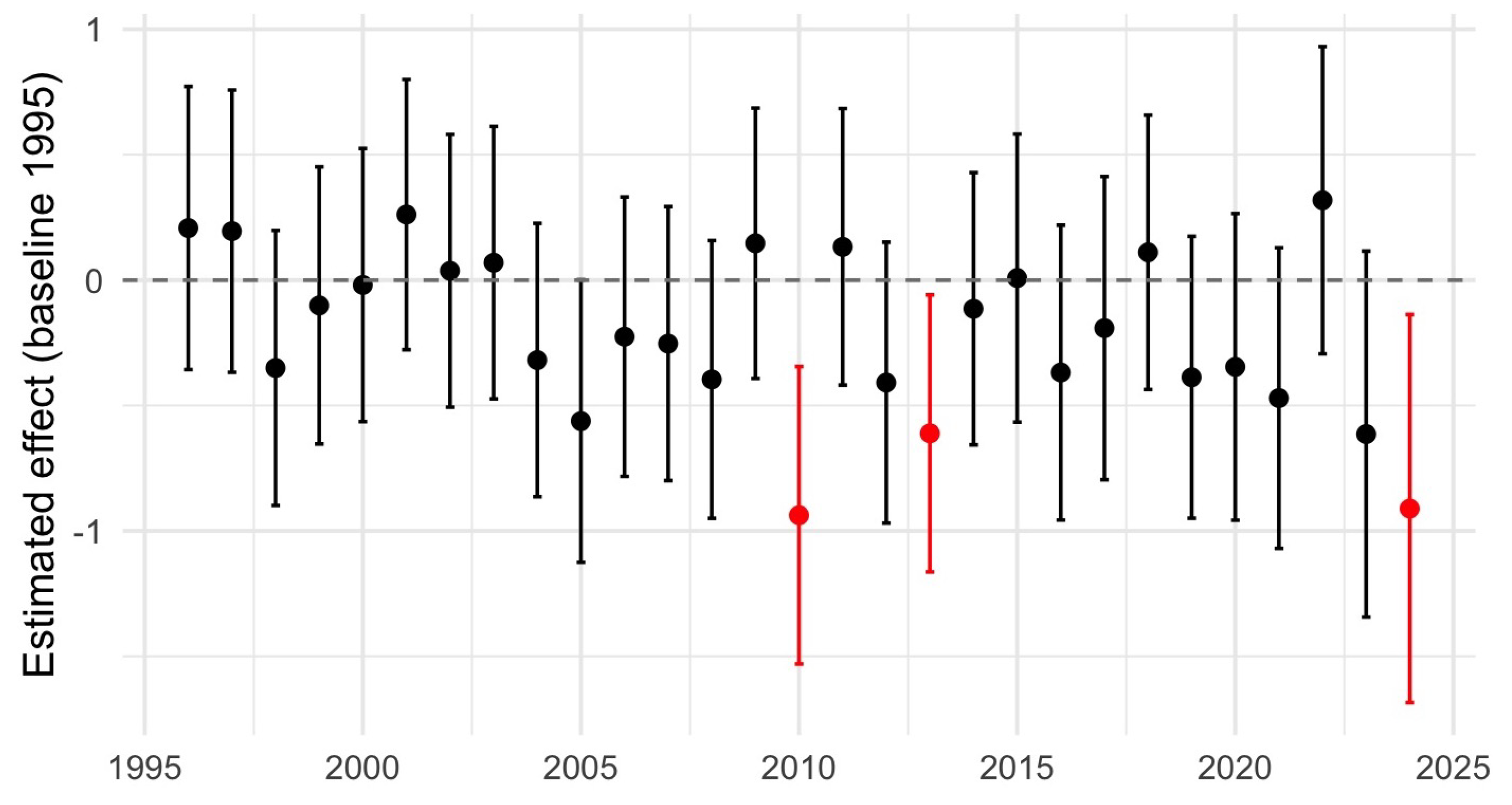
Figure 9.
Seasonal time series of SST at each location, showing observed data and ARIMA-based 10-year prediction band (pink). The shaded area indicates the forecast uncertainty. The plot highlights seasonal variation, with summer months showing higher inter-annual variability, while winter months remain relatively stable.
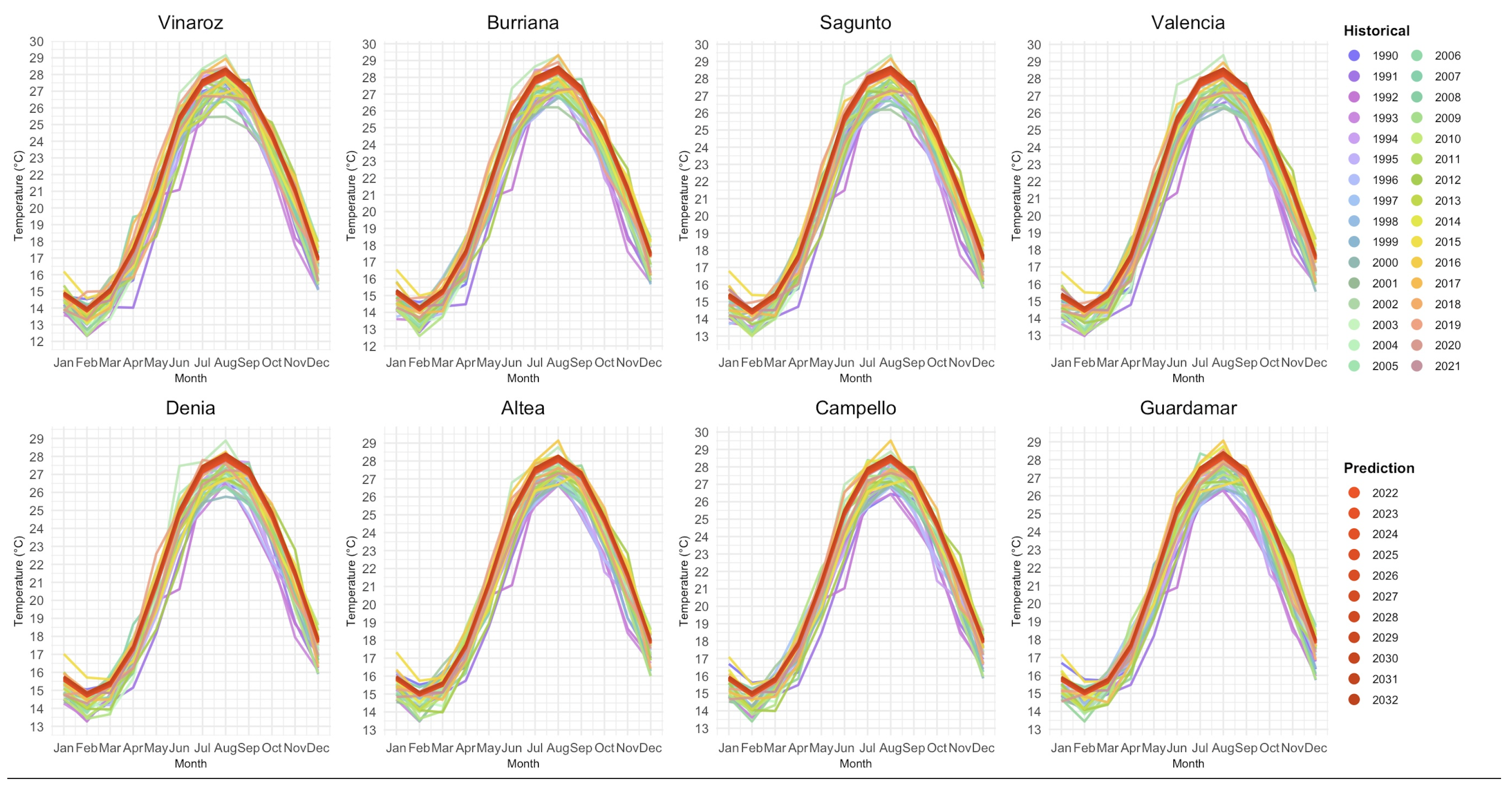
Figure 10.
Trend decomposition of SST time series and 10-year ARIMA predictions for each location. Points represent monthly SST observations, lines the trend component, and the shaded area the prediction interval. Seasonal and latitudinal variations are captured in the trend component
Figure 10.
Trend decomposition of SST time series and 10-year ARIMA predictions for each location. Points represent monthly SST observations, lines the trend component, and the shaded area the prediction interval. Seasonal and latitudinal variations are captured in the trend component

Figure 11.
Predicted maximum monthly SST (June–October) across all locations from 1995 to 2024, obtained from the spatio-temporal INLA model. Colors represent SST in °C. The model captures both spatial and temporal variation, with the shaded areas (or color gradient) reflecting the uncertainty of the predictions. A slight upward trend is observed in maximum SST, particularly during 2015–2024. The effective range of the spatial Gaussian field is 246 km, indicating the distance over which spatial correlation stabilizes.
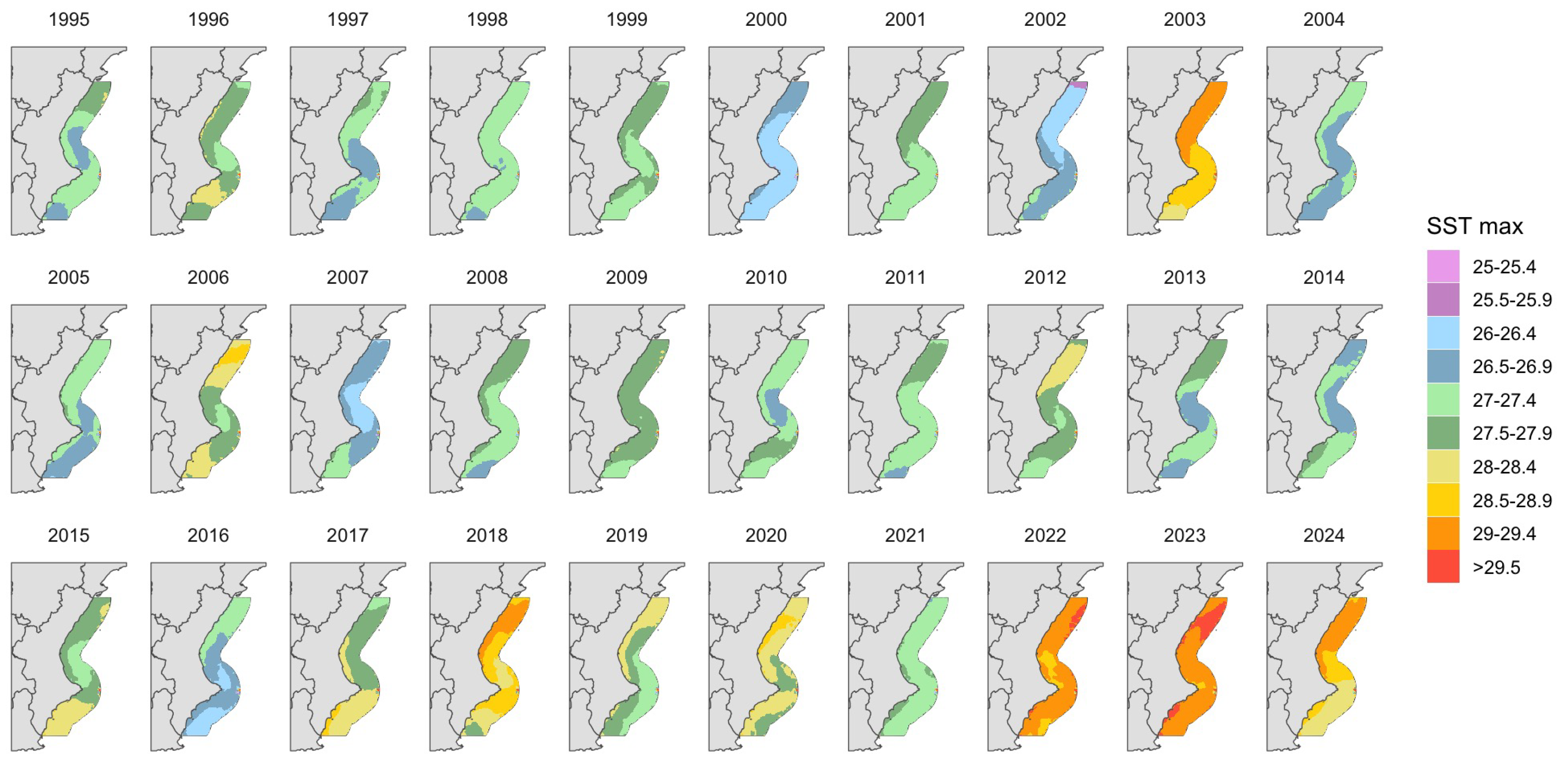
Figure 12.
Predicted range of monthly SST (difference between maximum and minimum SST) for June–October, 1995–2024. Colors indicate the magnitude of SST variability (°C), with higher ranges corresponding to greater intra-annual variation. The spatial model accounts for temporal and spatial correlation, with an effective range of 207 km.
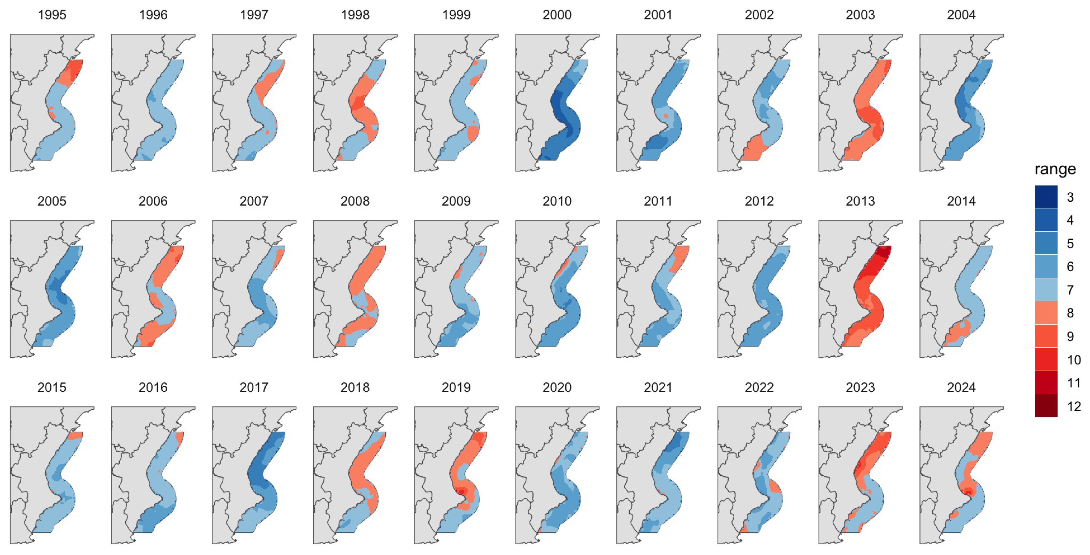
Figure 13.
Sen’s slope estimates for the long-term trends in SST maxima (panel a) and SST ranges (panel b) across the study area. The slopes quantify annual change (°C/year), highlighting areas with significant warming or increased variability. This analysis complements the spatio-temporal model predictions, confirming the seasonal and inter-annual patterns of warming and variability.
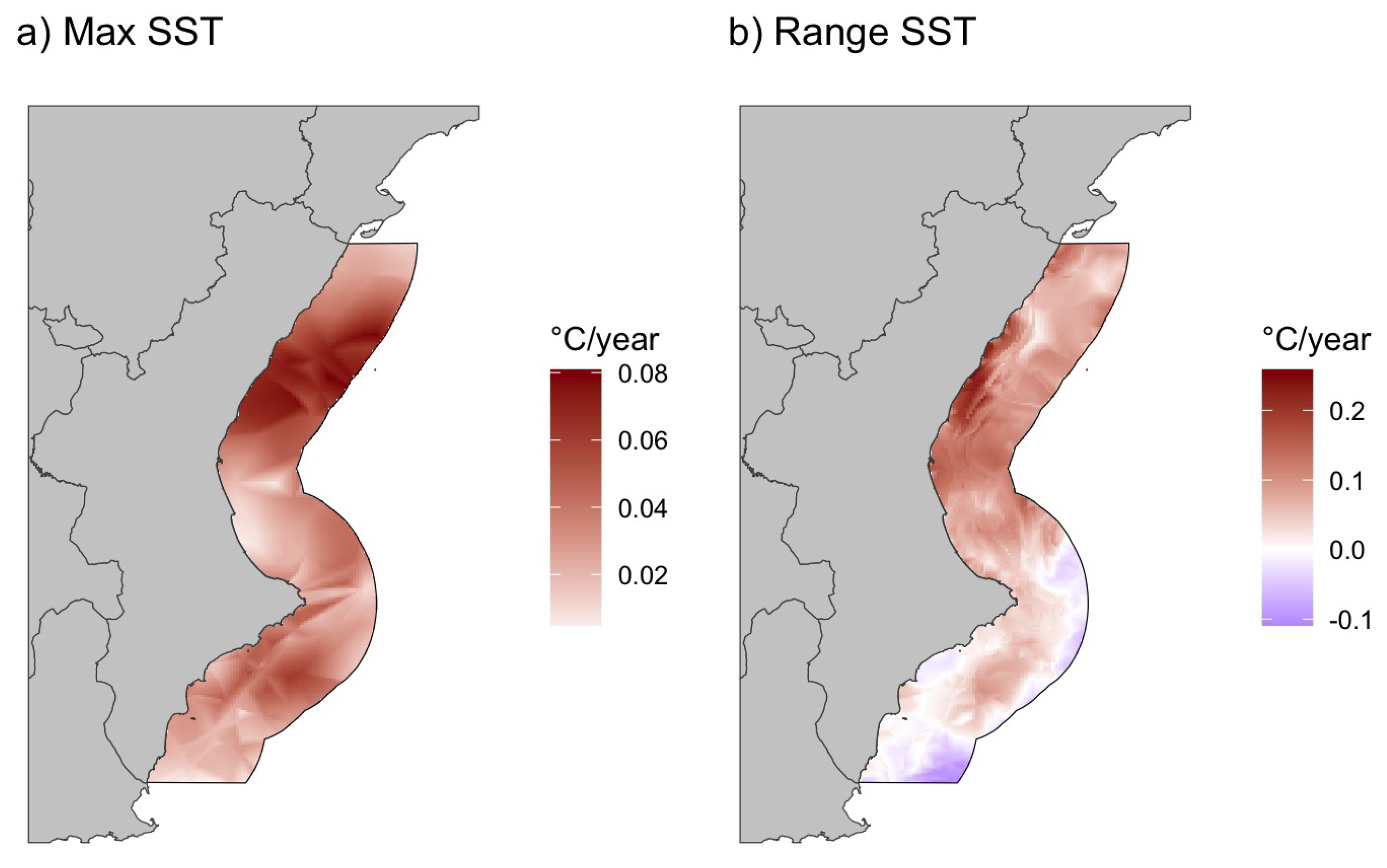
Figure 14.
Estimated smooth effects of cyclic month, AMO, ENSO index, and lagged NAO on monthly SST, obtained from the GAM. Each panel shows the partial effect of the corresponding predictor, with the solid line representing the estimated smooth function and the shaded area its 95% confidence interval (calculated using the Bayesian covariance matrix of the smooth). The y-axis indicates the deviation in SST (°C) relative to the model intercept. A smooth is considered statistically significant if its confidence band does not overlap zero and/or if the associated approximate significance test (summary output) yields .

Figure 15.
Forest plot of estimated annual effects (±95% confidence intervals) of year on monthly sea surface temperature (SST), relative to the baseline year 1995. Points represent model coefficients from the GAM, with vertical lines indicating approximate 95% confidence intervals calculated as estimate ± 1.96 × SE. Years shown in red are significantly lower than the baseline ( .), based on parametric tests in the GAM summary. Non-significant effects are shown in black. The dashed horizontal line marks zero, i.e., no difference from the reference year.
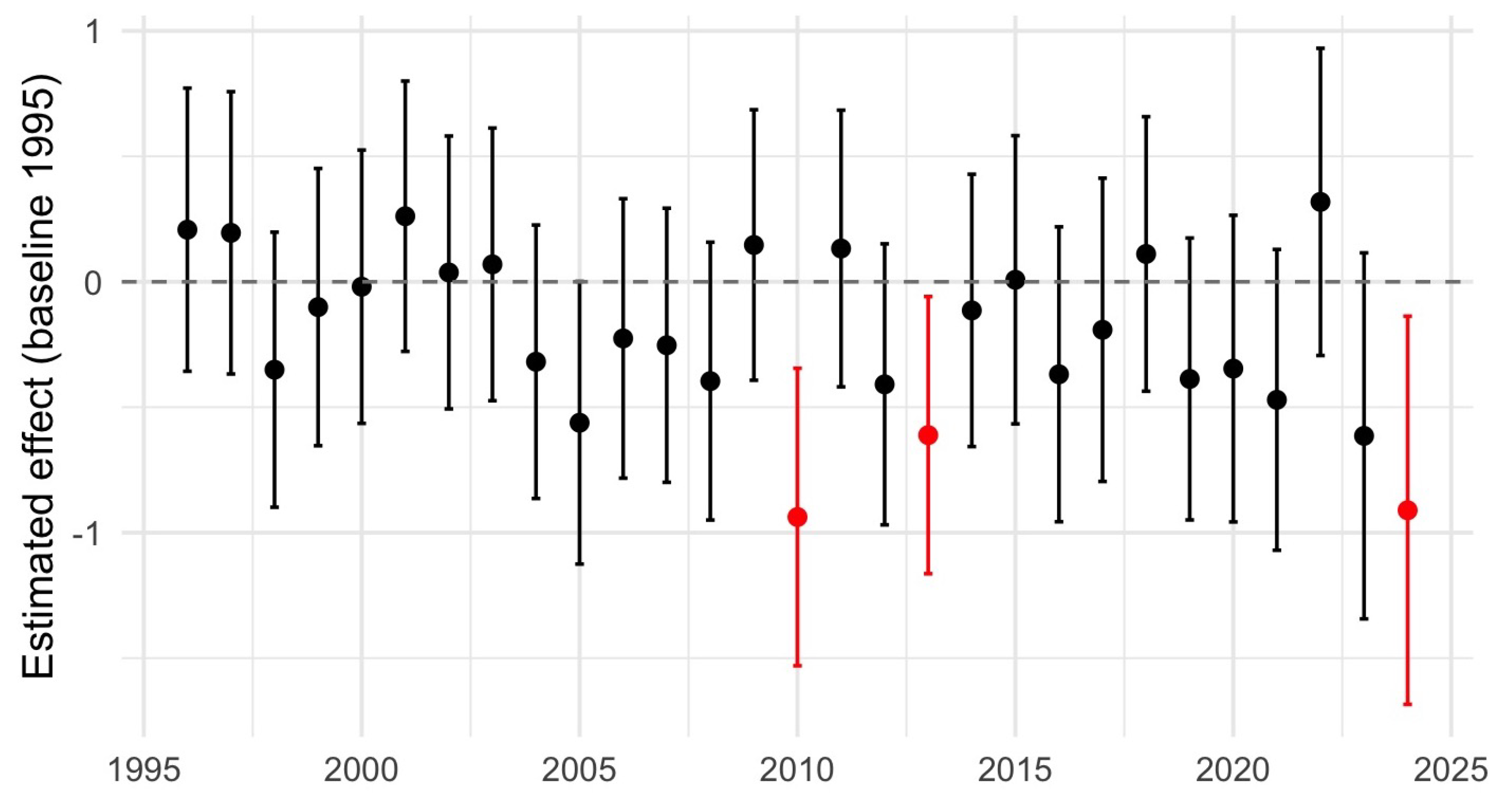

Table 1.
parameter values. represents the magnitude of the autoregressive effect from the previous month, the impact of the previous month’s error term, and the effect of the error 12 months prior. Northern locations show lower values, indicating smaller month-to-month autocorrelation, while and are similar across sites, with small differences in magnitude.
| Vinaroz | 0.300 | -1.000 | -0.922 |
| Burriana | 0.326 | -1.000 | -0.916 |
| Sagunto | 0.333 | -1.000 | -0.929 |
| Valencia | 0.350 | -1.000 | -0.930 |
| Denia | 0.387 | -1.000 | -0.920 |
| Altea | 0.404 | -1.000 | -0.885 |
| Campello | 0.416 | -0.997 | -0.925 |
| Guardamar | 0.386 | -0.994 | -0.900 |
Table 2.
Posterior summaries of the maximum SST spatio-temporal model (40% of the data). is the intercept on the log scale, is the residual standard deviation, “Range for i” indicates the effective spatial range of the Gaussian field (km), and “sd for i” the standard deviation of the spatial effect. The results show a moderate spatial correlation (246 km) and low residual uncertainty.
| mean | sd | ||||
|---|---|---|---|---|---|
| 5.706 | 0.0024 | 5.701 | 5.706 | 5.710 | |
| 0.002 | 0.000021 | 0.002 | 0.002 | 0.002 | |
| Range for i | 246.365 | 16.756 | 212.799 | 246.700 | 278.490 |
| sd for i | 0.0046 | 0.0003 | 0.0041 | 0.0046 | 0.0051 |
Table 3.
Posterior summaries of the SST range spatio-temporal model (35% of the data). The parameters are analogous to Table \ref{tab:st_param_max}. The effective spatial range is slightly smaller (207 km), indicating stronger localized spatial correlation for SST variability.
Table 3.
Posterior summaries of the SST range spatio-temporal model (35% of the data). The parameters are analogous to Table \ref{tab:st_param_max}. The effective spatial range is slightly smaller (207 km), indicating stronger localized spatial correlation for SST variability.
| mean | sd | ||||
|---|---|---|---|---|---|
| 1.293 | 0.111 | 1.074 | 1.293 | 1.512 | |
| 0.005 | 0.000085 | 0.005 | 0.005 | 0.004 | |
| Range for i | 207.767 | 7.695 | 194.379 | 207.162 | 224.596 |
| sd for i | 0.298 | 0.010 | 0.280 | 0.297 | 0.321 |
Table 4.
Bibliographic recompilation of different studies about extreme sea surface temperatures and their effects in the Mediterranean Sea
Table 4.
Bibliographic recompilation of different studies about extreme sea surface temperatures and their effects in the Mediterranean Sea
| Years of interest | Impact type | Reference |
|---|---|---|
| 2018, 2003 | MHWs with medicanes | [39] |
| 2022, 2016 | MHWs in the West Med | [40] |
| 2003, 2020 | EMS in the West Med | [41] |
| 2008-2017 | Higher SST trend in the West Med | [42] |
| 2003, 2018, 2015 | MHWs in the West Med | [43] |
| 1998, 2003, 2012, 2015, 2022 | Sumer and Autumn MHWs in the Med | [44] |
Table 5.
Summary of smooth effects from the GAM of monthly SST.The estimated degrees of freedom (edf) indicate the complexity of the smooth function(EDF corresponds to a linear effect, higher values indicate non-linear responses).F-tests are approximate significance tests for each smooth term. SST shows a strong seasonal cycle () and a significant positive association with AMO. ENSO and lagged NAO did not contribute significantly.
| Term | EDF | Ref.df | F | p-valor |
|---|---|---|---|---|
| 7.688 | 8.000 | 1527.703 | p < 0.001 | |
| 1.000 | 1.001 | 36.031 | p < 0.001 | |
| 1.000 | 1.001 | 589 | 0.443 | |
| 1.849 | 2.388 | 2.264 | 0.930 |
Table 6.
parameter values. represents the magnitude of the autoregressive effect from the previous month, the impact of the previous month’s error term, and the effect of the error 12 months prior. Northern locations show lower values, indicating smaller month-to-month autocorrelation, while and are similar across sites, with small differences in magnitude.
| Vinaroz | 0.300 | -1.000 | -0.922 |
| Burriana | 0.326 | -1.000 | -0.916 |
| Sagunto | 0.333 | -1.000 | -0.929 |
| Valencia | 0.350 | -1.000 | -0.930 |
| Denia | 0.387 | -1.000 | -0.920 |
| Altea | 0.404 | -1.000 | -0.885 |
| Campello | 0.416 | -0.997 | -0.925 |
| Guardamar | 0.386 | -0.994 | -0.900 |
Table 7.
Posterior summaries of the maximum SST spatio-temporal model (40% of the data). is the intercept on the log scale, is the residual standard deviation, “Range for i” indicates the effective spatial range of the Gaussian field (km), and “sd for i” the standard deviation of the spatial effect. The results show a moderate spatial correlation (246 km) and low residual uncertainty.
| mean | sd | ||||
|---|---|---|---|---|---|
| 5.706 | 0.0024 | 5.701 | 5.706 | 5.710 | |
| 0.002 | 0.000021 | 0.002 | 0.002 | 0.002 | |
| Range for i | 246.365 | 16.756 | 212.799 | 246.700 | 278.490 |
| sd for i | 0.0046 | 0.0003 | 0.0041 | 0.0046 | 0.0051 |
Table 8.
Posterior summaries of the SST range spatio-temporal model (35% of the data). The parameters are analogous to Table \ref{tab:st_param_max}. The effective spatial range is slightly smaller (207 km), indicating stronger localized spatial correlation for SST variability.
Table 8.
Posterior summaries of the SST range spatio-temporal model (35% of the data). The parameters are analogous to Table \ref{tab:st_param_max}. The effective spatial range is slightly smaller (207 km), indicating stronger localized spatial correlation for SST variability.
| mean | sd | ||||
|---|---|---|---|---|---|
| 1.293 | 0.111 | 1.074 | 1.293 | 1.512 | |
| 0.005 | 0.000085 | 0.005 | 0.005 | 0.004 | |
| Range for i | 207.767 | 7.695 | 194.379 | 207.162 | 224.596 |
| sd for i | 0.298 | 0.010 | 0.280 | 0.297 | 0.321 |
Table 9.
Bibliographic recompilation of different studies about extreme sea surface temperatures and their effects in the Mediterranean Sea
Table 9.
Bibliographic recompilation of different studies about extreme sea surface temperatures and their effects in the Mediterranean Sea
| Years of interest | Impact type | Reference |
|---|---|---|
| 2018, 2003 | MHWs with medicanes | [39] |
| 2022, 2016 | MHWs in the West Med | [40] |
| 2003, 2020 | EMS in the West Med | [41] |
| 2008-2017 | Higher SST trend in the West Med | [42] |
| 2003, 2018, 2015 | MHWs in the West Med | [43] |
| 1998, 2003, 2012, 2015, 2022 | Sumer and Autumn MHWs in the Med | [44] |
Table 10.
Summary of smooth effects from the GAM of monthly SST.The estimated degrees of freedom (edf) indicate the complexity of the smooth function(EDF corresponds to a linear effect, higher values indicate non-linear responses).F-tests are approximate significance tests for each smooth term. SST shows a strong seasonal cycle () and a significant positive association with AMO. ENSO and lagged NAO did not contribute significantly.
| Term | EDF | Ref.df | F | p-valor |
|---|---|---|---|---|
| 7.688 | 8.000 | 1527.703 | p < 0.001 | |
| 1.000 | 1.001 | 36.031 | p < 0.001 | |
| 1.000 | 1.001 | 589 | 0.443 | |
| 1.849 | 2.388 | 2.264 | 0.930 |
Disclaimer/Publisher’s Note: The statements, opinions and data contained in all publications are solely those of the individual author(s) and contributor(s) and not of MDPI and/or the editor(s). MDPI and/or the editor(s) disclaim responsibility for any injury to people or property resulting from any ideas, methods, instructions or products referred to in the content. |
© 2025 by the authors. Licensee MDPI, Basel, Switzerland. This article is an open access article distributed under the terms and conditions of the Creative Commons Attribution (CC BY) license (http://creativecommons.org/licenses/by/4.0/).
Copyright: This open access article is published under a Creative Commons CC BY 4.0 license, which permit the free download, distribution, and reuse, provided that the author and preprint are cited in any reuse.


