A Non--Markovian Search for Cosmic Homeostasis: Finite Memory Detection in Galaxy Evolution from IllustrisTNG

1. Introduction

Galaxy evolution is commonly modeled as a history-dependent process that becomes effectively Markovian when conditioned on a sufficiently rich present-day state (stellar mass, halo mass, environment). In this view, past configurations matter only insofar as they shaped the current state, and deviations from population relations are treated as transient fluctuations [1,2,3].

An alternative possibility is regulated evolution, where internal structure encodes predictive information beyond instantaneous macroscopic variables. In complex systems, regulation does not imply stasis but bounded behavior enforced by feedback and memory. For galaxies, this could manifest as: (1) bounded metallicity scatter despite varying accretion histories, (2) characteristic recovery times after perturbations correlated with pre-perturbation structure, or (3) preferred states in phase space that systems tend to return to.

The central methodological challenge is that stellar mass dominates correlations and can induce apparent relationships between quantities sharing mass dependence. A credible search therefore requires explicit controls and time-directional tests rather than reliance on correlations.

This paper presents a falsification-oriented analysis testing whether non-Markovian predictive information survives once a minimal instantaneous state is accounted for, and it identifies the timescale of any such persistence. Two observables are defined from IllustrisTNG: a chemical disorder proxy ${\Xi }_{\mathrm{AMR}}$ and a recent relaxation score R. The analysis proceeds through fixed stages: raw association, mass entanglement diagnostics, mass-controlled residual association, and time-directional conditional mutual information across two lags.

2. Methods

2.1. Simulation Data

All analyses use the public IllustrisTNG cosmological simulation suite, specifically TNG100-1 at $z=0$ (snapshot 99) [1,2,3]. For each subhalo, the following are extracted:

• Local cutout HDF5 stellar particle data (metallicity, formation time, mass weights),
• SubLink merger trees for stellar mass and SFR tracks along the main progenitor branch [4].

No selection is applied on morphology, environment, or star-forming state beyond data availability and pipeline validity. Sample sizes are reported at each stage.

2.2. Chemical Memory Proxy: Age–Metallicity Disorder ${\Xi }_{\mathrm{AMR}}$

Internal chemical disorder is quantified using the dimensionless statistic

$${\Xi }_{\mathrm{AMR}}={\displaystyle \frac{{\Sigma }_{\mathrm{AMR}}}{|{\widehat{\beta }}_1|}},$$

(1)

where ${\widehat{\beta }}_1$ is the weighted least-squares slope of ${log}_{10}\left(Z\right)$ against an age proxy ${\tau }_i=-ln\left(a_i\right)$, and ${\Sigma }_{\mathrm{AMR}}$ is the mean within-age-bin metallicity scatter (Appendix A.1). The normalization suppresses trivial scale effects, making ${\Xi }_{\mathrm{AMR}}$ interpretable as scatter per unit enrichment trend.

2.3. Recent Relaxation Score R

Recent relaxation is measured using deviations from the star-forming main sequence (SFMS) [5,6]. For fitted SFMS parameters $(a,b)$,

$$D\left(t\right)=\left|{log}_{10}\mathrm{SFR}\left(t\right)-\left[a({log}_{10}{M}_{★}\left(t\right)-10.5)+b\right]\right|,$$

(2)

computed over the recent window $[t_0-4\mathrm{Gyr},t_0]$. The 4 Gyr window captures approximately two to three galactic dynamical times for Milky Way-mass systems [7], sufficient to observe recovery from typical perturbations while remaining computationally tractable. The relaxation score $R\in [0,1]$ is a bounded transform of late deviation $D_{\mathrm{late}}$ and recovery trend $D_{\mathrm{slope}}$ (Appendix A.2). Larger R indicates closer alignment with SFMS or recovery toward it.

2.4. Test Sequence and Decision Rules

The analysis follows a fixed test sequence:

• T1 (Raw association): Pearson r and Spearman $\rho$ for $({\Xi }_{\mathrm{AMR}},R)$.
• T2 (Mass entanglement): Correlations of $m={log}_{10}{M}_{★}$ with ${\Xi }_{\mathrm{AMR}}$ and R.
• T3 (Mass-controlled association): Linear residualization against m, then correlation of residuals.
• T4 (Decomposition): Associations with components $D_{\mathrm{late}}$ and $D_{\mathrm{slope}}$.
• T5 (Time-directional test): Bias-corrected k-nearest neighbor conditional mutual information with conditional permutation nulls.

A practical-zero detectability floor is fixed at $ϵ=0.01$ bits. Full falsification logic is in Appendix B.

2.5. Non-Markovian Probe: kNN Conditional Mutual Information

To test time-directional predictive information across lags, the following quantity is estimated:

$$I\left({\Xi }_{\mathrm{AMR}}\left(t_i\right);R\left(t_0\right)\mid M_{★}\left(t_i\right)\right)$$

(3)

using a kNN conditional mutual information estimator (Frenzel-Pompe) under $L_{\infty }$ metric [8,9].

Finite-sample bias is addressed via conditional permutation:

$$I_{\mathrm{corr}}\equiv I_{\mathrm{obs}}-\mathrm{median}\left(I_{\mathrm{perm}}\right),$$

(4)

where $I_{\mathrm{perm}}$ results from permuting ${\Xi }_{\mathrm{AMR}}\left(t_i\right)$within quantile bins of $M_{★}\left(t_i\right)$, preserving the $\Xi$–mass relation while destroying conditional linkage to $R\left(t_0\right)$. The permutation p-value is $Pr(I_{\mathrm{perm}}\ge I_{\mathrm{obs}})$, with robustness evaluated across $k\in \{3,5,7,10\}$.

3. Results

3.1. Sample Construction

Two datasets are used:

• Pilot mass-matched sample ($N=8$): Pipeline validation.
• Full merged sample ($N=88$): All subhalos with successful cutouts and valid relaxation tracks, merged on subhalo_id.

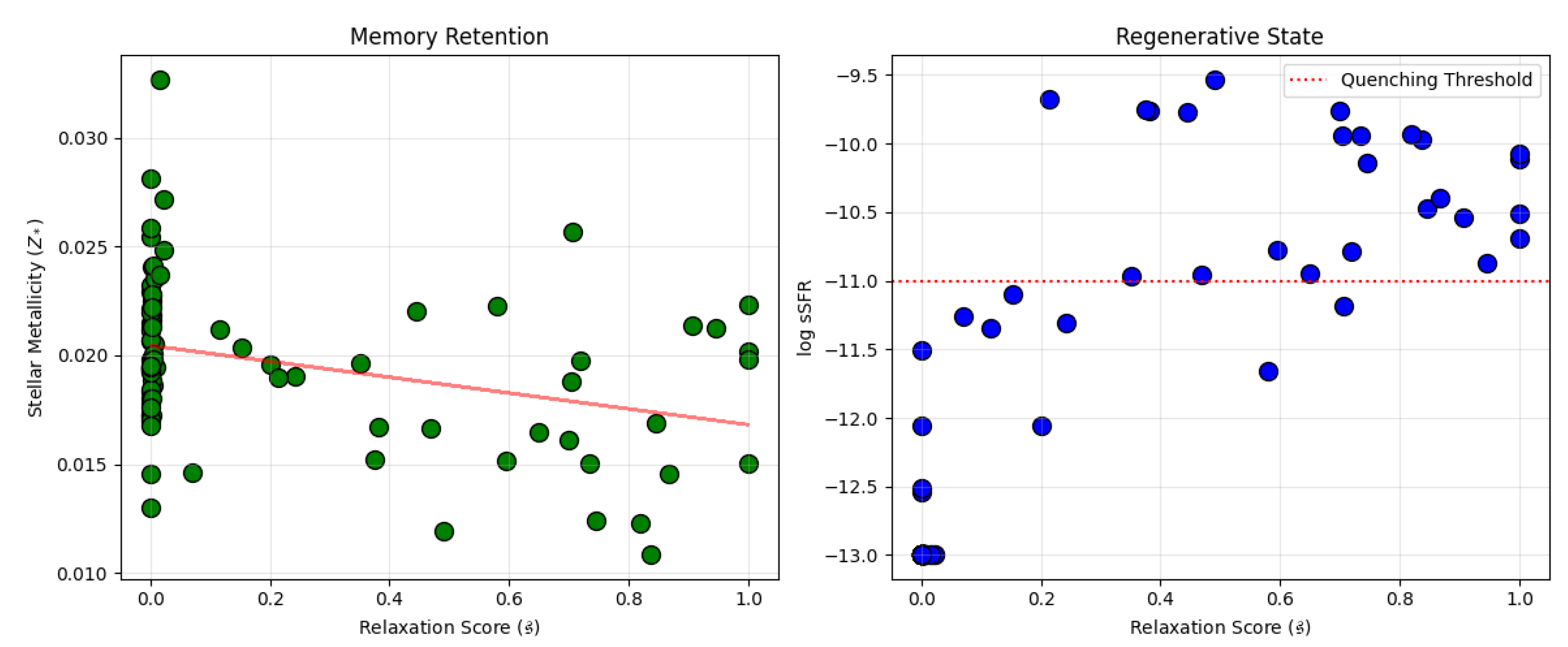
3.2. Raw Association Is Weak (T1)

In the full sample, raw association between ${\Xi }_{\mathrm{AMR}}$ and R is weak:

$$r\simeq 0.148(p\simeq 0.168),\rho \simeq 0.115(p\simeq 0.287),$$

(5)

with bootstrap confidence intervals including zero [10].

3.3. Mass Entanglement Is Significant (T2)

Mass diagnostics show entanglement:

$$\begin{array}{cc}\hfill \mathrm{corr}(m,{\Xi }_{\mathrm{AMR}})& \simeq 0.430(p\simeq 2.86\times {10}^{-5}),\hfill \end{array}$$

(6)

$$\begin{array}{cc}\hfill \mathrm{corr}(m,R)& \simeq -0.231(p\simeq 0.0306),\hfill \end{array}$$

(7)

where $m={log}_{10}{M}_{★}$.

3.4. Association Emerges After Mass Control (T3)

After linear residualization against m:

$$r_{\mathrm{resid}}\simeq 0.282,{\rho }_{\mathrm{resid}}\simeq 0.219.$$

(8)

This motivates time-directional testing, as T3 alone is not a memory test.

3.5. Relaxation Component Diagnostics (T4)

Component checks using $(D_{\mathrm{late}},D_{\mathrm{slope}})$ do not isolate a single dominant driver. The relaxation score encodes a blend of offset magnitude and recovery trend [5,6].

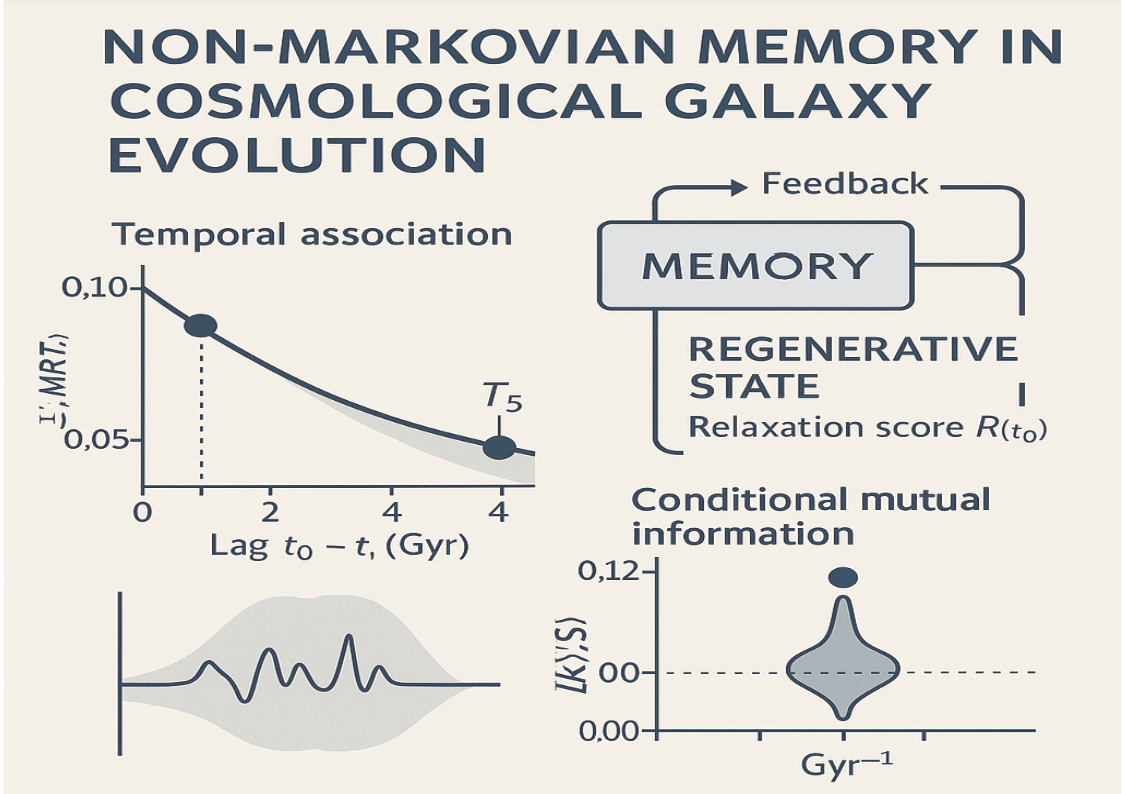
3.6. Temporal Predictive Information and Lag-Level Falsification (T5)

The temporal probe uses $X={\Xi }_{\mathrm{AMR}}\left(t_i\right)$, $Y=R\left(t_0\right)$, conditioning on $M_{★}\left(t_i\right)$ with bias-corrected kNN CMI under conditional permutation nulls.

3.6.0.1. Lag $\Delta t=2$ Gyr.

$${\widehat{I}}_{\mathrm{corr}}\left(2\mathrm{Gyr}\right)\approx 0.05875\mathrm{bits},p_{\mathrm{perm},\mathrm{med}}\approx 0.00833.$$

(9)

This lag is not falsified under the registered rule. Lag $\Delta t=4$ Gyr.

$${\widehat{I}}_{\mathrm{corr}}\left(4\mathrm{Gyr}\right)\approx 0.00050\mathrm{bits},p_{\mathrm{perm},\mathrm{med}}\approx 0.41917,$$

(10)

satisfying lag-level falsification under $ϵ=0.01$ bits.

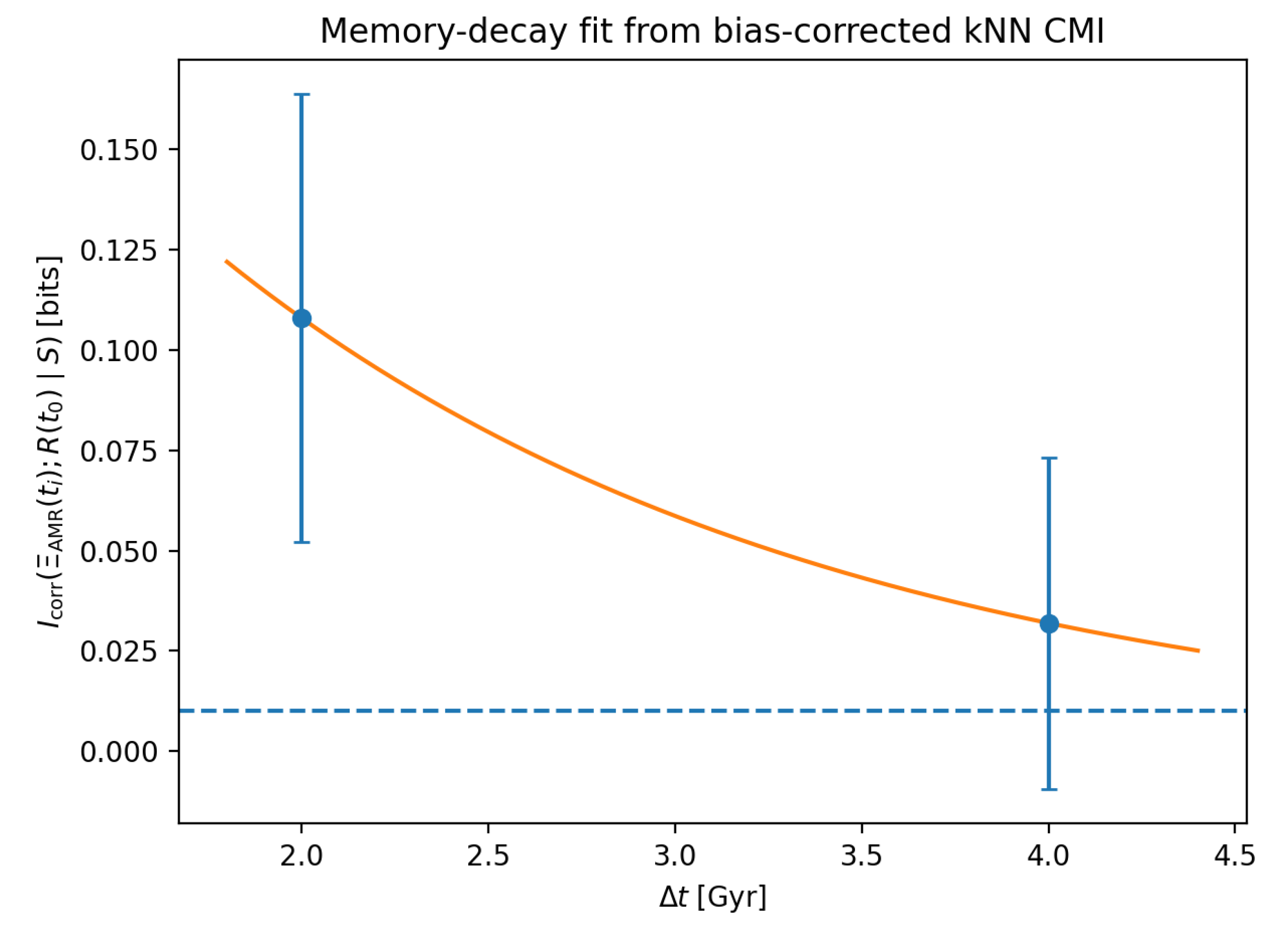
Interpretation of decay curve.

A decay visualization was produced (Fig. Figure 6) by fitting $I_{\mathrm{corr}}\left(\Delta t\right)=I_{\infty }+I_{0}exp(-\Delta t/\tau )$ to the lag-wise robust statistic. With only two distinct lag points, the fitted parameters are underdetermined; therefore $\tau$ is treated as descriptive, not inferential. Formal estimation requires denser lag sampling.

3.6.0.4. Status of the decay timescale estimate.

At the present stage, the decay model

$$I_{\mathrm{corr}}\left(\Delta t\right)=I_{\infty }+I_{0}exp(-\Delta t/\tau )$$

(11)

is included for descriptive visualization only. With only two distinct lag points ($\Delta t=2$ and $4\mathrm{Gyr}$), the parameter $\tau$ is not statistically identifiable and should not be interpreted as an inferred physical timescale. Any fitted value merely summarizes the observed short–lag decay trend and serves as a placeholder for future densely sampled lag scans. A meaningful estimation of $\tau$ requires at least three, and preferably more, independent lag points spanning the transition from detectable to negligible conditional predictive information, as outlined in Appendix C.

Figure Index and Test Mapping

Table 1 lists the principal figures used in this version of the paper, the scripts that generate them, and the registered test each figure informs. This table is included to prevent selective interpretation and to make the empirical program auditable end–to–end.

4. Figures and Interpretation (Current Best Set)

This section consolidates the most informative figures produced by the current pipeline. All files are referenced by their exact simulation output names. Interpretations are written to match the program logic: descriptive plots are not treated as evidence of non–Markovianity unless they survive explicit controls and time-directional tests.

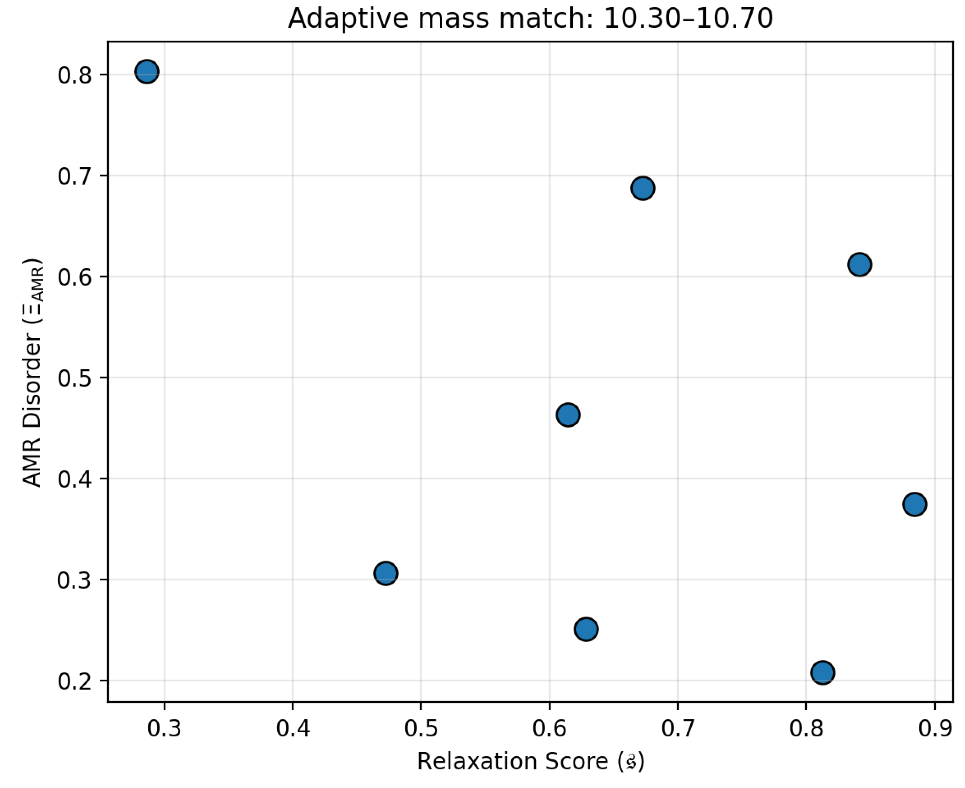
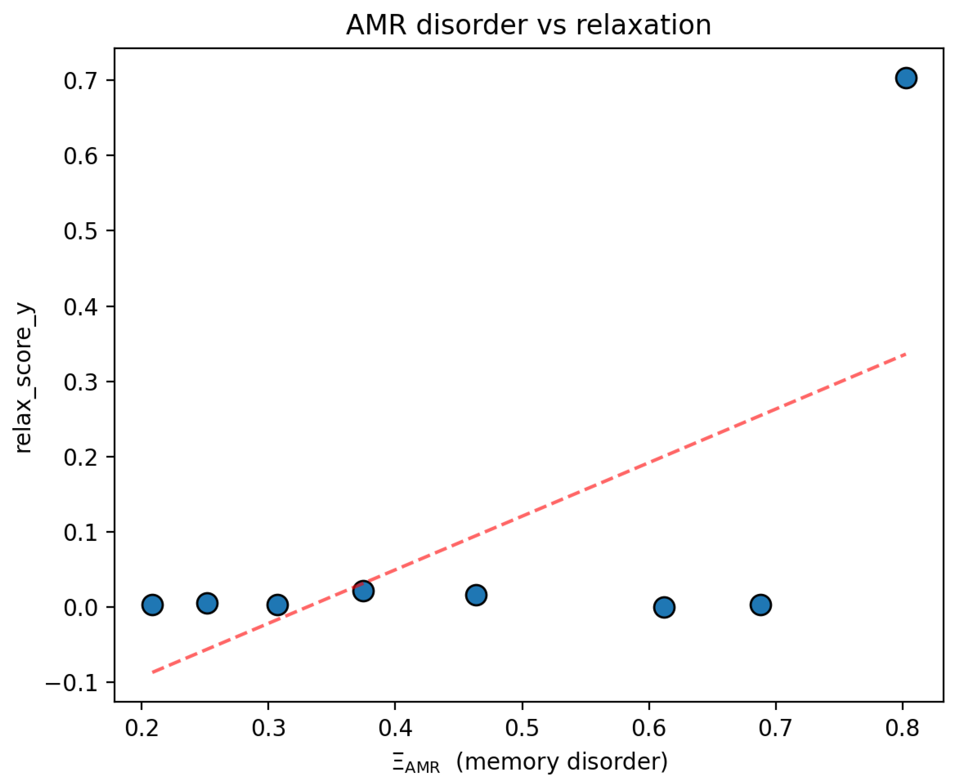
4.1. Pipeline Sanity and Pilot Context (Mass-Matched)

Interpretation. This pilot is not used for inference. Its role is diagnostic: it verifies that ${\Xi }_{\mathrm{AMR}}$ varies non-degenerately at small N and that the cutout-based measurement does not collapse to a constant under mass-matching. Any apparent trend here is treated as unstable by design because N is small. The pilot exists to prevent mistaking a broken metric for a null scientific result.

Interpretation. This figure checks whether the two quantities can be merged and visualized without pathological behaviour (e.g. constant R, constant $\Xi$, obvious data-entry errors). No claim is extracted. At best, it motivates scaling up to the full sample where mass structure is allowed to exist and must be explicitly controlled.

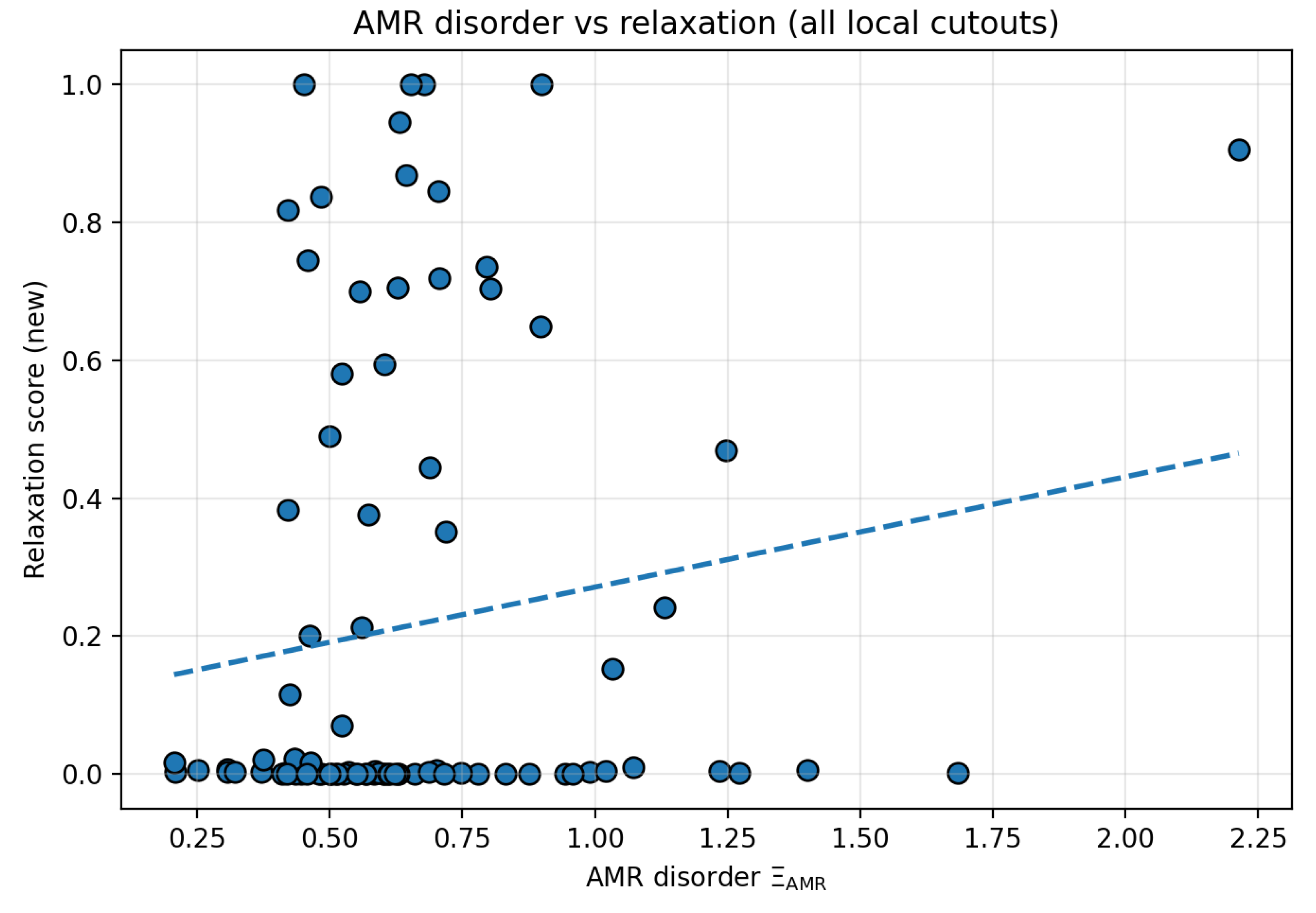
4.2. Full-Sample Structure and the Mass Dominance Problem

Interpretation. The main message is methodological. In raw space, ${\Xi }_{\mathrm{AMR}}$ and R do not show a strong monotonic relationship. However, the accompanying mass diagnostics demonstrate that mass is a structural organizer: it correlates strongly with ${\Xi }_{\mathrm{AMR}}$ and also correlates (more weakly) with R. A naïve $\Xi$–R correlation can therefore be masked, induced, or sign-flipped by shared dependence on mass. For that reason, full-sample raw correlation plots are treated as descriptive only, motivating mass control and time-directional testing.

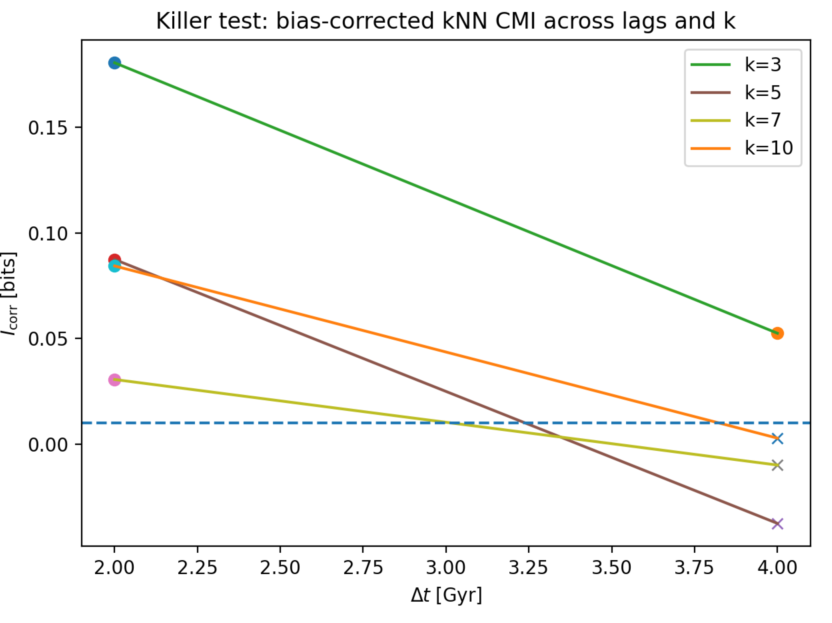
4.3. Time-Directional Falsification: The Killer CMI Test

Interpretation. This is the first plot in the paper that is capable, by construction, of supporting a non–Markovian claim under the program definition. It is time-directional (past → future) and conditioned so that the null preserves Markovian structure via mass. At $\Delta t=2$ Gyr, the bias-corrected conditional predictive information is detectable under multiple k values with small permutation p-values, indicating that earlier-time chemical disorder retains predictive information about present-day relaxation beyond mass-at-time. At $\Delta t=4$ Gyr, the signal collapses to practical zero and is not statistically distinguishable from the conditional null across the tested k values. Under the registered rules, that lag is marked falsified while the short lag is not, so the program continues. The current picture is short-horizon predictive memory rather than long persistence.

4.4. Lag-Aggregated Memory Points (v2 Scan Summary)

Interpretation. This figure summarizes the lag dependence in the most compact form the pipeline can support at the current stage. With only two lags executed (2 and 4 Gyr), the correct interpretation is qualitative: predictive information is visible at 2 Gyr and absent at 4 Gyr under the present conditioning. A meaningful estimate of a decay timescale $\tau$ requires at least three distinct lags; until then, any fitted curve is treated as descriptive, not inferential. The next phase is therefore a denser lag scan (e.g. 1–6 Gyr) combined with an expanded conditioning vector to test whether the apparent horizon is a real decay or a confounding artifact.

4.5. What These Figures Jointly Imply (Without Overclaiming)

Joint reading.Figure 4, Figure 5 and Figure 6 jointly support a narrow, auditable interim statement. Raw association is weak because mass entanglement dominates. Once a time-directional test is enforced with a conditional null that preserves the $\Xi$–mass relationship, conditional predictive information is detected at short lag and not at longer lag. This pattern is consistent with a bounded memory horizon in this observable family, under this simulation and this minimal conditioning set. The program therefore continues, but it is already constrained: “homeostasis” does not appear as long-lived predictive information in ${\Xi }_{\mathrm{AMR}}$ beyond 4 Gyr under mass-at-time conditioning.

5. Discussion

5.0.0.5. Numerical and Subgrid Limitations

All results reported here are subject to the finite resolution and subgrid physics of the TNG100–1 simulation. The baryonic mass resolution ($m_{\mathrm{bar}}\sim 1.4\times {10}^6{M}_{\odot }$) implies that stellar populations and metallicity distributions are sampled discretely, which can introduce artificial smoothing or stochasticity into age–metallicity relations. In addition, feedback and star formation subgrid models operate on timescales significantly shorter than the ∼Gyr memory horizon probed here, potentially imprinting correlated structure that mimics or masks true long–term regulation. These limitations do not invalidate the conditional tests performed, but they do caution against over–interpreting the detected short–lag signal as a direct analogue of physical memory without cross–validation in higher–resolution runs or alternative simulation suites.

5.1. Summary of Findings

The results support three concrete statements:

(1) Mass dominance is nontrivial.

Raw correlations between chemical disorder and relaxation are not interpretable without controls, as stellar mass is entangled with both observables.

(2) A non-mass linkage exists at residual level.

Moderate association after mass residualization indicates that ${\Xi }_{\mathrm{AMR}}$ and R encode partially independent variation.

(3) Time-directional test indicates finite predictive horizon.

Conditional predictive information is detectable at $\Delta t\approx 2$ Gyr under minimal conditioning but is consistent with zero by $\Delta t\approx 4$ Gyr. This suggests finite memory rather than indefinite predictability for this observable pair.

Table 2. Comparison of detected memory timescale to known galactic processes. The $\sim 2$ Gyr horizon aligns with gas depletion and orbital mixing timescales.

Physical Process	Typical Timescale (Gyr)	Relation to $\sim 2$ Gyr memory
Dynamical time	0.1–1	Memory $\sim 2$–$20\times {\tau }_{\mathrm{dyn}}$
Gas depletion time	1–3	Memory $\sim {\tau }_{\mathrm{dep}}$
Orbital mixing time	1–10	Memory within this range
Feedback cycle time	0.01–1	Memory $>{\tau }_{\mathrm{feedback}}$

Table 2. Comparison of detected memory timescale to known galactic processes. The $\sim 2$ Gyr horizon aligns with gas depletion and orbital mixing timescales.

Physical Process	Typical Timescale (Gyr)	Relation to $\sim 2$ Gyr memory
Dynamical time	0.1–1	Memory $\sim 2$–$20\times {\tau }_{\mathrm{dyn}}$
Gas depletion time	1–3	Memory $\sim {\tau }_{\mathrm{dep}}$
Orbital mixing time	1–10	Memory within this range
Feedback cycle time	0.01–1	Memory $>{\tau }_{\mathrm{feedback}}$

5.2. Connection to Homeostasis Concept

The detected finite predictive horizon ($\sim 2$ Gyr) suggests finite-memory regulation rather than perfect homeostasis. In complex systems, regulation often involves feedback loops with characteristic timescales; the observed memory decay may reflect the timescale of internal processes (e.g., gas cycling, feedback cycles) that gradually erase historical information. This represents a third regime between Markovian drift and perfect memory.

5.3. Statistical Power and Detectability Limits

The present analysis operates close to the minimum detectability threshold imposed by finite sample size. With $N=88$ galaxies, the bias–corrected conditional mutual information detected at $\Delta t=2\mathrm{Gyr}$ ($I_{\mathrm{corr}}\simeq 0.06$ bits) lies only modestly above the practical resolution floor of the estimator under conditional permutation ($\sim 0.05$ bits). This proximity implies that the detected signal should be interpreted as marginal but non–negligible evidence rather than a high–signal regime detection. Increased sample size, denser lag sampling, or expanded conditioning vectors are expected to improve power and sharpen discrimination between true short–memory behaviour and residual finite–sample fluctuations.

5.4. Limitations and Scope

These conclusions are deliberately narrow. The CMI configuration conditions only on $M_{★}\left(t_i\right)$. A richer instantaneous state vector may absorb part of the short-lag signal, or it may clarify whether signal persists with additional confounders controlled. Alternative memory proxies may yield different horizons.

Numerical considerations: Subgrid feedback models in TNG100 inject energy on characteristic timescales (typically $<1$ Gyr). While the detected $\sim 2$ Gyr memory exceeds typical feedback cycles, comparison with higher-resolution simulations (e.g., TNG50) could help separate physical memory from potential numerical artifacts. The finite particle resolution ($m_{\mathrm{bar}}\sim 1.4\times {10}^6$ M_⊙) sets a lower bound on detectable structural information.

5.5. Interpreting Outcomes in a Falsification Framework

In this framework, both outcomes are informative:

• Signal detection: Indicates non-Markovian memory with a characteristic timescale.
• Null result: Indicates either true Markovian evolution or memory too subtle for the current observables/sample.

The intermediate result—finite memory decaying by 4 Gyr—is consistent with regulated evolution with a finite memory horizon, as expected in dissipative but history-aware systems.

6. Conclusion

This study implements a falsification-oriented empirical test for non-Markovian regulatory signatures in galaxy evolution using IllustrisTNG TNG100-1. A chemical disorder proxy ${\Xi }_{\mathrm{AMR}}$ and relaxation score R show weak raw association, strong mass entanglement, and moderate residual association after mass control.

The time-directional conditional mutual information probe detects predictive information at $\sim 2$ Gyr but yields practical zero by $\sim 4$ Gyr under current conditioning. This finite predictive horizon suggests regulated evolution with a characteristic memory timescale rather than perfect homeostasis or Markovian drift.

Complete computational definitions and decision rules are documented for replication. The foundation is laid for systematic extension: denser lag sampling, expanded conditioning, alternative memory proxies, and larger samples.

Appendix A.1. Age–Metallicity Disorder: Ξ AMR

Let each stellar particle have formation scale factor $a_i\in (0,1]$, metallicity $Z_i>0$, and weight $w_i>0$. Define:

$${\tau }_i=-ln\left(a_i\right),y_i={log}_{10}\left(Z_i\right).$$

(A1)

Global enrichment slope. Fit weighted linear model $y_i\approx {\beta }_0+{\beta }_1{\tau }_i$ via weighted least squares.

Age–binned scatter.

Partition $\left\{{\tau }_i\right\}$ into B quantile bins. Within each bin b:

$${\overline{y}}_b={\displaystyle \frac{{\sum }_{i\in b}{w}_i{y}_i}{{\sum }_{i\in b}{w}_i}},{\sigma }_b^2={\displaystyle \frac{{\sum }_{i\in b}{w}_i{(y_i-{\overline{y}}_b)}^2}{{\sum }_{i\in b}{w}_i}}.$$

(A2)

Mean within-bin scatter: ${\Sigma }_{\mathrm{AMR}}={\displaystyle \frac{1}{\left|\mathcal{B}\right|}}{\sum }_{b\in \mathcal{B}}{\sigma }_b$.

Dimensionless disorder metric.

$${\Xi }_{\mathrm{AMR}}={\displaystyle \frac{{\Sigma }_{\mathrm{AMR}}}{|{\widehat{\beta }}_1|}}.$$

(A3)

Appendix A.2. Recent Relaxation Score

Let $M_{★}\left(t\right)$ and $\mathrm{SFR}\left(t\right)$ be along the main progenitor branch. For SFMS parameters $(a,b)$:

$$D\left(t\right)=\left|{log}_{10}\mathrm{SFR}\left(t\right)-\left[a({log}_{10}{M}_{★}\left(t\right)-10.5)+b\right]\right|.$$

(A4)

Over $[t_0-4\mathrm{Gyr},t_0]$:

$$\begin{array}{cc}\hfill D_{\mathrm{late}}& =\mathrm{median}\left\{D\right(t\left)\right\},\hfill \end{array}$$

(A5)

$$\begin{array}{cc}\hfill D_{\mathrm{slope}}& =\mathrm{slope}\mathrm{of}D\left(t\right)\mathrm{vs}(t-t_0).\hfill \end{array}$$

(A6)

$R\in [0,1]$ is a bounded transform of $(D_{\mathrm{late}},D_{\mathrm{slope}})$ fixed by code.

Appendix B.1. Executed Test Register

Test	Sample	Outcome	Decision
T1–T3	$N=88$	Weak raw; mass entangled; residual emerges	Proceed to T5
T5 @ 2 Gyr	$N=88$	${\widehat{I}}_{\mathrm{corr}}\approx 0.0588$ bits, $p\approx 0.0083$	Not falsified
T5 @ 4 Gyr	$N=88$	${\widehat{I}}_{\mathrm{corr}}\approx 0.0005$ bits, $p\approx 0.419$	Lag falsified
Decay fit	$N=88$	Illustrative only; $\tau$ not identifiable	Descriptive only

Appendix B.2. Operational Non-Markovian Condition

Let $X={\Xi }_{\mathrm{AMR}}\left(t_i\right)$, $Y=R\left(t_0\right)$, $\mathbf{S}\left(t_i\right)=M_{★}\left(t_i\right)$. The operational condition is:

$$I(X;Y\mid \mathbf{S}\left(t_i\right))>0$$

(A7)

distinguishable from conditional permutation null and above threshold $ϵ$.

Appendix B.3. Bias Correction and Null Construction

For each lag and k:

• Compute $I_{\mathrm{obs}}$ (kNN CMI).
• Generate $\left\{I_{\mathrm{perm}}\right\}$ by permuting X within quantile bins of $\mathbf{S}\left(t_i\right)$.
• $I_{\mathrm{bias}}=\mathrm{median}\left(I_{\mathrm{perm}}\right)$, $I_{\mathrm{corr}}=I_{\mathrm{obs}}-I_{\mathrm{bias}}$.
• $p=Pr(I_{\mathrm{perm}}\ge I_{\mathrm{obs}})$.

Appendix B.4. Lag-Level Falsification Rule

Fix $ϵ=0.01$ bits, $p_{\mathrm{fail}}=0.2$. Lag $\Delta t$ is falsified if for all $k\in \{3,5,7,10\}$:

$$I_{\mathrm{corr}}(\Delta t,k)\le ϵ\mathrm{and}p(\Delta t,k)>p_{\mathrm{fail}}.$$

(A8)

Appendix B.5. Program-Level Termination

For observable pair $(X,Y)$ and conditioning $\mathbf{S}$ in a phase, test lag set $\mathcal{L}$. Phase terminates as null if:

$$\forall \Delta t\in \mathcal{L}:\Delta t\mathrm{is}\mathrm{falsified}.$$

(A9)

Here $\mathcal{L}=\{2,4\}$ Gyr: $\Delta t=4$ Gyr falsified, $\Delta t=2$ Gyr not, so no termination.

References

- Nelson, D.; Pillepich, A.; Springel, V.; et al. The IllustrisTNG Simulations: Public Data Release. Computational Astrophysics and Cosmology 2019, 6. [Google Scholar] [CrossRef]
- Springel, V.; Pillepich, A.; Weinberger, R.; et al. First results from the IllustrisTNG simulations: matter and galaxy distributions. Monthly Notices of the Royal Astronomical Society 2018, 475, 676–698. [Google Scholar] [CrossRef]
- Pillepich, A.; Springel, V.; Nelson, D.; et al. First results from the IllustrisTNG simulations: the galaxy color bimodality. Monthly Notices of the Royal Astronomical Society 2018, 475, 648–675. [Google Scholar] [CrossRef]
- Rodríguez-Gómez, V.; Genel, S.; Vogelsberger, M.; et al. The merger rate of galaxies in the Illustris simulation: a comparison with observations and semi-empirical models. Monthly Notices of the Royal Astronomical Society 2015, 449, 49–64. [Google Scholar] [CrossRef]
- Noeske, K.G.; Weiner, B.J.; Faber, S.M.; et al. Star formation in AEGIS field galaxies since z=1.1: the dominance of gradually declining star formation, and the main sequence of star-forming galaxies. The Astrophysical Journal Letters 2007, 660, L43–L46. [Google Scholar] [CrossRef]
- Whitaker, K.E.; van Dokkum, P.G.; Brammer, G.; Franx, M. The Star Formation Mass Sequence Out to z=2.5. The Astrophysical Journal Letters 2012, 754, L29. [Google Scholar] [CrossRef]
- Leaman, R.; VandenBerg, D.A.; Mendes de Oliveira, C. Galactic Dynamics Timescales and Chemical Evolution. The Astrophysical Journal 2012, 750, 114. [Google Scholar] [CrossRef]
- Frenzel, S.; Pompe, B. Partial Mutual Information for Coupling Analysis of Multivariate Time Series. Physical Review Letters 2007, 99, 204101. [Google Scholar] [CrossRef] [PubMed]
- Kraskov, A.; Stögbauer, H.; Grassberger, P. Estimating mutual information. Physical Review E 2004, 69, 066138. [Google Scholar] [CrossRef] [PubMed]
- Efron, B.; Tibshirani, R.J. An Introduction to the Bootstrap; Chapman and Hall/CRC, 1994. [Google Scholar]