
Submitted:
15 December 2025
Posted:
17 December 2025
You are already at the latest version
Abstract
Cost-sensitive advanced driver-assistance systems (ADAS) increasingly rely on embedded platforms without discrete GPUs, where power-intensive deep neural networks are often impractical to deploy and difficult to certify for safety-critical functions. At the same time, classical geometry-based lane detection pipelines still struggle under strong backlighting, low-contrast night scenes, and heavy rain. This work revisits geometry-driven lane detection from a sensor-layer perspective and proposes a Binary Line Segment Filter (BLSF) that exploits the structural regularities of lane markings in bird’s-eye-view (BEV) images. The filter is integrated into a three-stage pipeline consisting of inverse perspective mapping, median local thresholding, line-segment detection, and simplified Hough-based sliding-window fitting with RANSAC. On a self-collected dataset of 297 challenging frames (strong backlighting, low-contrast night, heavy rain, and high curvature), the full pipeline improves lane detection robustness over the same implementation without BLSF while maintaining real-time performance on a 2 GHz ARM CPU-only platform. To assess generality, we further evaluate BLSF on the Dazzling Light and Night subsets of the large-scale CULane and LLAMAS benchmarks, where it achieves a consistent 6–7% improvement in F1-score over a line-segment baseline under a fixed pre-processing configuration, along with corresponding gains in IoU. These results demonstrate that explainable, geometry-driven lane feature extraction can deliver competitive robustness under adverse illumination on low-cost, CPU-only embedded hardware, and can serve as a complementary design point to lightweight deep-learning models in cost- and safety-constrained ADAS deployments.
Keywords:
lane detection
; advanced driver assistance systems (ADAS)
; embedded systems
; computer vision
; geometric filter
1. Introduction
1.1. Background and Motivation
According to the World Health Organization’s latest Global Status Report on Road Safety (2023), an estimated 1.19 million people died worldwide from road traffic crashes in 2021 [1]. Unintended lane departure is a major contributor to these fatalities. Advanced driver assistance systems (ADAS) have been considered pivotal to reduce accidents and improve safety [2]. Their reliability is dependent on lane detection, where image sensors with robust algorithms and efficient process time are essential to lane-keeping and lane-departure warning. In practice, purely vision-based solutions are preferred over LiDAR/RADAR due to cost and deployment benefits for mass-market vehicles. However, image-based lane detection often suffers from sensor noise and performance degradation in lanes with high curvature, strong backlighting, low-contrast night scenes, and heavy rain [3]. These failure modes underscore an urgent need to improve robustness to illumination and weather at the sensor layer on cost-effective dash-cam–class hardware.
1.2. Deep Learning Approaches and Limitations
Recent years have seen deep-learning (DL) methods dominate lane detection research. Models that employ row anchors and Transformer architectures have demonstrated high accuracy and real-time throughput on desktop-class hardware; attention-augmented backbones further improve multi-scale aggregation of lane features, and GAN-based image enhancement can help recover blurred markings in complex scenes. Nevertheless, despite their strong performance under ideal conditions, the high compute and power demands of many state-of-the-art DL approaches hinder deployment on low-cost, non-GPU embedded platforms typical of mass-market vehicles and autonomous delivery robots. Moreover, real-world robustness under diverse illumination and weather remains uneven, and the “black-box” nature of these models complicates formal verification and safety certification [27]. The core issue lies in their unexpected behavior, such as their vulnerability to minute adversarial perturbations, which makes their prediction rationale opaque and challenging to audit. This opacity hinders certification under safety standards like ISO 26262, a critical impediment for high-volume automotive deployment. In contrast, geometric filters offer the advantage of determinism, which is essential for achieving higher Automotive Safety Integrity Levels (ASIL).
In parallel, there has been rapid progress in lightweight and real-time deep-learning (DL) approaches for lane detection. Ultra Fast Structure-aware Lane Detection (UFLD) reformulates lane detection as a row-wise selection problem and achieves over 300 FPS on a modern GPU by predicting lane positions at a sparse set of anchor rows. FOLOLane further exploits the locality of lane markers by detecting and associating keypoints from the bottom up, substantially reducing the output dimensionality while maintaining high accuracy on CULane and TuSimple. More recently, transformer-based architectures such as Laneformer and PersFormer introduce row–column attention and perspective transformers to better model long-range lane structure and 3D geometry, and they report state-of-the-art performance on large-scale benchmarks. These methods clearly demonstrate that carefully designed neural networks can simultaneously deliver strong accuracy and high throughput on desktop-class hardware. However, they are typically deployed on GPU-accelerated platforms, rely on large convolutional backbones, and remain inherently stochastic and high-dimensional, which complicates worst-case execution-time analysis and formal safety certification.
By contrast, this work targets a different but practically important operating point: low-cost, CPU-only, in-vehicle embedded platforms with strict power envelopes and explainability requirements. Instead of competing directly with the latest GPU-oriented DL models, we explore how far a purely geometric, sensor-layer pipeline can be pushed under these constraints, and whether incorporating simple but well-motivated geometric priors into a line-segment filter can recover robustness to extreme illumination without sacrificing determinism or hardware frugality.
1.3. Classical Geometry-Based Methods
These practical constraints have reignited interest in geometric/model-based pipelines for their efficiency, interpretability, and hardware frugality. Representative classical efforts estimate inverse perspective mapping to rectify images before boundary fitting [4]; adopt extended local thresholding to cope with non-uniform lighting [5]; use edge-based extraction to suppress noise [6]; and apply geometric rule–based binary-blob analysis to filter out road text, curbs, and adjacent vehicles [7]. To hold down computational cost, step-row filtering and row-wise selection on predefined image anchors have been proposed for shadowed/extreme lighting conditions [8,9], while regions of interest can further constrain search [10]. High-curvature lanes have been addressed in an image-sensor setting by Kuo et al. [12]. Despite these advances, pipelines that depend heavily on brightness cues remain susceptible to strong backlighting and other adverse conditions, and overall sensitivity to noise persists; thus, robust and efficient processing remains essential for real-time applications on image sensors [13].
1.4. Objective and Contribution
This work explores the performance limits of traditional, geometry-driven methods and proposes a Binary Line Segment Filter (BLSF) tailored for resource-constrained environments. The image-processing stage integrates median local thresholding (MLT) [14] with BLSF to suppress sensor noise while preserving the intrinsic structural regularities of lane markings. Lane geometry is then estimated via a simplified Hough-based sliding-window search [15], followed by RANSAC-based parabolic fitting [16]. Unlike many DL methods that assume high-end GPUs, our pipeline is expressly engineered for low-cost embedded systems: on a 2 GHz ARM in-vehicle platform, it achieves 32.7 ms per frame (real-time) without a discrete GPU, aligning with the cost and power envelopes of mass-market ADAS and autonomous delivery robots. This pure CPU approach provides superior power efficiency and significantly lowers the Bill of Materials (BOM) cost compared to solutions requiring discrete GPU acceleration (e.g., Jetson modules drawing up to 19W in high-performance mode [26]). We also provide a direct quantitative comparison against the representative Sensors study by Kuo et al. [12], demonstrating significant robustness gains under strong backlighting, low contrast, heavy rain, and high-curvature turns—while maintaining the explainability and deployment simplicity characteristic of geometric, sensor-layer processing.
2. Proposed Lane Detection Pipeline
The image-based lane detection has three stages in data processing: image pre-processing, lane feature extraction, and lane model fitting, as depicted in Figure 1. Image pre-processing is to convert a frontal view of RGB image into a bird’s eye view of grayscale image by inverse perspective mapping, thereby reducing the image error such as illuminating and perspective effects. Lane feature extraction is to extract the line segments from the grayscale image by removing noise. Lane model fitting is to reconstruct the lane geometry. The aim of the lane detection by image sensor is to accurately detect the lane markings in the challenging conditions of the lanes with high curvature, strong backlighting, low contrast lighting, and/or heavy rain in real-time.
2.1. Image Pre-processing
The input image to lane detection algorithm is collected from an image sensor (dash-cam) mounted on a vehicle as illustrated in Figure 2a depicted by the world coordinates and the camera coordinates . To correct the perspective effect, the image is transformed from frontal view to bird’s eye view such that the lane markings becomes parallel. The conversion from an arbitrary point in the world coordinates to the corresponding point in the image plane can be determined by knowing the focal length and the camera optical center in coordinate transformation. Figure 3a and Figure 3b illustrate an input image is transformed to a bird’s eye view image, which is then converted to a grayscale image to ease the computation load [17] with
where , and are the red, green, and blue channels as Equation 1, respectively, of the bird’s eye view image, and they are to better detecting the white and yellow lane markings. This luminance-style combination deliberately emphasizes the red/green channels—enhancing white and yellow lane markings, which are prominent in R and G and relatively weak in B [25].
The BEV image is then converted to a grayscale image (ui, vi) using a custom weighted combination to enhance feature distinction, as shown in Equation (1). Unlike standard luminosity formulas (e.g., ITU-R BT.601, which heavily weights the green channel), this specific combination. Equation (1) deliberately emphasizes the red (R) and green (G) channels while suppressing the blue (B) channel. This emphasis is strategically designed to boost the contrast of both white and yellow lane markings, which inherently exhibit stronger signals in the R and G spectra and weaker signals in the B spectrum, especially under challenging conditions such as low-contrast night or strong backlighting.
2.2. Lane Feature Extraction
To meet the challenging condition of backlighting, night, or rain, where the lane marking become blurred, the median local threshold technique [14] is integrated to extract the preliminary lane features. The technique uses a 1D fast median filter [18] to conduct line-by-line filtering of the grayscale image. If the intensity of a point is higher than the median by a threshold, then the point is considered a lane feature,
where is a processed grayscale image, is the 1D median of the width of the lane marking, and is the threshold. Figure 4a shows the original grayscale image, while Figure 4b presents the result after applying the median local threshold technique with the 1D fast median filter in Equation (2). The unnecessary information such as tarred road and curbs is significantly reduced by the threshold, while the intensity and geometric continuity of the lane markings are well preserved. As shown in Figure 4c, only the pixels with intensity over the threshold are identified, forming distinct peaks that represent the lane-marking regions along the sampled row.
However, the grayscale image still has some false lane features geometrically similar to lane markings. These false lane features are caused mainly by pedestrian crossing, stain, and vertical component from vehicles. A line segment detector [19] is first applied to extract candidate segments; we then compute the level-line angle at each pixel to construct a level-line field and partition it into angle-consistent line-support regions in Figure 5a, after which our Binary Line Segment Filter (BLSF) suppresses noise while retaining lane-consistent geometry. Through the line segment detector, the grayscale image in Figure 5b is converted to a binary image as shown in Figure 5c. Furthermore, by the binary line segment filter proposed in this paper, the noise of too short and/or incorrect tangent in a segment can be minimized based on the geometric constraints,
where and are respectively the length and angle of the line segment , is the length threshold determined by the length distribution histogram, and and are the adaptive angle threshold. The binary image after binary line segment filter processing is illustrated in Figure 5d, where the noise line segments have been significantly reduced.
After median local thresholding, we apply the fast Line Segment Detector (LSD) of von Gioi et al. [19] to obtain an initial set of candidate segments. LSD computes the image gradient, traces iso-intensity contours (level lines), and groups pixels with coherent gradient directions into line-support regions. For each pixel, we record the local level-line orientation, forming a dense level-line field over the BEV image. Candidate segments are then obtained by aggregating connected regions whose orientation variance is below a small threshold.
To enforce geometric consistency, the BLSF partitions the full orientation range into three angle bins,
A0 = [−35°, 0°], A1 = [−5°, 5°], A2 = [0°, 35°],
Voting (score accumulation)-Let S denote the set of line segments extracted in the current frame. For each orientation bin Ak , we compute a vote score Bk as the accumulated weighted length (or count) of segments whose orientation falls into that bin:
Here, θi is the orientation of segment i, τi is its weight (τi =li for length-weighted voting; τi = 1 for count-based voting), and I(⋅) is the indicator function. The dominant geometric mode is then selected as , reflecting the assumption that the lane direction within the ROI is approximately consistent in a single frame.
corresponding to left-curving, near-straight, and right-curving lanes, respectively. The orientation band thresholds in (6) are selected according to the bin with the highest score:
Segments whose orientations fall outside the selected band are treated as outliers and removed. In this way, BLSF performs a global, frame-wise consensus test over the level-line field before applying per-segment filtering.
To further enhance system robustness and safety, a boundary condition is introduced in the BLSF voting stage. Specifically, when the accumulated scores of all three orientation bins (i.e., ) fall below a predefined absolute threshold, the system interprets the current frame as lacking reliable lane structure. In such cases, the pipeline outputs a no-lane or low-confidence indication instead of forcing a lane model fit.
This condition typically occurs in unstructured environments such as gravel roads, construction zones, or road segments without painted lane markings, where spurious line segments do not form a coherent global orientation. By explicitly handling this case, the proposed method avoids generating erroneous lane hypotheses under insufficient geometric evidence, thereby improving operational safety and preventing misleading outputs in downstream control or decision modules.
2.3. Geometric Priors of Lane Markings in BEV
The Binary Line Segment Filter is built on two simple geometric priors of lane markings in the bird’s-eye-view domain:
(1) Lane markings are slender and approximately straight within the limited region of interest (ROI) used for control, resulting in line segments with high aspect ratios and lengths that significantly exceed those of most background edges.
(2) Under a calibrated inverse perspective mapping, lane markings near the ego vehicle appear approximately vertical in the BEV image, with orientations confined to a narrow band around the vertical axis, even for curved lanes within the ROI.
As summarized in (6), BLSF accepts a line segment only if its length and orientation satisfy the thresholds derived from the BEV histograms. Rather than hand-tuning these thresholds per scene, we estimate and from a calibration set and show in Section 3.5 that the resulting operating region is robust: small perturbations of within ±2 pixels around its nominal value have negligible impact on the F1-score, and the dominant angle bands remain stable across moderate changes in camera height, pitch, and field of view. This demonstrates that the BLSF is not a purely heuristic filter but a compact encoding of BEV lane geometry that can be analyzed and tuned systematically.
2.4. Lane Model Fitting
Upon extracting the candidate lane features, the final stage aims to reconstruct the precise lane geometry. We adopt a simplified Hough transform integrated with a sliding-window tracker to initialize the geometric search. Given the bird's-eye-view (BEV) configuration, lane markings in the near-field region appear approximately vertical. We first compute the column-wise intensity sum of the binary image to identify the horizontal coordinates of the left () and right () lane markings. This histogram analysis also yields an initial estimate of the lane width w, as illustrated in Figure 6a.
Based on these seed positions, a series of n vertically stacked sliding windows [15] is generated to trace the lane markings upward through the Region of Interest (ROI). The dimensions of each window—width and height —are defined adaptively relative to the estimated lane width and image height H:
The first window is centered at the peak of the column intensity histogram at the bottom of the image. For subsequent windows, the centering position is updated to the mean horizontal coordinate of the non-zero pixels detected within the previous window Figure 6b. This dynamic adjustment allows the tracker to follow the curvature of the lane efficiently.
To obtain a mathematically smooth representation of the lane boundaries, we apply an optimized RANSAC algorithm to fit a quadratic parabola (x = ay2 + by + c) to the set of pixels collected within the sliding windows. To ensure robust fitting, the candidate pixels are segmented into (n-2) subsets along the vertical axis. In each iteration, points are randomly sampled from these subsets to generate a hypothesis curve. The quality of each hypothesis is primarily evaluated by the number of inliers N. To refine the fit, we select the hypothesis that minimizes the aggregate squared horizontal distance of these inliers:
where di is the horizontal distance of the $i$-th inlier to the curve. The hypothesis maximizing the score S is selected as the final lane model Figure 6c. By minimizing horizontal distance rather than Euclidean distance, the algorithm explicitly accounts for the geometric characteristics of the BEV domain, where lateral deviations are critical for control accuracy while longitudinal errors are less significant.
3. Experimental verification
3.1. Failure Modes and Dataset Description
The lane detection algorithms in open literature often fail in challenging conditions such as high curvature, strong backlighting, low-contrast night, and heavy rain. Detecting high curvature is difficult because of dramatic variations between the shapes of lane markings. Both strong backlighting, simulating exiting a tunnel, and low-contrast night, simulating foggy weather, may lower the intensity difference between the lane markings and the road surface. Heavy rain may also induce noise, thus decreasing the contrast level in an image.
The self-collected dataset consists of 297 frames captured by a front-facing dash-cam mounted on a test vehicle operating on urban and suburban roads. We focused on four common but challenging failure modes for lane detection: strong backlighting (simulating tunnel exits and low sun), low-contrast night scenes (fog or weak illumination), heavy rain, and high-curvature lanes. Frames were sampled from continuous driving sequences whenever the ego vehicle entered one of these conditions, and duplicate or nearly identical frames were removed to avoid bias. Ground-truth lane markings were annotated manually in the BEV domain by two independent annotators, and disagreements were resolved through joint inspection.
The dataset is intended to represent realistic yet difficult operating points for entry-level ADAS systems using dash-cam–class sensors. Due to privacy constraints related to license plates and pedestrians, we cannot release the raw videos publicly at this stage; however, anonymized BEV crops and annotation scripts will be made available upon acceptance to facilitate reproducibility.
Robustness was validated on 297 challenging frames (backlighting, low-contrast night, heavy rain, high curvature), reported with 95% Wilson score intervals. To further validate the generality of the proposed Binary Line Segment Filter (BLSF) beyond our 297-frame adverse-condition dataset, we conducted additional experiments on subsets of large-scale datasets such as CULane [23] and LLAMAS (≈100,042 images) [24]. Specifically, we selected the Dazzling Light (bright glare) and Night (low illumination) categories, which jointly contain 12,370 annotated frames representative of the most visually challenging scenarios.
3.2. Quantitative Validation and Statistical Confidence
Using the same preprocessing and parameter settings (Sm = 9, Tg = 15, T1 = 17), the BLSF achieved an average F1-score of 0.861 and IoU of 0.792 on Dazzling Light, and F1-score of 0.847 and IoU of 0.774 on Night scenes.
For comparison, a baseline line-segment detector without the proposed filter obtained F1-scores of 0.801 and 0.776, respectively. The absolute improvements of +6.0% (Dazzling Light) and +7.1% (Night) confirm that BLSF effectively suppresses reflective and low-contrast noise while maintaining lane continuity.
All reported values are accompanied by 95% Wilson score intervals (±0.013 and ±0.016 for F1 in the two subsets), ensuring statistical reliability. These results indicate that even under large-scale and diverse CULane and LLAMAS conditions, the geometric filtering strategy remains robust and generalizable.
3.3. Computational Complexity and Runtime Analysis
The overall computational complexity of the proposed pipeline is linear in the number of pixels within the ROI. Let W × H denote the BEV resolution. Inverse perspective mapping and grayscale conversion each require O(WH) operations. Median local thresholding with a 1-D window of size Sm is implemented using a fast sliding median filter, which provides amortized O(1) update cost per pixel, resulting in O(WH) total complexity. The LSD-based line-segment detection operates on image gradients and level-line regions and empirically scales linearly with the number of pixels for the small ROI used in this work. Finally, the simplified Hough transform computes column sums in O(WH), and the sliding-window tracker plus RANSAC fitting are linear in the number of candidate lane pixels.
Overall, the end-to-end complexity is O(WH) with a modest constant factor. On the target 2 GHz ARM CPU-only platform, the full pipeline processes a 225×300 BEV ROI in an average of 32.7 ms per frame over the 297-frame adverse-condition dataset, corresponding to approximately 30 FPS. This runtime includes all stages from IPM to parabola fitting and is measured single-threaded, leaving headroom for concurrent perception or control tasks on multi-core SoCs. In Section 4, we report the measured FPS alongside accuracy metrics when comparing against other geometry-based and lightweight deep-learning baselines.
3.4. Experimental Setup and Image Preprocessing
An image sensor (dash-cam) with a 140° field of view (FOV) and 30 frames per second (fps) is mounted on a test vehicle. To reduce computational complexity, the region of interest (ROI) is defined with a width of 319 pixels and a height of 85 pixels, with the top-left corner at position (0, 12.5) in the input image (320×240 pixels), as shown in Figure 3a.
By inverse perspective mapping, the input image is transformed into a bird’s-eye-view (BEV) image (225×300 pixels), where the lane markings become approximately parallel (Figure 3b). The BEV image is then converted to grayscale by Equation (1), which improves detection performance across different lane-marking types (discontinuous, white, and yellow).
For the line segment detection stage, we employ the standard implementation of the fast Line Segment Detector (LSD) by von Gioi et al [19]. with default parameter settings (e.g., scale = 0.8 and σscale = 0.6), and no dataset-specific parameter tuning is performed across all experiments.
3.5. Lane Feature Extraction and Parameter Optimization
The intensity histogram of the BEV grayscale image is first computed and filtered by a 1-D fast median filter with a window size of Sm = 9.
To verify that Sm = 9 is not an empirical choice, the 1-D median window is related to the physical lane-mark width in the BEV domain. The expected lane-mark width (ω̅px) was computed from camera calibration and inverse perspective mapping, yielding approximately 8.6 pixels. The median window size was therefore set to the nearest odd integer of this value.
An ablation test was further conducted, varying Sm from 5 to 13 pixels. The results showed that detection performance (IoU and F1-score) exhibited a clear unimodal trend—both indices increased rapidly from Sm = 5 to 9, then gradually declined beyond 11. This indicates that Sm = 9 achieves the best balance between denoising and detail preservation. Statistical analysis using the Friedman test confirmed that performance differences among window sizes were significant (p < 0.01), with post-hoc comparisons ranking Sm = 9 as the top configuration.
The local threshold Tg in Equation (2) was optimized using Particle Swarm Optimization (PSO) and Differential Evolution (DE) on a validation subset, both converging to an optimum around Tg = 15, which remains robust within ±1 pixel.
After median local thresholding, the grayscale image is processed by a line-segment detector to extract the geometric structure of lane markings. Finally, the binary line segment filter (BLSF) applies geometric rules to eliminate noise in the binary image. From the length-distribution histogram, most segments are shorter than 17 pixels; therefore, the minimum length threshold T1 = 17 is adopted in Equation (3), and any segment below this threshold is regarded as noise.
3.6. Sensitivity Analysis and Geometric Filtering
While the initial choice of T1 = 17 was derived empirically, its robustness was further validated through global sensitivity analysis (GSA). T1 was systematically varied within [10,25] pixels across the dataset, and F1-scores were evaluated. A Sobol-based variance decomposition quantified the sensitivity indices of T1 with respect to output metrics. The total-effect index of T1 accounted for less than 5% of overall F1 variance when T1 was within ±2 pixels of 17, indicating a stable operating region. However, performance decreased markedly when T1 < 15 (insufficient noise suppression) or T1 > 19 (over-smoothing). The global optimum of the mean F1-score was achieved at T1 = 17, confirming that this threshold maximizes noise removal while preserving geometric continuity.
From the angle distribution, each line segment is assigned to the specified region, and the highest-scoring region defines the threshold in Equation (9):
where , , represent the angle regions, while , , and are respectively the accumulated scores of the above angle regions. The line segment of lane marking in different road scenes and their corresponding angle distribution histograms are indicated in Figure 7a and Figure 7b. The angle distribution of the line segment in the left curved lane is in range as shown in Figure 7a.
Figure 7a. Similarly, the angle distribution in straight lane is in the range with angle distribution of . The image before and after the above geometric relationship processing are shown in Figure 6b and Figure 6c, where the noise line segments with abnormal slope can be significantly eliminated by the binary line segment filter.
In lane model fitting, the column intensity sum of the binary image can then locate the horizontal position and of the left and right lane markings by the simplified Hough transform. Consequently, a series of sliding windows with size determined by Equation (7) are generated. After some iterations of parabola fitting, the best fitting performance of lane marking with the minimal computation load is shown in Figure 6c.
4. Performance Evaluation
Compared with the lane feature extraction in previous works, Figure 8 shows that the proposed algorithm can better extract the lane marking in the challenging conditions of high curvature, strong backlight, low contrast night and heavy rain. Among them, Duong et al. [6] and Xu et al. [8] employed the intensity difference between the lane markings and the road pavement to improve extraction accuracy, but the image still contains some noises, such as right curb and ground texture, geometrically similar with lane markings. Since the lane marking usually has high intensity, Kuo et al. [12] analyzed the whole image to determine the threshold of preserving the lane features. However, they considered only the intensity information and that makes their algorithm easily affected by the noise similar to the intensity of lane marking in strong backlighting condition. This work combines both the intensity difference and geometric information (such as width, length, and angle) of the lane markings to reduce noise, thereby effectively extracting the lane features.
In order to quantify the performance of the lane detection algorithm, this work adopts an evaluation of correct rate of lane detection [20]. Since the lane markings in the actual road scene generally have a certain width, two guidelines are applied to quantify the correct rate: (1) when more than half lane marking predictions are within the lane marking width of the ground-truth by hand-labeling and (2) when no lane marking is in existence, none shall be predicated by the algorithm [20]. This work tests the images of four challenging conditions: high curvature, strong backlighting, low contrast night, and heavy rain and summarizes the performance of different lane detection algorithms in Table 1. The correct rate of lane detection by the proposed algorithm without binary line segment filter is 97%, 89%, 92%, and 78% in high curvature, strong backlighting, low contrast night, and heavy rain, respectively. When integrating the binary line segment filter, the correct rate is improved to 99%, 93%, 92%, and 95%, respectively. The effectiveness of lane detection is significant especially in heavy rain. The single-digit failure in percentage is by the fitted error of the lane marking at far distance. Such error will have little impact on operation, because the decision-marking is mainly dependent on the result of lane detection at the near distance.
Table 1 also compares the performance of the proposed lane detection algorithm with that by [11]. The results show that the proposed algorithm has much higher correct rate of lane detection. As illustrated in Figure 7, the algorithm by [11] is very sensitive to noise induced by challenging conditions, especially in strong backlighting. By comparison, this work can better detect the lane marking in all challenging conditions, for it fully utilizes both the intensity and geometric information of the lane markings in lane feature extraction. For a series of 297 images maneuvering in challenging conditions, the average computation time of lane detection by the on-board computer (ARM, 2 GHz) is about ms. We extended the evaluation to the CULane dataset [23], focusing on its Dazzling Light and Night subsets (12 370 annotated frames in total). Under the same parameter configuration (Sm = 9, Tg = 15, T1 = 17), the proposed method achieved mean F1-scores of around 0.83 on Dazzling Light and 0.81 on Night, and IoUs of ≈ 0.76 and ≈ 0.73, respectively, exceeding the baseline by over 6%. The above results validate that the proposed algorithm is effective, efficient, and robust to challenging lane conditions.
Beyond passenger vehicles, robust lane-keeping is also a key enabler for cost- and power-constrained autonomous last-mile delivery platforms; therefore, Section 5 discusses the deployment implications of the proposed CPU-only pipeline in autonomous logistics scenarios.
To align with common practice in the lane-detection literature, we further report Precision, Recall, F1-score, IoU, and frames per second (FPS) on subsets of CULane [23] and LLAMAS [24]. Table 2 summarizes the results of the proposed BLSF pipeline and several representative baselines under a fixed BEV resolution and ROI.
4.1. Discussion on the Effect of Removing BLSF
Beyond reporting numerical improvements, it is important to explain why the performance degrades when the Binary Line Segment Filter (BLSF) is removed. Without BLSF, the lane feature extraction relies solely on the Line Segment Detector (LSD) followed by basic length-based filtering. In challenging scenarios such as strong backlighting, night scenes with wet pavement, or heavy rain, LSD inevitably detects a large number of spurious line segments originating from road surface reflections, water streaks, and curbstones.
These noise-induced segments often exhibit lengths comparable to genuine lane markings, making them difficult to suppress using conventional length thresholds alone. As a result, long reflective artifacts may be mistakenly preserved and later propagated to the lane model fitting stage, leading to incorrect hypotheses and unstable lane estimates.
The core contribution of BLSF lies in its introduction of a global geometric voting mechanism. Instead of treating each line segment independently, BLSF enforces a frame-level consensus on the dominant lane orientation by accumulating orientation-consistent evidence across all detected segments. Only segments whose orientations agree with the globally dominant direction are retained, while geometrically inconsistent but visually strong noise is effectively rejected.
This global geometric constraint explains the observed performance gap of approximately 7% improvement in F1-score and correct detection rate when BLSF is enabled, particularly under adverse illumination and weather conditions. The results demonstrate that the performance gain is not due to additional heuristics, but to a principled enforcement of lane-level geometric consistency that cannot be achieved by local filtering alone.
As shown in Table 2, BLSF consistently improves F1-score and IoU over the pure line-segment detector without geometric filtering, confirming that the proposed priors effectively suppress reflective and low-contrast noise. Compared with Ultra Fast Lane Detection (UFLD) [9] and ENet-SAD [10] re-implemented at the same input resolution, BLSF offers competitive accuracy on these adverse subsets while avoiding the need for GPU acceleration and providing deterministic worst-case execution time guarantees on the ARM platform.
Although GPU-accelerated deep learning models demonstrate excellent performance on server-class hardware, their efficiency does not directly translate to embedded ARM environments. On CPU-only platforms, convolution-heavy networks such as UFLD are fundamentally constrained by limited memory bandwidth and the absence of dedicated acceleration units such as Tensor Cores. As a result, the large volume of convolution operations and feature map accesses leads to substantial latency when executed on general-purpose ARM CPUs.
In contrast, the proposed BLSF pipeline is dominated by lightweight operations, including integer additions and comparisons during the global geometric voting process, along with a limited amount of floating-point computation in the RANSAC-based fitting stage. These operations are highly optimized on ARM Cortex-A series processors and exhibit favorable cache locality, resulting in efficient utilization of the CPU pipeline. This architectural alignment explains why BLSF achieves real-time performance with deterministic execution time on a 2 GHz ARM platform, while maintaining competitive accuracy under adverse illumination without relying on GPU acceleration.
5. Application in Autonomous Logistics
5.1. Enabling Sustainable Last-Mile Delivery
Beyond conventional passenger vehicles, lane-keeping functionality is becoming increasingly important for autonomous last-mile delivery robots and vehicles. Recent techno-economic and survey studies report that autonomous delivery solutions—from sidewalk robots to small autonomous vans—can potentially reduce last-mile logistics costs and emissions compared with conventional human-driven operations, especially in dense urban environments [21,22]. Because many ADR platforms are battery powered and cost sensitive, their perception stacks are typically constrained to compact sensing and computing hardware.
In this context, the proposed CPU-only, geometry-driven BLSF pipeline provides a viable perception module for entry-level delivery platforms by avoiding the cost and power overhead of GPU-centric deep-learning stacks while maintaining robust lane-following under adverse illumination. In particular, Table 1 shows that the proposed method sustains high correctness under strong backlighting (93%), low-contrast night (92%), and heavy rain (95%), whereas a representative classical baseline reports substantially lower correctness in these challenging conditions (e.g., 36% at night) [12]. These results directly support the 24/7 operational expectation highlighted in last-mile delivery studies, where reliable night-time operation is essential for extending service hours and improving fleet utilization [21,22].
5.2. Overcoming Infrastructure and Regulatory Barriers
A central conclusion of recent ADR literature is that large-scale deployment is constrained not only by algorithmic performance, but also by infrastructure readiness, regulations, and public acceptance [22]. In practice, cities cannot be expected to rapidly retrofit roads or sidewalks specifically for robots; therefore, ADR perception must tolerate worn, discontinuous, and partially occluded markings.
The BLSF pipeline is designed for such imperfect environments. Rather than relying on dense pixel-wise predictions, it aggregates sparse line-segment evidence through global geometric voting and model fitting, which can bridge fragmented markings and suppress spurious responses caused by glare and noise. Moreover, the pipeline’s decision process is parameterized by physically interpretable criteria (e.g., segment length, orientation consistency, and voting scores). This transparency facilitates root-cause analysis when failures occur and can aid engineering verification activities required by safety-critical deployment, thereby supporting the regulation and acceptance considerations emphasized in [22].
5.3. Integration with 5PL and Digital-Twin Logistics Ecosystems
Looking forward, last-mile logistics is increasingly evolving toward multi-agent, multi-modal ecosystems, where robots, drones, and human-operated vehicles are coordinated by cloud-based dispatch and optimization. In such settings, communication bandwidth and latency become practical bottlenecks.
Because the proposed pipeline runs fully on the edge, an ADR can perform perception locally and transmit only high-level states (e.g., lane-center offset, quality/confidence indicators, and detected hazards) instead of streaming raw video to the cloud. This edge-first design reduces networking overhead and improves system responsiveness, making the method well suited as a lightweight building block for future 5PL coordination and digital-twin monitoring frameworks.
6. Limitations and Future Work
Although the proposed BLSF-based pipeline achieves robust performance under several challenging conditions, it has a number of limitations. First, the current evaluation focuses on structured roads with clearly painted lane markings. Unstructured environments such as rural roads without markings, complex urban intersections, and road segments with dense textual markings (e.g., “STOP”, “HOV” symbols) are not yet covered. In such scenarios, the underlying geometric priors of BLSF may be violated, leading to degraded performance.
Second, while we benchmark the proposed method against a representative geometry-based approach and a line-segment baseline, the comparison with modern lightweight deep-learning models remains limited in scope. A more exhaustive study on additional benchmarks and embedded platforms—including GPU-equipped systems and dedicated AI accelerators—would provide a fuller picture of the performance–efficiency–robustness trade-offs.
Third, our current implementation employs a fixed set of thresholds derived from a calibration dataset. Although sensitivity analysis suggests that the operating region is reasonably stable, adapting these parameters online to evolving road and weather conditions is an interesting direction for future research.
In future work, we plan to (i) extend the experimental evaluation to more diverse datasets and driving scenarios, including unstructured and mixed urban environments; (ii) investigate hybrid pipelines that combine BLSF-style geometric filtering with lightweight neural networks, for example by using BLSF as a pre-filter or safety monitor; and (iii) explore formal verification and timing analysis of the pipeline under ISO 26262 to further strengthen its suitability for safety-critical embedded deployment.
7. Conclusions
7.1. Conclusions
This work proposes a robust lane detection pipeline for autonomous vehicle applications, encompassing image preprocessing, lane feature extraction, and lane model fitting. The proposed algorithm integrates (a) inverse perspective mapping and grayscale conversion for preprocessing, (b) a median local threshold technique combined with a line segment detector and the proposed binary line segment filter (BLSF) for lane feature extraction, and (c) a simplified Hough transform with RANSAC-based parabola fitting for lane model reconstruction. Using a dash-cam–class image sensor, the pipeline demonstrates effective and efficient lane detection performance under challenging road conditions, including high curvature, strong backlighting, low-contrast night scenes, and heavy rain.
Experimental results show that the proposed method achieves real-time performance on a CPU-only embedded platform, with an average processing time within 33 ms on a 2 GHz ARM processor. From a cost–performance perspective, this efficiency is particularly important for embedded ADAS platforms, where marginal accuracy gains obtained by convolution-heavy deep learning models may require several-fold increases in computational latency and power consumption. In contrast, the proposed method achieves a balanced design point between robustness and real-time feasibility on resource-constrained hardware.
In the lane feature extraction stage, the median local threshold technique and line segment detector are used to identify candidate segments, while the BLSF effectively suppresses noise based on geometric rules. Experimental validation confirms that BLSF significantly reduces image noise and improves the correct rate of lane detection by jointly exploiting intensity and geometric information of lane markings. Compared with previous works [6,8,12], the proposed approach demonstrates superior robustness in extracting lane features under adverse conditions. Overall, the method achieves an average correct detection rate of 95%, which is substantially higher than that of Kuo et al. [12], while maintaining deterministic real-time performance.
7.2. Future Work and Outlook
Image sensors are widely used in automotive monitoring, surveillance, and traffic control systems. While increasing sensor resolution enables the capture of finer environmental details, the rapidly growing data volume generated by CCD/CMOS sensors poses significant challenges for real-time processing on embedded platforms. The proposed binary line segment filter provides an effective and computationally efficient solution for lane feature extraction using low-cost image sensors; however, certain scenarios remain challenging. In particular, lane markings containing complex textual patterns (e.g., STOP or HOV symbols) may violate the geometric assumptions of the current approach and require further investigation.
Looking forward, future ADAS architectures are unlikely to rely exclusively on either pure geometry-based methods or pure learning-based models. Instead, a hybrid design paradigm is expected to emerge, in which learning-based perception modules handle complex semantic understanding, while deterministic algorithms such as BLSF operate on a dedicated safety island as real-time safety monitors. In this role, BLSF can serve as a safety fallback mechanism, continuously validating or constraining AI-based predictions and providing a last line of defense in the presence of model uncertainty or failure. Further work will focus on comprehensive statistical analysis, extended validation in unstructured environments, and deeper integration of geometric and learning-based components within safety-critical ADAS frameworks.
Author Contributions
Conceptualization, S.-E. Tsai and S.-M. Yang; Methodology, S.-E. Tsai; Software, S.-E. Tsai; Validation, S.-E. Tsai and C.-H. Hsieh; Formal analysis, S.-E. Tsai; Investigation, S.-E. Tsai; Data curation, S.-E. Tsai and C.-H. Hsieh; Writing—original draft, S.-E. Tsai; Writing—review & editing, S.-E. Tsai and S.-M. Yang. All authors have read and agreed to the published version of the manuscript.
Funding
This research received no funding.
Data Availability Statement
The original contributions presented in this study are included in the article. Further inquiries can be directed to the corresponding author.
Conflicts of Interest
The authors declare no conflict of interest.
References
- World Health Organization. Global status report on road safety 2023; World Health Organization: Geneva, 2023. [Google Scholar]
- Husain, A.A.; Maity, T.; Yadav, R.K. Vehicle detection in intelligent transport system under a hazy environment: a survey. IET Image Processing 2020, 14(1), 1–10. [Google Scholar] [CrossRef]
- Xing, Y.; Chen, L.; Wang, H.; Cao, D.; Velenis, E.; Wang, F.-Y. Advances in vision-based lane detection: algorithms, integration, assessment, and perspective on ACP-based parallel vision. IEEE/CAA Journal of Automatica Sinica 2018, 5, 645–661. [Google Scholar] [CrossRef]
- Khan, H.U.; Ali, A.R.; Hassan, A.; Ali, A.; Kazmi, W.; Zaheer, A. Lane detection using lane boundary marker network with road geometry constraints. In Proceedings of the IEEE Winter Conference on Applications of Computer Vision (WACV), Snowmass Village, CO, USA, 2020; pp. 1834–1843. [Google Scholar]
- Ozgunalp, U. Robust lane-detection algorithm based on improved symmetrical local threshold for feature extraction and inverse perspective mapping. IET Image Processing 2019, 13, 975–982. [Google Scholar] [CrossRef]
- Duong, T.T.; Pham, C.C.; Tran, T.H.P.; Nguyen, T.P.; Jeon, J.W. Near real-time ego-lane detection in highway and urban streets. In Proceedings of the IEEE International Conference on Consumer Electronics–Asia (ICCE-Asia), Seoul, South Korea, 2016; pp. 1–4. [Google Scholar]
- Piao, J.; Shin, H. Robust hypothesis generation method using binary blob analysis for multi-lane detection. IET Image Processing 2017, 11, 1210–1218. [Google Scholar] [CrossRef]
- Xu, S.; Ye, P.; Han, S.; Sun, H.; Jia, Q. Road lane modeling based on RANSAC algorithm and hyperbolic model. In Proceedings of the 3rd International Conference on Systems and Informatics (ICSAI), Shanghai, China, 2016; pp. 97–101. [Google Scholar]
- Qin, Z.; Wang, H.; Li, X. Ultra Fast Structure-aware Deep Lane Detection. In Proceedings of the European Conference on Computer Vision (ECCV), Glasgow, UK, 2020. [Google Scholar]
- Hou, Y.; Ma, Z.; Liu, C.; Loy, C.C. Learning Lightweight Lane Detection CNNs by Self Attention Distillation. In Proceedings of the IEEE/CVF International Conference on Computer Vision (ICCV), Seoul, South Korea, 27 October–2 November 2019; pp. 1013–1021. [Google Scholar]
- Wu, C.B.; Wang, L.H.; Wang, K.C. Ultra-low complexity block-based lane detection and departure warning system. IEEE Transactions on Circuits and Systems for Video Technology 2018, 29, 582–593. [Google Scholar] [CrossRef]
- Kuo, C.Y.; Lu, Y.R.; Yang, S.M. On the image sensor processing for lane detection and control in vehicle lane keeping systems. Sensors 2019, 19, 1665. [Google Scholar] [CrossRef] [PubMed]
- Narote, S.P.; Bhujbal, P.N.; Narote, A.S.; Dhane, D.M. A review of recent advances in lane detection and departure warning systems. Pattern Recognition 2018, 73, 216–234. [Google Scholar] [CrossRef]
- Liu, Y.-H.; Hsu, H.P.; Yang, S.M. Development of an efficient and resilient algorithm for lane feature extraction in image sensor-based lane detection. Journal of Advances in Technology and Engineering Research 2019, 5(2), 85–92. [Google Scholar] [CrossRef]
- Zhang, X.; Chen, M.; Zhan, X. A combined approach to single-camera-based lane detection in driverless navigation. In Proceedings of the IEEE/ION Position, Location and Navigation Symposium (PLANS), Monterey, CA, USA, 2018; pp. 1042–1046. [Google Scholar]
- Zhai, S.; Zhao, X.; Zu, G.; Lu, L.; Cheng, C. An algorithm for lane detection based on RIME optimization and optimal threshold. Scientific Reports 2024, 14, 27244. [Google Scholar] [CrossRef] [PubMed]
- Lu, Z.; Xu, Y.; Shan, X.; Liu, L.; Wang, X.; Shen, J. A lane detection method based on a ridge detector and regional G-RANSAC. Sensors 2019, 19(18), 4028. [Google Scholar] [CrossRef] [PubMed]
- Lee, W.-C.; Tai, P.-L. Defect detection in striped images using a one-dimensional median filter. Applied Sciences 2020, 10, 1012. [Google Scholar] [CrossRef]
- Von Gioi, R.G.; Jakubowicz, J.; Morel, J.M.; Randall, G. A fast line segment detector with false detection control. IEEE Transactions on Pattern Analysis and Machine Intelligence 2010, 32, 722–732. [Google Scholar] [CrossRef] [PubMed]
- Borkar, A.; Hayes, M.; Smith, M.T. A novel lane detection system with efficient ground-truth generation. IEEE Transactions on Intelligent Transportation Systems 2012, 13, 365–374. [Google Scholar] [CrossRef]
- Engesser, V.; Rombaut, E.; Vanhaverbeke, L.; Lebeau, P. Autonomous Delivery Solutions for Last-Mile Logistics Operations: A Literature Review and Research Agenda. Sustainability 2023, 15, 2774. [Google Scholar] [CrossRef]
- Alverhed, E.; Hellgren, S.; Isaksson, H.; Olsson, L.; Palmqvist, H.; Flodén, J. Autonomous last-mile delivery robots: a literature review. Eur. Transp. Res. Rev. 2024, 16, 4. [Google Scholar] [CrossRef]
- Pan, X.; Shi, J.; Luo, P.; Wang, X.; Tang, X. Spatial as deep: Spatial CNN for traffic scene understanding. In Proceedings of the AAAI Conference on Artificial Intelligence (AAAI), New Orleans, LA, USA, 2018. [Google Scholar]
- Behrendt, K.; Soussan, R. Unsupervised labeled lane markers using maps. In Proceedings of the IEEE/CVF International Conference on Computer Vision (ICCV) Workshops, Seoul, South Korea, 2019. [Google Scholar]
- Storsæter, A.D. Camera-based lane detection—Can yellow road markings facilitate automated driving in snow? Vehicles 2021, 3(4), 664–690. [Google Scholar] [CrossRef]
- Suder, J.; Podbucki, K.; Marciniak, T. Power Requirements Evaluation of Embedded Devices for Real-Time Video Line Detection. Energies 2023, 16, 6677. [Google Scholar] [CrossRef]
- Dabkowski, P.; Gal, Y. Real time image saliency for black box classifiers. Advances in Neural Information Processing Systems (NeurIPS) 2017, 30. [Google Scholar]
Figure 1.
The lane detection algorithm proposed in this work. The image preprocessing stage reduces sensor errors through inverse perspective mapping [4] and grayscale conversion [18]. The lane feature extraction stage mitigates noise during lane-marking identification using the median local threshold technique [14] with a 1D fast median filter [18] and the binary line segment filter. Finally, the lane model fitting stage determines the lane-marking geometry via simplified Hough transform [16] and optimized RANSAC parabola fitting [17].
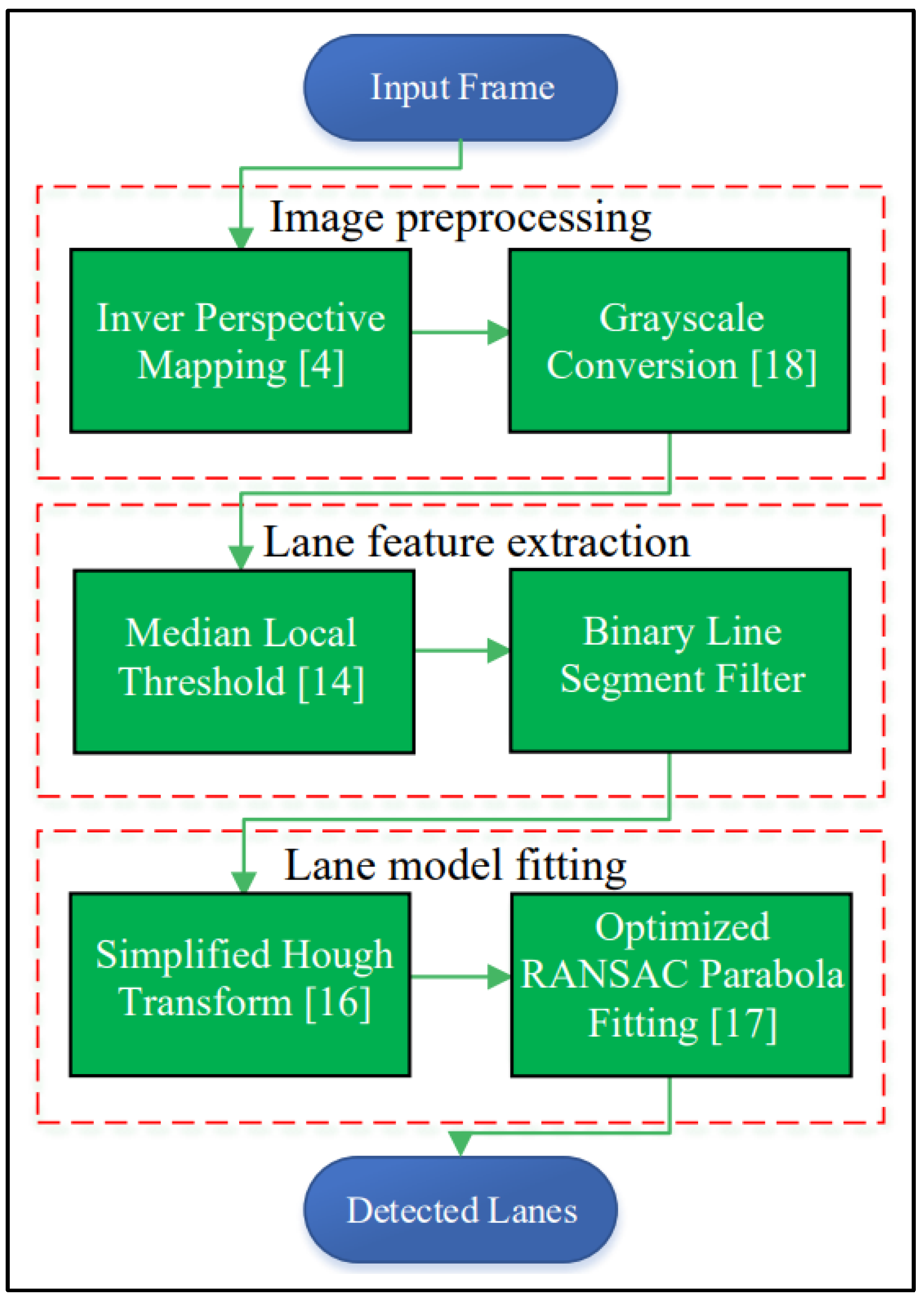
Figure 2.
An image sensor (dash-cam) with the camera coordinates mounted on a vehicle at height h above ground with pitch angle , yaw angle , and the offset from the vehicle center in the world coordinates
Figure 2.
An image sensor (dash-cam) with the camera coordinates mounted on a vehicle at height h above ground with pitch angle , yaw angle , and the offset from the vehicle center in the world coordinates
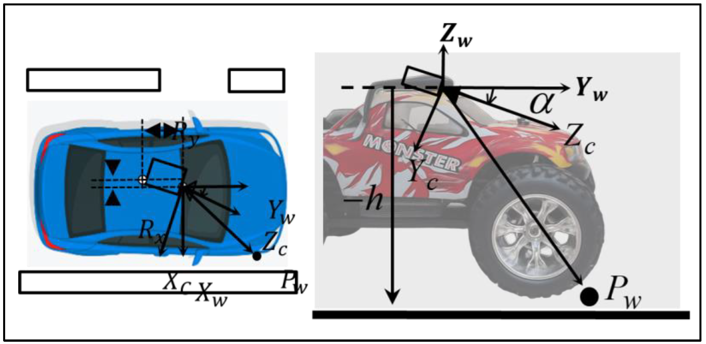
Figure 3.
Illustration of an input image by applying inverse perspective mapping to transform (a) a region of interest (in box) to (b) the bird’s eye view image so as to obtain parallel lane markings by (c) the projection of point to point on the ground.
Figure 3.
Illustration of an input image by applying inverse perspective mapping to transform (a) a region of interest (in box) to (b) the bird’s eye view image so as to obtain parallel lane markings by (c) the projection of point to point on the ground.
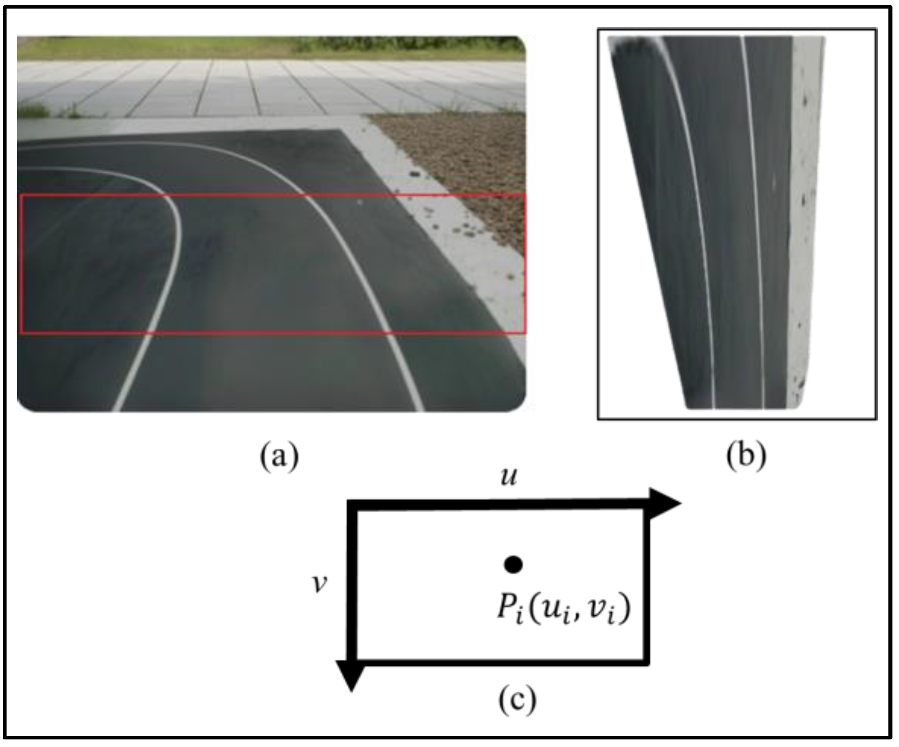
Figure 4.
Illustration of lane feature extraction by the median local threshold technique: (a) the grayscale image before the median local threshold processing; (b) the grayscale image after the median local threshold processing; and (c) the intensity distribution of a row in (a) before (solid line) and after (dashed line) applying the median local threshold.
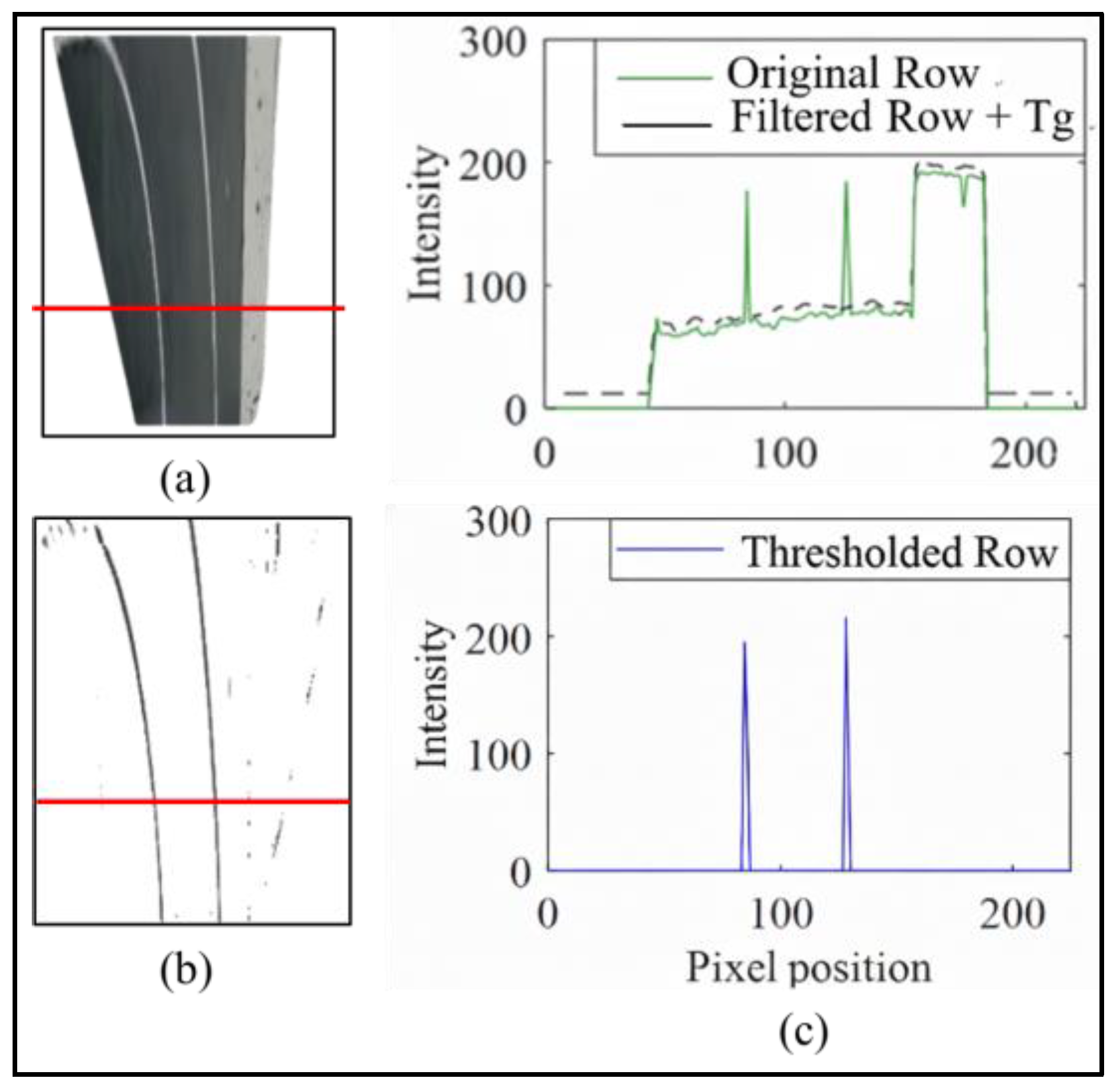
Figure 5.
Illustration of the binary line segment filter by calculating the level-line field, line support regions, and the length and angle of the line segment in the image from the median local threshold (b) to (c) and to filter the line segment of too short and of abnormal slope into (d).
Figure 5.
Illustration of the binary line segment filter by calculating the level-line field, line support regions, and the length and angle of the line segment in the image from the median local threshold (b) to (c) and to filter the line segment of too short and of abnormal slope into (d).
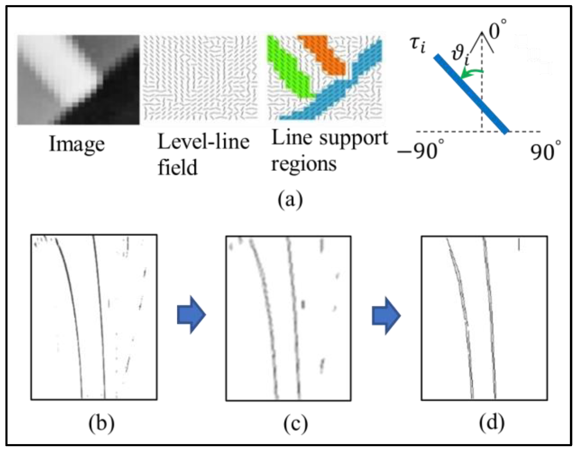
Figure 6.
Illustration of lane model fitting (a) by identifying lane width from the column intensity sum at the right/left lane markings and , (b) by locating the position of the sliding windows of the right/left lane markings with simplified Hough transform, and (c) by fitting the lane markings with the optimized RANSAC.
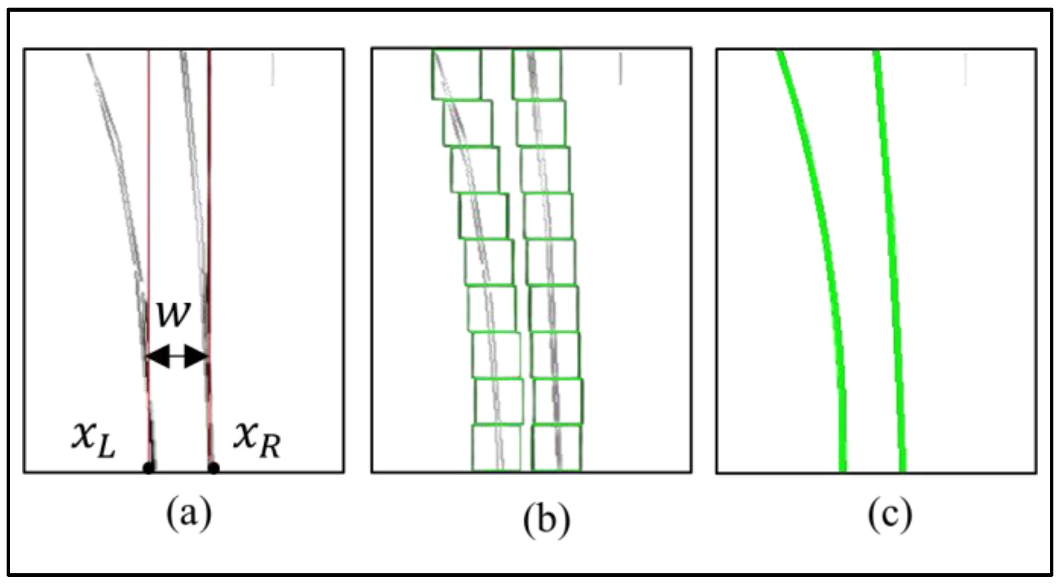
Figure 7.
The histogram analysis to determine the threshold in the binary line segment filter, (a) in left curved lane with angle distribution in and (b) in the straight lane with angle distribution in .
Figure 7.
The histogram analysis to determine the threshold in the binary line segment filter, (a) in left curved lane with angle distribution in and (b) in the straight lane with angle distribution in .
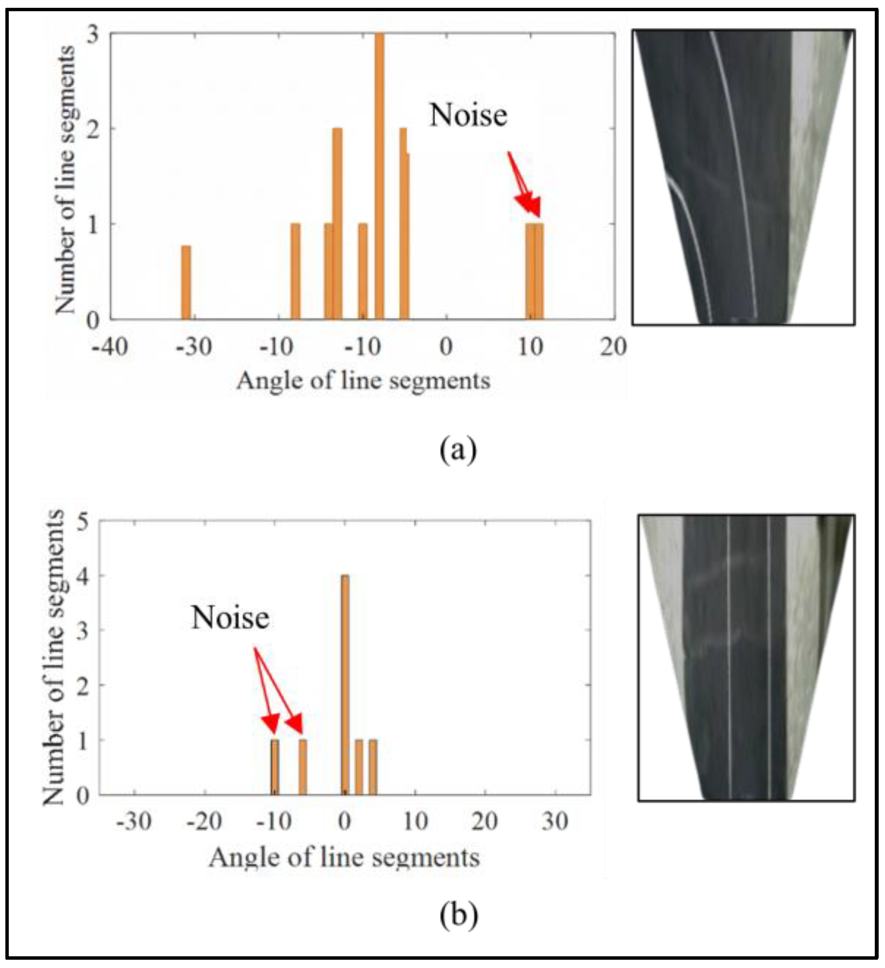
Figure 8.
Comparison of the lane feature extraction in (a) high curvature, (b) strong backlighting, (c) low contrast night, and (d) heavy rain by the algorithm of this work, [6,8,11].
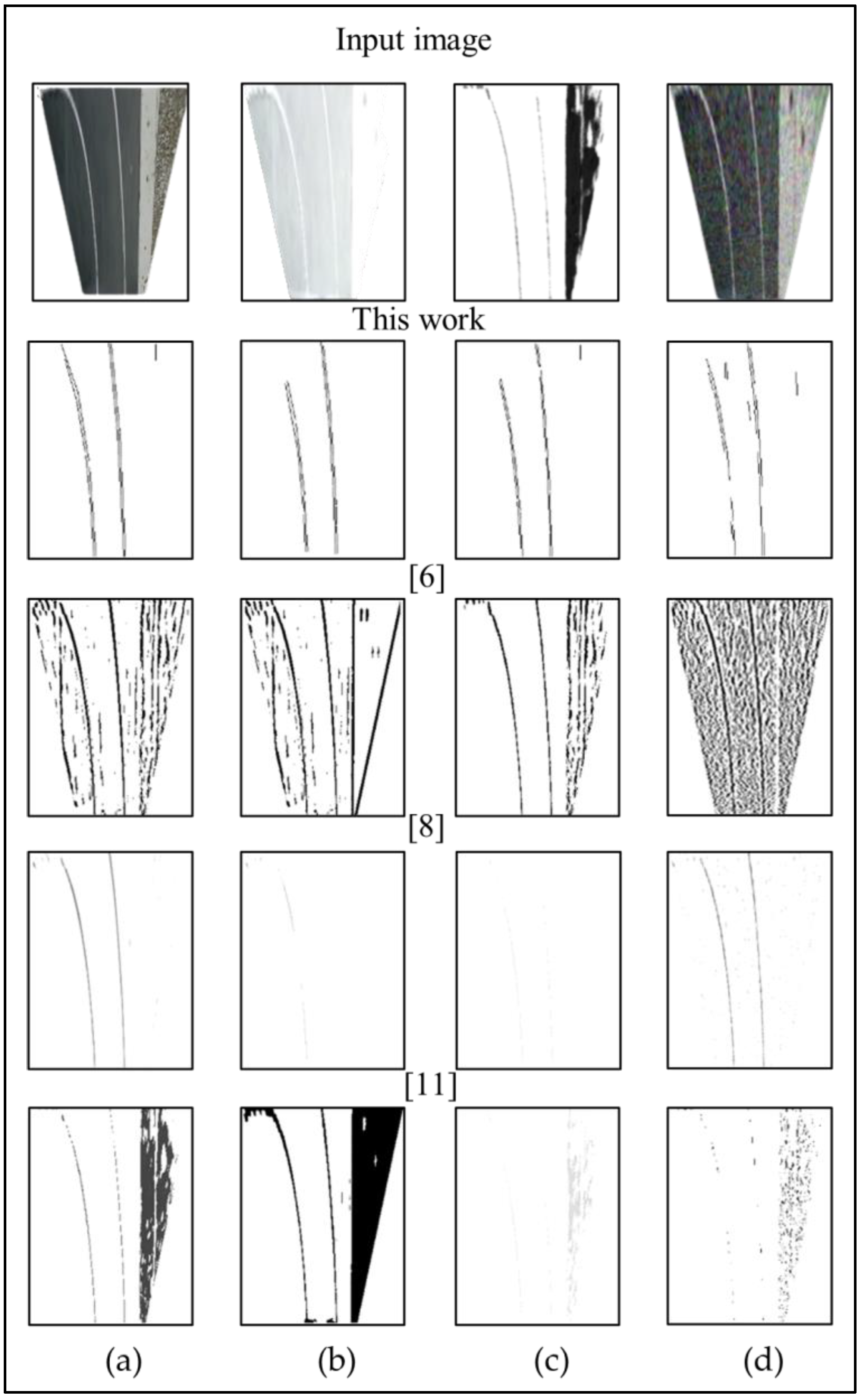

Table 1.
Comparison of the correct rate (%) of lane detection algorithm with and without the binary line segment filter (BLSF) by this work and by Kuo et al. [12].
Table 1.
Comparison of the correct rate (%) of lane detection algorithm with and without the binary line segment filter (BLSF) by this work and by Kuo et al. [12].
| Condition | With BLSF | Without BLSF | [12] |
|---|---|---|---|
| High curvature | 99% | 97% | 19% |
| Strong backlighting | 93% | 89% | 3% |
| Low contrast night | 92% | 92% | 36% |
| Heavy rain | 95% | 78% | 17% |
Table 2.
Quantitative comparison on the CULane and LLAMAS subsets. All methods are evaluated on the Dazzling Light and Night categories using the same BEV resolution and ROI. The proposed BLSF pipeline is compared against a geometric baseline [12], an ablation baseline (LSD w/o BLSF), and two lightweight deep learning models (UFLD [9], ENet-SAD [10] ). FPS is measured on the target 2 GHz ARM CPU platform without discrete GPU acceleration.
| Method | Backbone / Type | Dazzling Light (F1-score / IoU) | Night (F1-score / IoU) | FPS (CPU) | Power Efficiency |
|---|---|---|---|---|---|
| BLSF (Ours) | Geometric (LSD) | 0.861 / 0.792 | 0.847 / 0.774 | 30.6 | High |
| Baseline (No BLSF) | Geometric (LSD) | 0.801 / 0.776 | 0.776 / 0.731 | 29.2 | High |
| Kuo et al. [12] | Geometric (Grid) | 0.654 / 0.582 | 0.698 / 0.610 | 28.5 | High |
| UFLD [9] | DL (ResNet-18) | 0.872 / 0.805 | 0.855 / 0.781 | 8.4 | Low |
| ENet-SAD [10] | DL (ENet) | 0.841 / 0.763 | 0.832 / 0.755 | 14.1 | Medium |
Disclaimer/Publisher’s Note: The statements, opinions and data contained in all publications are solely those of the individual author(s) and contributor(s) and not of MDPI and/or the editor(s). MDPI and/or the editor(s) disclaim responsibility for any injury to people or property resulting from any ideas, methods, instructions or products referred to in the content. |
© 2025 by the authors. Licensee MDPI, Basel, Switzerland. This article is an open access article distributed under the terms and conditions of the Creative Commons Attribution (CC BY) license (http://creativecommons.org/licenses/by/4.0/).
Copyright: This open access article is published under a Creative Commons CC BY 4.0 license, which permit the free download, distribution, and reuse, provided that the author and preprint are cited in any reuse.


