
Submitted:
15 December 2025
Posted:
16 December 2025
You are already at the latest version
Abstract
This study investigates hydro-meteorological trends in five Alpine catchments within the Upper Po River basin, spanning Northwestern Italy and Southern Switzerland. We ana-lyzed climatic variables from 25 weather stations (1950–2022) alongside streamflow data from 14 river sections (1911–2022). Trends were assessed using the Mann-Kendall test to detect monotonic changes and the Theil-Sen estimator to quantify magnitude, ensuring robustness against outliers. Results reveal pronounced warming, particularly in spring maximum temperatures (+0.95 °C per decade). Conversely, average and minimum daily temperatures show lower rates (+0.50 and +0.39 °C per decade). Consequently, potential evapotranspiration increased significantly (+15.1 mm per decade), contributing to a marked decline in summer streamflow in 8 out of 14 sections. Correlation analysis con-firms that snow dynamics modulate the hydrological response: while precipitation drives discharge annually and in autumn, winter exhibits a weaker coupling, as winter precipi-tation is partially stored in the basin as snow, contributing to discharge during spring and summer. By focusing on this strategic region for European agriculture and industry, the study provides essential insights to support effective adaptation strategies.
Keywords:
climate change
; time series
; Alps
; streamflow
; trend
; correlation analysis
1. Introduction
Mountain areas are considered a hot spot for Climate Change [1]. Rising temperatures threaten diverse ecosystems, water supplies, and natural resources. Moreover, mountain areas host many glaciers that are retreating at global scale [2], serving as a visible proof of climate changes. Among all the mountain areas, the European Alps are one of the most studied. This is due to their proximity to a densely populated area, where technological development and scientific knowledge were relatively advanced during the last centuries. This enabled the reconstruction of climate series starting from the 18th century [3] These records revealed that during the 20th century, temperatures in the Alps increased at twice the global average (+2 °C vs +1 °C), with warming accelerating significantly since the 1980s. Consequently, this decade is widely considered a turning point for the Alps in terms of air temperature, sunshine duration, and snow cover [4,5,6], a shift largely attributed to water vapor-enhanced greenhouse warming [7].
In the European Alps, the compounding effects of climate change and dense urbanization are already causing significant economic and socio-environmental damage. Declining snow cover and the retreat of glaciers are negatively impacting winter tourism [8] while reducing summer river discharge. This poses a potential threat to key sectors such as agriculture [9] and hydropower [10]. Furthermore, extreme events, including storms, floods, droughts, and heat waves, are increasing in intensity and frequency [11,12], exposing goods, structures, and public services to damage.
These effects are also evident in the Italian sector. The Piedmont region’s environmental protection agency, ARPA Piemonte, highlighted a pronounced trend in regional maximum temperatures, which reached +0.58 °C per decade during 1981–2019 [13]. According to ARPA and ISPRA (the Italian Institute for Environmental Protection and Research), the years 2022-2024 were three of the four warmest years between 1958 and 2024. As in surrounding regions, average air temperatures show a significant warming trend [14], which also impacts groundwater temperature [15]. In contrast, high variability in total precipitation masks any clear long-term trend in annual average [16]. Nevertheless, extreme precipitation events are getting increasingly frequent. The winter of 2021-22 was the 3rd driest in the last 65 years, whereas October 2nd 2020 marked the wettest day in the last 60 years [17]. Similarly, the winter of 2022-23 was exceptionally dry, while 2024 ranked as the second wettest year in the historical records [18]. This variability has had profound implications for the river network. Notably, the severe snow drought of 2021–2022 resulted in the lowest terrestrial water storage on record during the summer of 2022 [19]. Molina et al. [20] suggested that the long-term deficit observed in the Po River between 2000 and 2022 might represent the most severe hydrological drought sequence in the last 500 years.
Given the intensification of extreme events, this study analyzes meteo-hydrological trends in the north-western Alps, specifically within a transboundary region spanning Northern Italy and Southern Switzerland. Unlike previous research in this area [14,15,16], which examined single variables in isolation, this study investigates the interplay temperature, precipitation and river discharge. While the link between precipitation and discharge could be considered intuitive, several factors, including the cryosphere cycle, the presence of reservoirs, crop demand, and changes in evapotranspiration, can weaken this link. To address this, we employed statistical correlation analysis to assess the response of flow discharge to climatic drivers within the studied catchment.
2. Materials and Methods
2.1. Study Area
The study area is located in the SW Alps, spanning northern Italy and southern Switzerland. It covers a total area of 12’665 km2 with complex orography [21]. Geographically, the region encompasses a large portion of Piedmont, western Lombardy, and the Swiss cantons of Valais and Ticino (Figure 1). It comprises five major sub-basins (Ticino, Sesia, Toce, Agogna, and Terdoppio Novarese), all tributaries of the Po River. The mean elevation of these basins ranges from 137 m a.s.l. (Terdoppio) to 1548 m a.s.l. (Toce), with an average elevation of 870 m a.s.l. across the entire study area (Table 1). Catchment sizes vary significantly, ranging from 515 km2 (Terdoppio) to 6,301 km2 (Ticino).
2.2. Data
Daily data for rainfall, temperature, estimated evapotranspiration, and river discharge were aggregated into annual and seasonal time series. The seasonal periods were defined as: Winter (JFM), Spring (AMJ), Summer (JAS), and Autumn (OND). All datasets underwent quality control to filter incomplete years and remove outliers (i.e., physically implausible values). Following established protocols [22], we required a minimum monthly data availability of ≥ 80% for precipitation and ≥ 50% for temperature and discharge. Consequently, any annual or seasonal record containing one or more missing or incomplete months was excluded from the analysis.
2.2.1. Climate Data
Precipitation and air temperature data were sourced from two distinct datasets. For the trend analysis (Section 3.2), we utilized 25 daily time series of precipitation and temperature (minimum, average, maximum) from stations in Switzerland and Italy (Piedmont and Lombardy) (Figure 1, Table SM1). These data, aggregated to a monthly resolution, cover the period 1979–2022. Swiss data were provided by MeteoSwiss, while Italian data were retrieved from automatic stations managed by ARPA Lombardia and ARPA Piemonte. Most series span at least 30 years, with minor exceptions in data-scarce areas. Station elevations range from 155 m a.s.l. to 2,820 m a.s.l.
For the correlation analysis (Section 4.6), we employed a monthly gridded dataset covering the period 1900–2021, based on an enhanced version of the dataset presented in [23]. This dataset features a spatial resolution of 30 arc-seconds and was reconstructed using the anomaly method. This involved superimposing relative anomaly series onto a high-resolution 1961–1990 climatology. The anomaly series were derived by interpolating a high-density dataset of quality-controlled precipitation records, which integrates data from historical mechanical stations, owned by the Italian Hydrological Service, and modern automatic stations, managed by regional authorities.
2.2.2. Hydrometric Data
To assess trends and correlations with climate variables, we selected 14 hydrometric stations (Figure 2, Table SM2) distributed across five main catchments: Agogna, Sesia, Terdoppio Novarese, Toce, and Ticino. These stations provide daily discharge records. Due to the steep topography of the Alpine terrain, the hydrological response is fast, with times of concentration generally shorter than 24 hours [24].
Complementing the river discharge data, we analyzed water level records from Lake Maggiore, measured at Sesto Calende near the lake’s outlet. This dataset was examined to identify potential trends driven by climatic shifts or changes in the regulation of the Miorina dam.
2.3. Methods
2.3.1. Evapotranspiration Assessment
Based on the temperature datasets described in Section 3.1, we calculated monthly series of Potential Evapotranspiration (PET) for all weather stations and grid points. These estimates were derived using the Thornthwaite equation [25,26]:
[1]
where PET is the potential evapotranspiration [mm/month] for a specific month i, and Tmean denotes the average monthly temperature [°C] (adjusted to 0 °C if negative). Finally, I is the annual heat index, calculated according to the following equation:
[2]
The exponent a is an empirical coefficient dependent on the annual heat index I, calculated as follows:
[3]
2.3.2. Water Storage of Lake Maggiore
We could exploit the available data of inflow, QIN (given by the sum of discharge of main tributaries: CN, LS, LA, BE, PT), outflow, and QOUT (assessed at DM), to calculate water storage for Lake Maggiore:
[4]
where ∆V is the lake volume variation as due to the balance of inflow and outflow within the time window ∆t considered, i.e., 1 day. To calculate the daily regulation volume, we defined a reference volume of 0 Mm3 corresponding to a water level of -0.50 m. This level represents the minimum value observed in the historical record relative to the hydrometric zero (193.01 m a.s.l.).
2.3.3. Effects of Flow Regulation
In the Alpine region, hydropower infrastructure is widespread [27]. These structures can significantly alter hydrological regimes by modifying downstream flow. Four of the selected gauging stations are situated downstream of major dams (Figure 1, Table 2), potentially subjecting their discharge records to anthropogenic alteration. However, the catchments upstream of the Sosto, Isola, and Sambuco dams account for less than 20% of the total contributing area at the corresponding gauging stations [28]. Consequently, their regulatory impact can be neglected as a first approximation. In contrast, the Miorina dam regulates a much larger drainage area; therefore, its influence on discharge dynamics requires specific investigation.
2.3.4. Detection of Significant Trends
To identify significant trends in seasonal precipitation, temperature, and evapotranspiration, we applied the non-parametric Mann-Kendall (M-K) test with a significance level of . This test is widely employed in climatological and hydrological studies [29,31]to detect monotonic trends within time series. Methodologically, the test involves comparing the rank of each data point with all subsequent values, utilizing the sign function to determine the direction of the change.
[5]
Under the null hypothesis of no monotonic trend, the test statistic follows a standard normal distribution. However, while the M-K test identifies the significance of a trend, it does not quantify its magnitude. To address this, we coupled the M-K test (significance level ) with the Theil-Sen estimator [32,33]. This method calculates the magnitude of the trend as the median slope of all possible pairs of data points. Unlike simple linear regression, the Theil-Sen estimator is highly robust against outliers [34], making it particularly suitable for hydro-meteorological time series.
2.3.5. Correlation Analysis Between Surface Runoff and Climatic Variables
Finally, we investigated the correlation between mean seasonal river discharge and climatic drivers (precipitation, temperature, and evapotranspiration). As noted, this analysis utilized the gridded dataset rather than point-station data. For each catchment, we calculated spatially averaged values of temperature, precipitation, and evapotranspiration by aggregating grid cells within the respective watershed boundaries. To ensure robustness, we employed three distinct statistical metrics: Pearson’s correlation coefficient [35], Spearman’s rank correlation coefficient [36], and Kendall’s rank correlation coefficient [37]. The analysis focused exclusively on concurrent (zero-lag) correlations between seasonal hydro-climatic variables. Specifically, discharge records from the selected stations were correlated with the area-averaged climatic data for the catchments depicted in Figure 1.
3. Results
3.1. Mean Hydro-Climatic Conditions
As a preliminary step to the trend and correlation analysis, we present the long-term climatological baseline of the study area. Figure 3 illustrates the minimum, mean, and maximum daily temperatures, which exhibit a strong dependence on station elevation. Complementing this, Figure 4 depicts the average values for Potential Evapotranspiration (PET), total precipitation, and river discharge.
3.2. Trend Analysis
The results of the trend analysis and their statistical significance are summarized in Figure 5 and Figure 6, and listed in detail in Tables SM3-9. Precipitation, characterized by high natural variability, generally lacks significant long-term trends (Table SM3, Figure 6). However, a localized negative trend in summer (JAS) precipitation was observed in 5 out of 25 stations. In contrast, temperature (Tables SM4-6, Figure 5) and PET (Table SM7, Figure 6) exhibit clear positive trends. The most pronounced warming occurs in spring, particularly for maximum daily temperature (+0.95 °C per decade). Conversely, winter (JFM) temperature trends are smaller in magnitude and less statistically significant. River discharge (Figure 6, Table SM8) shows significant negative trends in 10 out of 15 stations, primarily in summer (JAS), a pattern likely driven by increasing PET. Weak positive trends were observed in winter (JFM), possibly due to a shift from snowfall to rain. regarding Lake Maggiore, the analysis of water levels and volumes revealed no significant trends (Table SM9). The absence of trends in the lake parameters implies that reservoir regulation does not significantly alter downstream flow dynamics at the seasonal scale. Notably, while significant trends exist in the discharge downstream of the Miorina dam, the lake’s storage volume remains stable. This strongly suggests that the observed downstream trends are not artifacts of management policies, but are driven by upstream climatic conditions
3.3. Correlation Analysis
The calculated correlation coefficients (Pearson, Spearman, and Kendall) were in close agreement, yielding very similar values in this study. Given the expected linear dependence between the analyzed variables and Pearson’s wider adoption in this field [28], only the results of the Pearson’s correlation coefficient (r) are reported (Table 3 and Table 4). Flow discharge was correlated against the spatially averaged climate data (Section 3.3) for the 14 catchments (Figure 1).
Pearson’s r generally exhibits high coefficients, confirming a strong linear relationship between discharge and climatic variables. Correlation values against precipitation are high across all seasons, especially at yearly scale, with peaks reaching . Maximum temperatures reveal primarily negative correlations, indicating that as maximum temperature rises, river discharge tends to decrease. Likewise, minimum temperature shows generally negative correlation in spring (AMJ) and summer (JAS) but positive correlation in autumn (OND) and winter (JFM).
4. Discussion
4.1. Climate Trends in Alpine Area
As highlighted in the introduction, the European Alps are experiencing warming rates twice the global average [3], with summer trends generally exceeding those in winter (Tables SM4-6). In terms of winter dynamics, our results are consistent with observations from the Swiss and French Alps [38,40], which identify stronger warming at lower elevations. Indeed, we found consistent winter warming trends exclusively at stations located below 600 m a.s.l.. Regarding summer trends, the cited studies [38,40] report stronger warming above 2000 m a.s.l.. However, in our study area, we did not detect such Elevation-Dependent Warming (EDW); instead, summer temperature increases appear variable across all stations regardless of altitude
Our dataset is characterized by wide variability in the start year of measurements, while the end year for almost all stations is 2022. Due to this temporal heterogeneity, the calculated average trend (+0.50 °C per decade), while substantial in magnitude, has limited statistical representativeness as it aggregates different timeframes. However, a clear pattern emerges when grouping by observation period: stations with records starting in the 1950s (MC, LU, LM) show moderate trends (+0.20 to +0.39 °C per decade), whereas for stations beginning after the 1980s, the trend is substantially steeper. This confirms that climate change has intensified during the last few decades [4,5,41].
Regarding daily maximum and minimum temperatures, we observed a stronger warming trend for the maximums compared to the minimums. This contrasts with Acquaotta et al. [14], who reported larger trends for minimum temperatures in the North-Western Alps. However, Stucchi et al. [5]—analyzing a subset of the same data—excluded maximum temperatures, citing potential biases from older equipment and direct solar radiation [42]. Our findings align more closely with Nigrelli and Chiarle [43], who analyzed 23 Alpine stations and reported decadal increases of 0.5 °C for maximum and 0.4 °C for minimum temperatures. Notably, they also found no significant correlation between elevation and warming rates, consistent with the absence of EDW in our results.
Precipitation exhibits the highest variability in the dataset, showing no significant trend on an annual scale. However, a significant negative trend in summer was detected in 5 out of 25 stations. Similar negative summer trends have been reported in the SE and Southern Alps [44,45], although those regions also show positive winter trends that are absent in our study area. Consistent with the precipitation signal, river discharge shows no generalized annual trend but a significant decline in summer (Table 10). Unlike other Alpine regions, our study area is characterized by limited glacial coverage. Consequently, the earlier onset of snowmelt [46,48] combined with increasing potential evapotranspiration (Table SM7) drives the reduction in summer discharge [49]. This interpretation is further supported by the high correlation coefficients observed between summer temperature and flow, which reinforce the causal link between these variables.
The correlation analysis confirmed the relationship between discharge and precipitation, which is strongest at the annual scale. At the seasonal scale, snow dynamics (accumulation and melt) significantly modulate the hydrological response. Notably, the coupling between precipitation and discharge is weakest in winter. Indeed, the observed positive correlation between minimum temperature and winter discharge confirms that colder temperatures favor snow accumulation, effectively storing water and reducing immediate runoff. On the other hand, we observe for 14 out of 15 river sections a negative correlation in summer between discharge and temperature, due to enhanced evapotranspiration losses. Notably, this negative correlation is more pronounced for maximum temperature and displays significant spatial heterogeneity across catchments (e.g., for Ticino at BO vs. for Maggia at LS). This variability highlights the need for site-specific analyses to elucidate the complex interplay between temperature and discharge. For instance, in high-altitude catchments, the persistence of snow cover may attenuate the negative correlation driven by evapotranspiration, as higher temperatures also induce meltwater release. Furthermore, hydropower reservoir operations, which release water based on energy demand, can decouple the natural relationship between climatic drivers and river discharge.
Conclusions
This study advances the understanding of hydro-climatic trends and their impact on Alpine river discharge. Our analysis confirms that the Alpine region is warming at a rate double the global average. This warming is characterized by a distinct asymmetry, with maximum temperatures rising faster than minimums, leading to an increased diurnal temperature range in 19 out of 25 stations. These climatic shifts have profound hydrological implications. The accelerated warming, particularly in spring and summer, drives a significant increase in potential evapotranspiration, which correlates with the observed decline in summer streamflow. Simultaneously, the positive correlation between winter temperature and discharge signals a structural shift in the hydrological regime: Alpine catchments are transitioning from nival (snow-dominated) to pluvial (rain-dominated) behaviors. This transition reduces natural water storage in the form of snowpack, altering the timing of water availability for the downstream European plains. By focusing on the Upper Po River basin—a strategic resource for Northern Italian agriculture and industry—this work provides the quantitative basis needed to define effective adaptation strategies to cope with increasingly scarce summer resources.
Supplementary Materials
The following supporting information can be downloaded at the website of this paper posted on Preprints.org.
Author Contributions
Conceptualization, D.J., L.S. and D.B.; methodology, V.M., M.M.; formal analysis, D.J., L.S.; writing—original draft preparation, D.J., L.S.; writing—review and editing, L.S., D.B., V.M., M.M. . All authors have read and agreed to the published version of the manuscript.” Please turn to the CRediT taxonomy for the term explanation. Authorship must be limited to those who have contributed substantially to the work reported.
Funding
This research received no external funding.
Data Availability Statement
All data are available on reasonable request and can be downloaded from ARPA Piemonte and MeteoSwiss.
Acknowledgments
To recognize the invaluable time, effort, and attention to detail that each review contained, the authors express their sincere gratitude to the reviewers.
Conflicts of Interest
The authors declare no conflicts of interest.
References
- Mountains. Climate Change 2022 – Impacts, Adaptation and Vulnerability; Cambridge University Press, 2023; pp. 2273–2318. [Google Scholar]
- Zemp, M.; Huss, M.; Thibert, E.; Eckert, N.; McNabb, R.; Huber, J.; Barandun, M.; Machguth, H.; Nussbaumer, S.U.; Gärtner-Roer, I.; et al. Global Glacier Mass Changes and Their Contributions to Sea-Level Rise from 1961 to 2016. Nature 2019, 568, 382–386. [Google Scholar] [CrossRef] [PubMed]
- Auer, I.; Böhm, R.; Jurkovic, A.; Lipa, W.; Orlik, A.; Potzmann, R.; Schöner, W.; Ungersböck, M.; Matulla, C.; Briffa, K.; et al. HISTALP—Historical Instrumental Climatological Surface Time Series of the Greater Alpine Region. International Journal of Climatology 2007, 27, 17–46. [Google Scholar] [CrossRef]
- Steiger, R.; Knowles, N.; Pöll, K.; Rutty, M. Impacts of Climate Change on Mountain Tourism: A Review. Journal of Sustainable Tourism 2024, 32, 1984–2017. [Google Scholar] [CrossRef]
- Bocchiola, D. Impact of Potential Climate Change on Crop Yield and Water Footprint of Rice in the Po Valley of Italy. Agric Syst 2015, 139, 223–237. [Google Scholar] [CrossRef]
- Gaudard, L.; Romerio, F.; Dalla Valle, F.; Gorret, R.; Maran, S.; Ravazzani, G.; Stoffel, M.; Volonterio, M. Climate Change Impacts on Hydropower in the Swiss and Italian Alps. Science of The Total Environment 2014, 493, 1211–1221. [Google Scholar] [CrossRef] [PubMed]
- Wilhelm, B.; Rapuc, W.; Amann, B.; Anselmetti, F.S.; Arnaud, F.; Blanchet, J.; Brauer, A.; Czymzik, M.; Giguet-Covex, C.; Gilli, A.; et al. Impact of Warmer Climate Periods on Flood Hazard in the European Alps. Nat Geosci 2022, 15, 118–123. [Google Scholar] [CrossRef]
- Le Roux, E.; Evin, G.; Eckert, N.; Blanchet, J.; Morin, S. Elevation-Dependent Trends in Extreme Snowfall in the French Alps from 1959 to 2019. Cryosphere 2021, 15, 4335–4356. [Google Scholar] [CrossRef]
- Avato, M.T. RELAZIONE ANNUALE 2020 VERSO UN PRESENTE SOSTENIBILE II 2020.
- Acquaotta, F.; Fratianni, S.; Garzena, D. Temperature Changes in the North-Western Italian Alps from 1961 to 2010. Theor Appl Climatol 2015, 122, 619–634. [Google Scholar] [CrossRef]
- Egidio, E.; Mancini, S.; De Luca, D.A.; Lasagna, M. The Impact of Climate Change on Groundwater Temperature of the Piedmont Po Plain (NW Italy). Water (Basel) 2022, 14, 2797. [Google Scholar] [CrossRef]
- Acquaotta, F.; Fratianni, S. Analysis on Long Precipitation Series in Piedmont (North-West Italy). Am J Clim Change 2013, 02, 14–24. [Google Scholar] [CrossRef]
- ARPA Evento Del 2-3 Ottobre 2020. 2020.
- Arpa Piemonte. Il Clima in Piemonte 2024.; 2025.
- Fugazza, D.; Manara, V.; Senese, A.; Diolaiuti, G.; Maugeri, M. Snow Cover Variability in the Greater Alpine Region in the MODIS Era (2000–2019). Remote Sens (Basel) 2021, 13, 2945. [Google Scholar] [CrossRef]
Figure 1.
Map of the study area and Digital Terrain Model (DTM). The monitoring network includes dams (purple triangles), hydrometric stations (blue dots), and weather stations (red dots). Major watersheds (hatched areas), the river network, and lakes are also depicted.
Figure 1.
Map of the study area and Digital Terrain Model (DTM). The monitoring network includes dams (purple triangles), hydrometric stations (blue dots), and weather stations (red dots). Major watersheds (hatched areas), the river network, and lakes are also depicted.
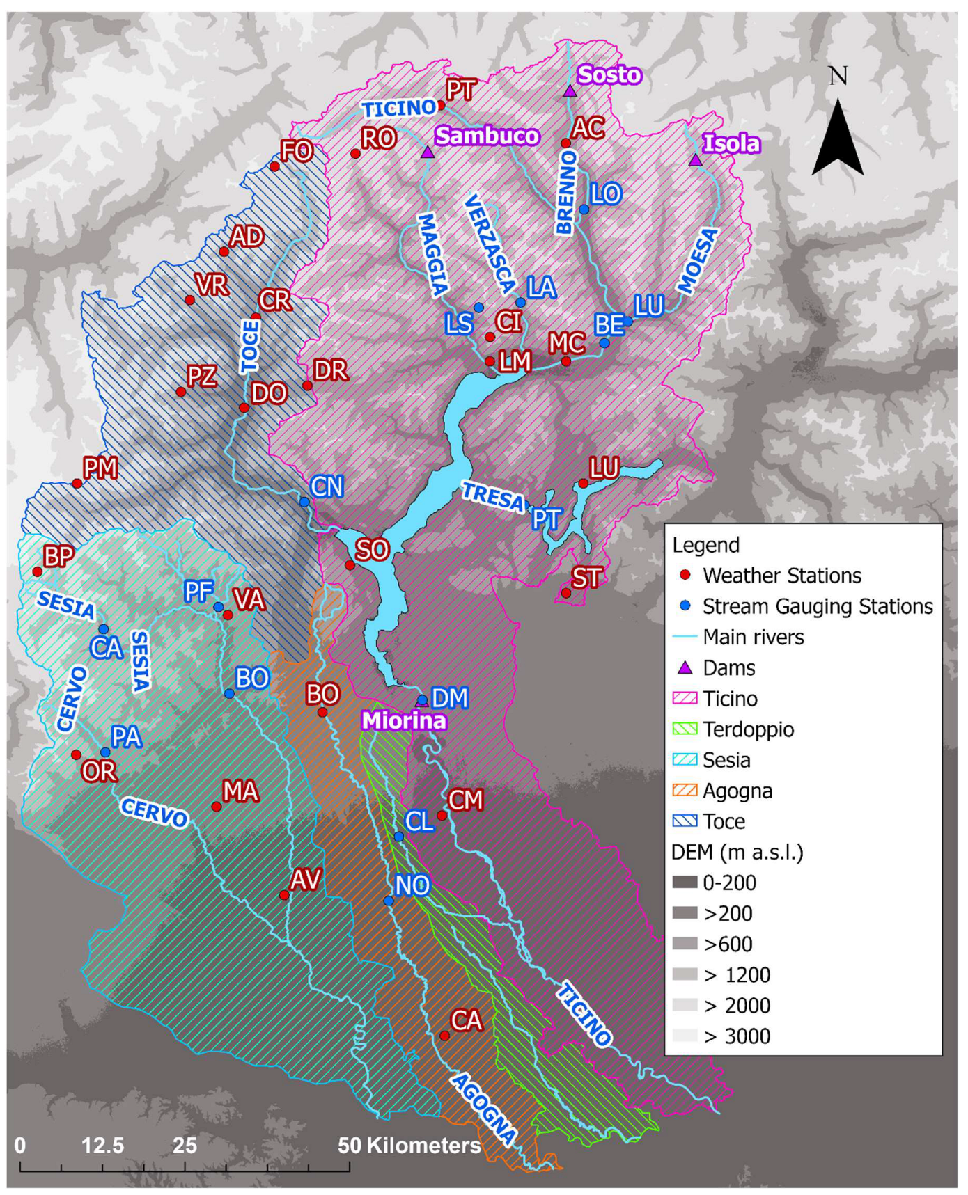
Figure 2.
Map of the stream gauging station catchments. Thick outlines delimit the five main basins. Downstream sub-basins (PB, NO, BO, MD) are distinguished by solid colors, whereas upstream sub-basins are highlighted with hatched patterns.
Figure 2.
Map of the stream gauging station catchments. Thick outlines delimit the five main basins. Downstream sub-basins (PB, NO, BO, MD) are distinguished by solid colors, whereas upstream sub-basins are highlighted with hatched patterns.
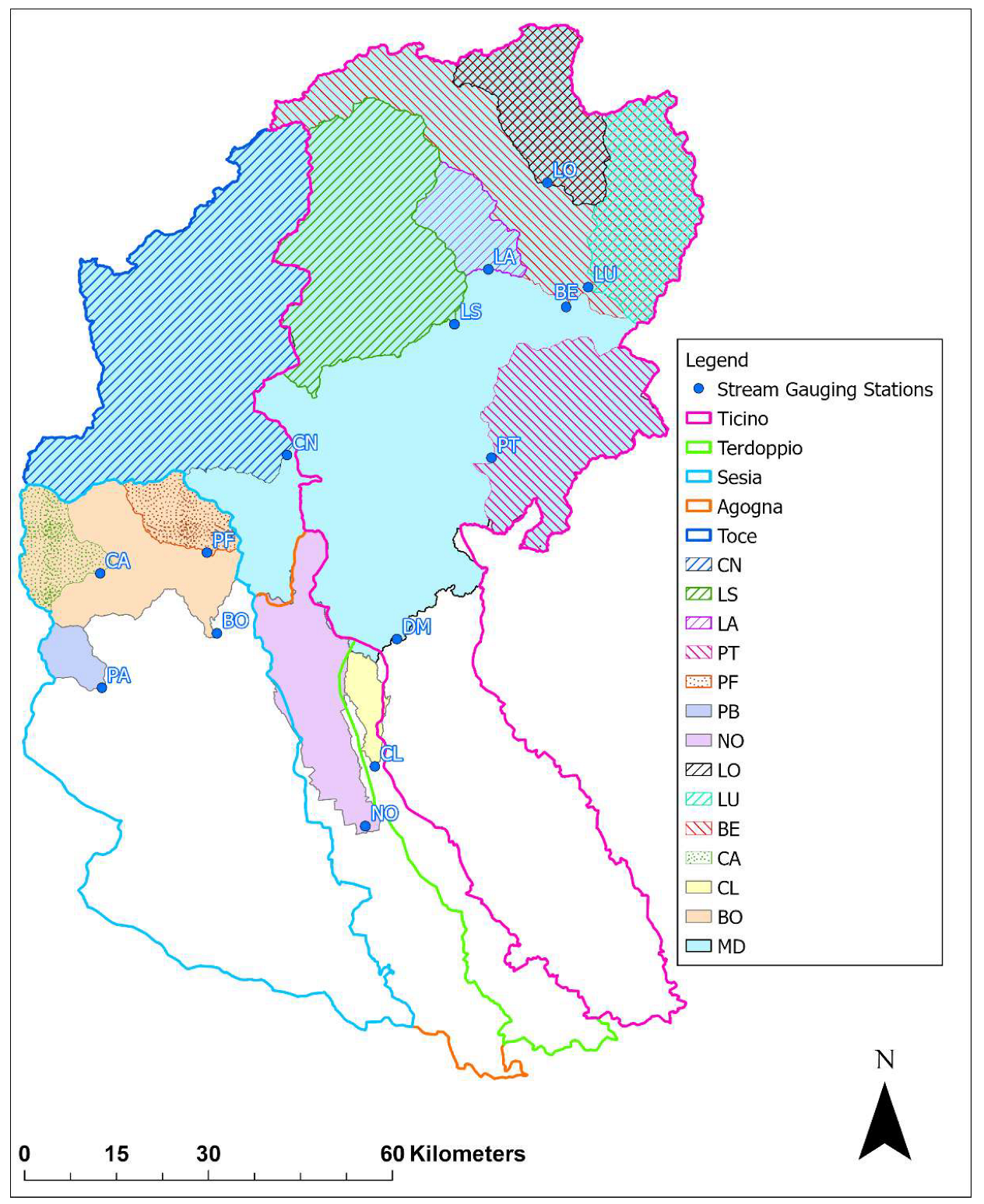
Figure 3.
Long-term daily temperature statistics. The chart displays the average minimum (green), mean (orange), and maximum (red) temperatures.
Figure 3.
Long-term daily temperature statistics. The chart displays the average minimum (green), mean (orange), and maximum (red) temperatures.
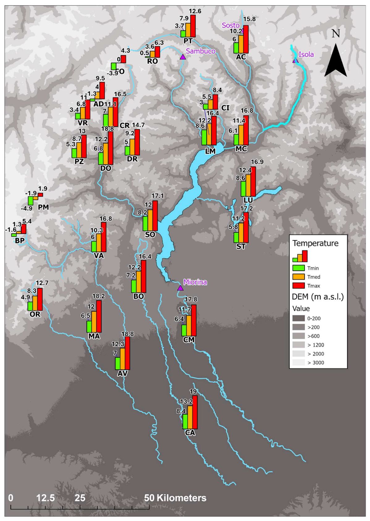
Figure 4.
Long-term mean annual hydro-climatic variables: Potential Evapotranspiration (PET, Thornthwaite method), total precipitation, and river discharge.
Figure 4.
Long-term mean annual hydro-climatic variables: Potential Evapotranspiration (PET, Thornthwaite method), total precipitation, and river discharge.
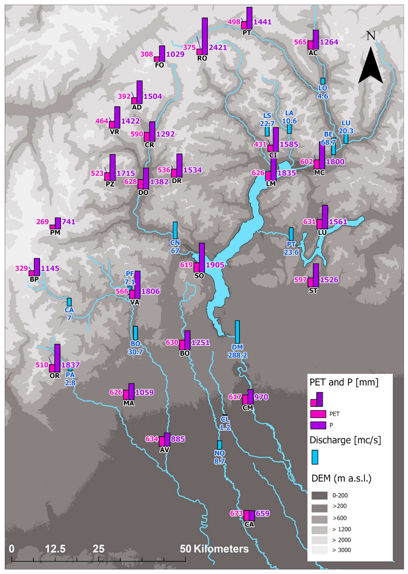
Figure 5.
Trends in annual minimum, mean, and maximum temperatures. Trend magnitudes are expressed in °C/decade. Numerical labels are displayed only for statistically significant results (p < 0.05).
Figure 5.
Trends in annual minimum, mean, and maximum temperatures. Trend magnitudes are expressed in °C/decade. Numerical labels are displayed only for statistically significant results (p < 0.05).
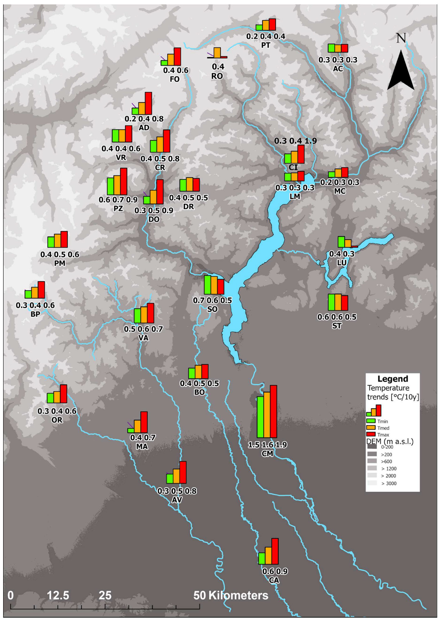
Figure 6.
Trends in annual precipitation, Potential Evapotranspiration (PET), and river discharge. Bars represent the trend magnitude. Statistically non-significant trends (p > 0.05) are distinguished by a hatched pattern.
Figure 6.
Trends in annual precipitation, Potential Evapotranspiration (PET), and river discharge. Bars represent the trend magnitude. Statistically non-significant trends (p > 0.05) are distinguished by a hatched pattern.
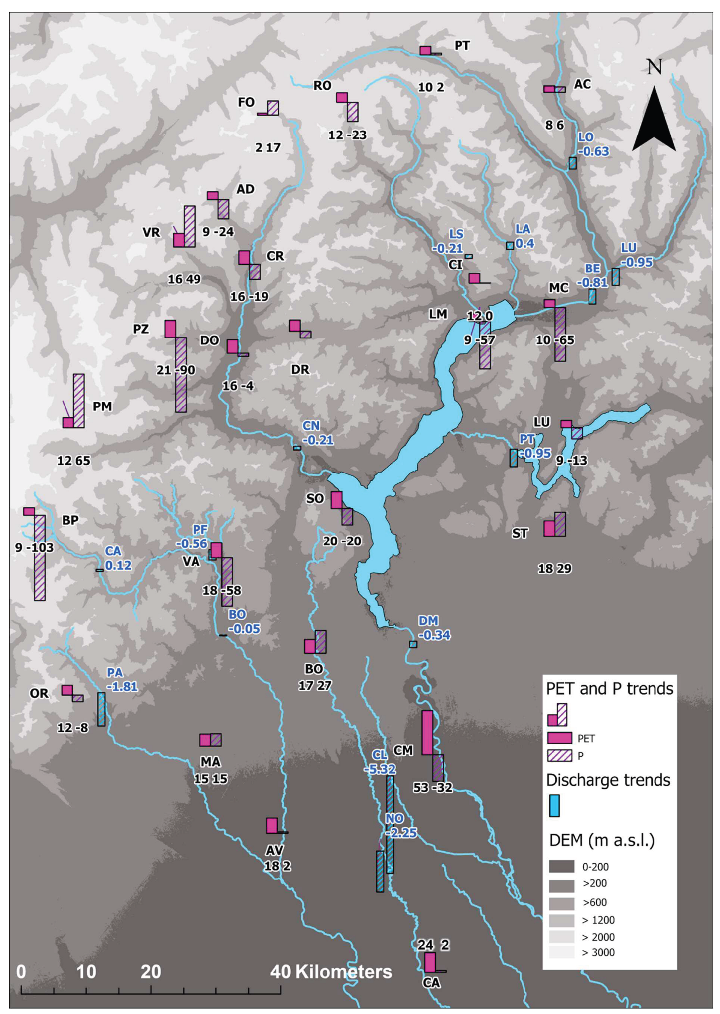

Table 1.
Main features of the chosen catchments (basins).
| # | Basin | Area [Km2] |
Mean Altitude [m a.s.l.] |
Max Altitude [m a.s.l.] |
Min Altitude [m a.s.l.] |
| 1 | Ticino | 6301 | 951 | 3401 | 53 |
| 2 | Toce | 1778 | 1548 | 4591 | 194 |
| 3 | Sesia | 3075 | 644 | 4542 | 92 |
| 4 | Agogna | 996 | 205 | 1175 | 64 |
| 5 | Terdoppio Novarese | 515 | 137 | 382 | 58 |
| Tot: | 12665 | 870 | 4591 | 53 |
Table 2.
Main features of the dams and the related hydrometric stations.
| # | Dam | Long. [m] | Lat. [m] |
A0 [m a.s.l.] |
Dam Catchment Area [Km2] | River | Stream Gauging Station | Reservoir Volume [Mm3] |
| 1 | Isola Dam | 9.1909 | 46.4475 | 1584 | 42 | Moesa | Lumino | 6.5 |
| 2 | Sosto Dam | 8.9414 | 46.5403 | 1023 | 80 | Brenno | Loderio | 0.02 |
| 3 | Miorina Dam | 8.6533 | 45.7061 | 194 | 6599 | Ticino | Miorina | 420 |
| 4 | Sambuco Dam | 8.6597 | 46.4561 | 1376 | 34 | Maggia | Locarno-Solduno | 64 |
Table 3.
Pearson correlation coefficients (r) between discharge and climatic variables (precipitation and PET). Cells are color-coded based on the correlation sign: green indicates positive correlation, while red indicates negative correlation. Note: “Lake Maggiore Input” denotes the aggregated inflow from the Ticino, Toce, Tresa, Maggia, and Verzasca rivers.
| Pearson Correlation Coefficient | |||||||||||
| River | ID | Rainfall | PET | ||||||||
| JFM | AMJ | JAS | OND | Yr | JFM | AMJ | JAS | OND | Yr | ||
| Agogna | NO | 0.40 | 0.62 | 0.71 | 0.82 | 0.83 | 0.25 | -0.15 | -0.31 | 0.08 | -0.21 |
| Cervo | CL | 0.84 | 0.84 | 0.68 | 0.93 | 0.90 | 0.05 | -0.16 | -0.28 | -0.02 | -0.12 |
| Mastallone | DM | 0.83 | 0.73 | 0.51 | 0.87 | 0.88 | 0.13 | -0.19 | -0.54 | 0.19 | -0.01 |
| Sesia | CN | 0.40 | 0.67 | 0.48 | 0.81 | 0.73 | 0.02 | 0.00 | -0.08 | 0.01 | -0.16 |
| Sesia | LS | 0.54 | 0.70 | 0.65 | 0.86 | 0.81 | -0.01 | -0.29 | -0.16 | -0.07 | -0.24 |
| Terdoppio | BE | 0.76 | 0.68 | 0.80 | 0.87 | 0.93 | 0.03 | -0.22 | -0.22 | 0.00 | -0.18 |
| Brenno | LU | 0.77 | 0.65 | 0.87 | 0.90 | 0.90 | 0.34 | -0.20 | -0.27 | -0.01 | -0.09 |
| Maggia | PT | 0.53 | 0.73 | 0.72 | 0.74 | 0.77 | 0.29 | -0.47 | 0.02 | -0.09 | -0.17 |
| Moesa | LO | 0.64 | 0.67 | 0.82 | 0.87 | 0.85 | 0.28 | -0.32 | -0.21 | -0.11 | -0.14 |
| Ticino | BO | 0.64 | 0.76 | 0.69 | 0.86 | 0.90 | 0.11 | -0.28 | -0.42 | 0.06 | -0.22 |
| Ticino | PF | 0.82 | 0.90 | 0.85 | 0.88 | 0.90 | 0.08 | -0.49 | -0.67 | 0.43 | -0.26 |
| Tresa | LA | 0.79 | 0.73 | 0.82 | 0.86 | 0.80 | -0.28 | -0.23 | -0.43 | 0.06 | -0.30 |
| Verzasca | PA | 0.83 | 0.72 | 0.84 | 0.85 | 0.90 | -0.04 | -0.36 | -0.64 | 0.17 | -0.29 |
| Toce | CA | 0.82 | 0.83 | 0.74 | 0.90 | 0.95 | 0.14 | -0.44 | -0.60 | 0.10 | -0.28 |
Table 4.
Pearson correlation coefficients (r) between discharge and temperature metrics (average, minimum, and maximum). Cells are color-coded based on the correlation sign: green indicates positive correlation, while red indicates negative correlation. Note: “Lake Maggiore Input” denotes the aggregated inflow from the Ticino, Toce, Tresa, Maggia, and Verzasca rivers.
| Pearson Correlation Coefficient | ||||||||||||||||
| River | ID | T MAX | T AVE | T MIN | ||||||||||||
| JFM | AMJ | JAS | OND | Yr | JFM | AMJ | JAS | OND | Yr | JFM | AMJ | JAS | OND | Y | ||
| Agogna | NO | 0.26 | -0.28 | -0.48 | -0.06 | -0.31 | 0.37 | -0.24 | -0.48 | 0.08 | -0.25 | 0.49 | -0.19 | -0.45 | 0.22 | -0.17 |
| Terdoppio | CL | -0.05 | -0.25 | -0.35 | -0.17 | -0.22 | 0.06 | -0.22 | -0.28 | 0.07 | -0.10 | 0.19 | -0.16 | -0.17 | 0.31 | 0.07 |
| Ticino | DM | 0.08 | -0.38 | -0.54 | -0.18 | -0.33 | 0.23 | -0.31 | -0.51 | 0.02 | -0.23 | 0.38 | -0.20 | -0.45 | 0.20 | -0.11 |
| Toce | CN | -0.04 | -0.54 | -0.65 | -0.19 | -0.39 | 0.14 | -0.48 | -0.60 | 0.04 | -0.30 | 0.35 | -0.33 | -0.51 | 0.25 | -0.17 |
| Maggia | LS | -0.02 | -0.50 | -0.21 | -0.21 | -0.28 | 0.04 | -0.49 | -0.19 | -0.08 | -0.23 | 0.14 | -0.38 | -0.15 | 0.07 | -0.16 |
| Ticino | BE | -0.10 | -0.56 | -0.68 | -0.01 | -0.33 | 0.09 | -0.54 | -0.64 | 0.34 | -0.17 | 0.33 | -0.46 | -0.47 | 0.60 | 0.09 |
| Moesa | LU | 0.17 | -0.32 | -0.39 | -0.18 | -0.21 | 0.23 | -0.33 | -0.35 | 0.02 | -0.12 | 0.34 | -0.20 | -0.27 | 0.24 | 0.01 |
| Tresa | PT | -0.24 | -0.26 | -0.52 | -0.02 | -0.28 | -0.17 | -0.28 | -0.53 | 0.10 | -0.28 | -0.08 | -0.30 | -0.49 | 0.21 | -0.26 |
| Brenno | LO | 0.01 | -0.24 | -0.36 | -0.10 | -0.17 | 0.05 | -0.30 | -0.31 | 0.11 | -0.05 | 0.18 | -0.20 | -0.22 | 0.32 | 0.09 |
| Sesia | BO | -0.07 | -0.34 | -0.39 | -0.17 | -0.32 | 0.05 | -0.30 | -0.38 | 0.03 | -0.26 | 0.18 | -0.23 | -0.33 | 0.21 | -0.18 |
| Mastallone | PF | -0.04 | -0.22 | -0.49 | -0.03 | -0.08 | 0.18 | -0.19 | -0.45 | 0.20 | 0.10 | 0.42 | -0.11 | -0.31 | 0.41 | 0.31 |
| Verzasca | LA | 0.02 | -0.42 | -0.64 | -0.06 | -0.37 | 0.13 | -0.40 | -0.64 | 0.10 | -0.33 | 0.22 | -0.35 | -0.59 | 0.24 | -0.27 |
| Cervo | PA | 0.17 | -0.26 | -0.41 | -0.11 | -0.10 | 0.28 | -0.21 | -0.44 | 0.06 | -0.07 | 0.36 | -0.14 | -0.43 | 0.19 | -0.03 |
| Sesia | CA | -0.01 | -0.02 | -0.40 | -0.17 | -0.18 | 0.20 | 0.02 | -0.36 | 0.02 | -0.09 | 0.33 | 0.07 | -0.28 | 0.18 | 0.01 |
Disclaimer/Publisher’s Note: The statements, opinions and data contained in all publications are solely those of the individual author(s) and contributor(s) and not of MDPI and/or the editor(s). MDPI and/or the editor(s) disclaim responsibility for any injury to people or property resulting from any ideas, methods, instructions or products referred to in the content. |
© 2025 by the authors. Licensee MDPI, Basel, Switzerland. This article is an open access article distributed under the terms and conditions of the Creative Commons Attribution (CC BY) license (http://creativecommons.org/licenses/by/4.0/).
Copyright: This open access article is published under a Creative Commons CC BY 4.0 license, which permit the free download, distribution, and reuse, provided that the author and preprint are cited in any reuse.


