An Energy Management Optimization Method for Arctic Space Environment Monitoring Buoys Based on Deep Reinforcement Learning

1. Introduction

The unique geographical and climatic conditions of the Arctic region confer irreplaceable scientific value in global climate change research. However, extreme environments such as alternating polar day and night, low temperatures, and strong winds pose severe challenges to the long-term stable monitoring of buoy systems. Traditional monitoring buoys rely solely on lithium batteries for power. In scenarios requiring multiple sensors to operate continuously at high frequencies, a large number of batteries are needed to ensure uninterrupted observations. This not only significantly increases operational costs but also poses the risk of battery waste polluting the Arctic environment. Therefore, developing efficient, intelligent energy management methods to fully tap the potential of Arctic renewable energy sources, reduce reliance on lithium batteries, and consequently cut battery usage costs and environmental hazards has become a core breakthrough for enhancing the reliability, economy, and environmental sustainability of buoy monitoring [1].

In recent years, Deep Reinforcement Learning (DRL) has demonstrated outstanding application potential in energy management. By learning through interaction with dynamic environments, it autonomously generates optimal control strategies adaptable to various complex energy scheduling problems [2]. However, existing research primarily focuses on energy optimization in microgrids or stationary scenarios, while studies on buoy energy management in the extreme Arctic environment remain in the exploratory phase. In response, this paper proposes an energy management optimization method based on the TD3 algorithm [3] to address the long-term operational needs of Arctic space environment monitoring buoys. By constructing an energy model for the buoy system, designing a scientifically sound reward function, and fully integrating Arctic environmental characteristics, this method achieves intelligent coordinated scheduling of renewable energy and energy storage systems. It minimizes lithium battery power supply costs while ensuring the continuous and stable operation of monitoring equipment.

The core research content encompasses three aspects: First, constructing a multi-unit joint power supply model for Arctic buoys that integrates photovoltaic panels, wind turbines, lithium batteries, and lead-acid batteries, with a particular focus on the impact of low-temperature environments on battery operational efficiency. Second, designing a reward function centered on minimizing unsupplied energy and ensuring system functional integrity to guarantee stable buoy monitoring capabilities under extreme conditions. Third, implementing intelligent optimization of energy storage system charging or discharging strategies via the TD3 algorithm, which not only significantly reduces lithium battery usage costs but also validates the effectiveness of wind turbines in supplementing energy supply during polar nights.

2. Buoy System Model Construction

The construction of the buoy system model is fundamental to achieving efficient energy management for buoys. This section will introduce the model description, system constraints, and optimization objectives.

2.1. Model Description

The buoy system model primarily consists of a combined renewable energy and lithium battery power supply unit, a battery energy storage unit, and a multi-sensor load unit.

Under the extreme conditions of alternating Arctic midnight sun and polar night, coupled with strong winds, both the intense sunlight during the midnight sun period and frequent high-wind events can be harnessed as renewable energy sources. Currently, the primary renewable power supply for the buoy system is photovoltaic (PV) generation. PV systems generate electricity based on varying light intensity levels and can sustainably power the buoy system throughout the Arctic midnight sun period. The PV power $P_{PV}$ is calculated using the formula:

$${\mathrm{P}}_{\mathrm{P}\mathrm{V}}={\mathsf{\eta }}_{\mathrm{P}\mathrm{V}}·{\mathrm{A}}_{\mathrm{P}\mathrm{V}}·{\mathrm{G}}_{\mathrm{t}}·\mathrm{c}\mathrm{o}\mathrm{s}\mathsf{\theta }·{\mathrm{f}}_{\mathrm{t}\mathrm{e}\mathrm{m}}$$

(1)

where: ${\eta }_{PV}$ is the conversion efficiency of the photovoltaic panel, typically ranging from 15% to 25%; $A_{PV}$ denotes the effective area of the photovoltaic panel in m²; $G_t$ represents solar irradiance at time t in W/m², requiring adjustment for Arctic regions based on polar day or polar night conditions ($G_t$=0 during polar night); $\theta$ is the solar incidence angle, i.e., the angle between the solar rays and the panel’s normal, influenced by the polar sun angle and the installation tilt angle of the buoy; $f_{tem}$ is the temperature degradation factor reflecting the impact of low temperatures on photovoltaic efficiency [4].

During strong wind conditions in the Arctic, wind turbines can also serve as renewable energy power generation equipment to supply electricity to the buoy system. Wind turbines generate electricity based on wind speeds at different times. The turbine power output is determined by wind speed, turbine characteristics,and low-temperature efficiency correction. A commonly used formula is:

$$P_{WT}=\left\{\begin{array}{l}0,v_{\mathrm{t}}<v_{in};v_{\mathrm{t}}>v_{out}\\ {\displaystyle \frac{1}{2}}\cdot \rho \cdot A_{\mathrm{rot}}\cdot C_{\mathrm{p}}\cdot v_{\mathrm{t}}^3\cdot {\eta }_{WT}\cdot f_{\mathrm{tem}},v_{cut-in}\le v_{\mathrm{t}}\le v_{rat}\\ P_{WT}^{\max }\cdot {\eta }_{WT}\cdot f_{\mathrm{tem}},v_{rat}\le v_{\mathrm{t}}\le v_{out}\end{array}\right.$$

(2)

where: $v_t$ is the wind speed at time t, m/s; strong winds and extreme gusts must be considered in Arctic regions; $\mathsf{\rho }$is air density, which increases at low Arctic temperatures, typically ranging from 1.3–1.5 kg/m³; $A_{rot}$ is the swept area of the wind turbine rotor, m²; $C_p$ is the coefficient of performance (COP), related to the tip speed ratio λ, with a maximum value of approximately 0.4–0.5; ${\mathsf{\eta }}_{\mathrm{W}\mathrm{T}}$ denotes the mechanical and electrical efficiency of the wind turbine, typically ranging from 80% to 95%; $v_{in},v_{rat},\mathrm{a}\mathrm{n}\mathrm{d}{\mathrm{v}}_{\mathrm{o}\mathrm{u}\mathrm{t}}$ represent the cut-in wind speed, rated wind speed, and cut-out wind speed, with typical values of 3 m/s, 12 m/s, and 25 m/s, respectively [5].

The combined power supply unit integrating renewable energy with lithium batteries serves as the core of the buoy system. The power generation capacity of this combined unit is:

$${\mathrm{P}}_{\mathrm{M}\mathrm{T}}={\mathrm{P}}_{\mathrm{R}\mathrm{E}}+{\mathrm{P}}_{\mathrm{L}\mathrm{i}}$$

(3)

$P_{MT}$ represents the power output of the combined power supply unit, $P_{RE}$ denotes the power output of the renewable energy generation equipment, and $P_{Li}$ indicates the power supply capacity of the lithium battery.

The battery energy storage unit serves as a buffer for renewable energy supply, capable of storing excess power generated in the Arctic environment. This mitigates the uncertainty of renewable energy to a certain extent, further extending the operational duration of the buoy system. Both lithium batteries and lead-acid batteries exhibit capacity limitations and efficiency degradation over lifespan. Lead-acid batteries possess charge/discharge efficiency, whereas lithium batteries, functioning solely as power supply units, lack charging capability and only exhibit discharge efficiency. The battery energy storage unit models the battery’s energy charging/discharging process based on the correlation between its current state of charge (SOC), the SOC of the previous period, and the charging power, satisfying the following differential equation [6]:

$$\mathsf{\Phi }\left(\mathrm{t}+1\right)=\mathsf{\Phi }\left(\mathrm{t}\right)+{\displaystyle \frac{{\mathrm{P}}_{\mathrm{B}\mathrm{C}}^{\mathrm{t}}\mathsf{\Delta }\mathrm{t}-{\mathrm{P}}_{\mathrm{B}\mathrm{D}}^{\mathrm{t}}\mathsf{\Delta }\mathrm{t}}{{\mathrm{W}}_{\mathrm{B}}^{\mathrm{m}\mathrm{a}\mathrm{x}}}}$$

(4)

In the equation: $\mathsf{\Phi }\left(\mathrm{t}\right)$ represents the state of charge of the battery at time t; $P_{BC}^t$ and $P_{BD}^t$ denote the charging and discharging power of the battery during time interval t, respectively, in kW; ${\mathrm{W}}_{\mathrm{B}}^{\mathrm{m}\mathrm{a}\mathrm{x}}$ is the maximum capacity of the battery, in kWh; t is the time step.

The multi-sensor payload unit comprises an ionospheric detector, geomagnetic instrument, high-precision attitude sensor, temperature and humidity sensor, barometric pressure sensor, temperature chain, GPS, and Iridium. The payload power consumption is the sum of the power drawn by each sensor, as shown below:

$${\mathrm{P}}_{\mathrm{L}}={\mathrm{P}}_{\mathrm{i}\mathrm{o}\mathrm{n}}+{\mathrm{P}}_{\mathrm{g}\mathrm{e}\mathrm{o}}+{\mathrm{P}}_{\mathrm{p}\mathrm{o}\mathrm{s}}+{\mathrm{P}}_{\mathrm{t}\mathrm{h}}+{\mathrm{P}}_{\mathrm{a}\mathrm{t}\mathrm{m}}+{\mathrm{P}}_{\mathrm{t}\mathrm{e}\mathrm{m}}+{\mathrm{P}}_{\mathrm{g}\mathrm{p}\mathrm{s}}+{\mathrm{P}}_{\mathrm{i}\mathrm{r}}$$

(5)

where: $P_L$ denotes the total power of the multi-sensor payload unit; $P_{ion}$ denotes the power of the ionospheric detector; $P_{geo}$ denotes the power of the geomagnetic instrument; $P_{pos}$ denotes the power of the high-precision attitude sensor; $P_{th}$ denotes the power of the temperature and humidity sensor; $P_{atm}$ denotes the power of the atmospheric pressure sensor; $P_{tem}$ denotes the power of the temperature chain; $P_{gps}$ denotes the power of the GPS system; $P_{ir}$ denotes the power of the Iridium satellite system.

2.2. Constraints

The buoy system model must separately consider the operational conditions of the renewable energy-lithium battery hybrid power supply unit, the battery energy storage unit, and the multi-sensor load unit.

The power of the multi-sensor load unit must operate between the minimum and maximum load thresholds, satisfying the following constraints:

$${\mathrm{P}}_{\mathrm{L}}^{\mathrm{m}\mathrm{i}\mathrm{n}}\le {\mathrm{P}}_{\mathrm{L}}\le {\mathrm{P}}_{\mathrm{L}}^{\mathrm{m}\mathrm{a}\mathrm{x}}$$

(6)

In the equation: $P_L^{max}$ and $P_L^{min}$ represent the upper and lower limits of the load power for the multi-sensor load unit, respectively. To simplify the dynamic simulation process of the multi-sensor load unit’s load, this paper uses the total power $P_L$ of the multi-sensor load unit to represent its maximum load power $P_L^{max}$.

The charging and discharging process of the battery energy storage unit must consider the battery’s current state, capacity limitations, and charging/discharging efficiency [7]. At any given moment, the battery can only operate in either a charging or discharging state, subject to the following constraints:

$$\left\{\begin{array}{l}{W}_B^{\min }\le W_B\le W_B^{\max }\\ 0\le P_{BC}^{\mathrm{t}}\le {\sigma }_B^{\mathrm{ch}}{P}_B^{\max }\\ 0\le P_{BD}^{\mathrm{t}}\le {\sigma }_B^{\mathrm{dis}}{P}_B^{\max }\\ {\sigma }_B^{\mathrm{ch}}+{\sigma }_B^{\mathrm{dis}}\le 1\end{array}\right.$$

(7)

In the formula: $W_B^{min}$ represents the minimum capacity that the battery can store; ${\sigma }_B^{ch}$ and ${\sigma }_B^{dis}$ denote the battery’s charge and discharge states, respectively.

The power output of the combined renewable energy and lithium battery power supply unit can, at maximum capacity, not only meet the power demands of the multi-sensor load unit but also charge the battery energy storage unit. At minimum capacity, it can jointly satisfy the power requirements of the multi-sensor load unit with the battery energy storage unit. The constraint condition can be expressed as:

$${\mathrm{P}}_{\mathrm{L}}-{\mathrm{P}}_{\mathrm{B}\mathrm{D}}^{\mathrm{t}}\le {\mathrm{P}}_{\mathrm{M}\mathrm{T}}\le {\mathrm{P}}_{\mathrm{L}}+{\mathrm{P}}_{\mathrm{B}\mathrm{C}}^{\mathrm{t}}$$

(8)

Within each time period, the buoy system maintains a balance between its power supply equipment, energy storage devices, and electrical load demand.

$${\mathrm{P}}_{\mathrm{R}\mathrm{E}}^{\mathrm{t}}{+\mathrm{P}}_{\mathrm{B}\mathrm{D}}^{\mathrm{t}}+{\mathrm{P}}_{\mathrm{L}\mathrm{i}}^{\mathrm{t}}={\mathrm{P}}_{\mathrm{L}}+{\mathrm{P}}_{\mathrm{B}\mathrm{C}}^{\mathrm{t}}$$

(9)

In the formula: $P_{RE}^t$ and $P_{Li}^t$ represent the renewable energy generation power and lithium battery power supply at time t, respectively [8], in kW.

2.3. Optimization Objective

The energy management optimization of buoy systems aims to reduce reliance on large-scale lithium batteries by sensing renewable energy generation to meet the load demands of multi-sensor payload units. This approach regulates lithium battery power supply and battery energy storage and delivery to minimize lithium battery usage, thereby enhancing the buoy system’s economic efficiency and environmental sustainability.

The energy management optimization objective for buoy systems can be expressed mathematically as follows:

$$\mathrm{C}=\min {\mathrm{C}}_{\mathrm{L}\mathrm{i}}^{\mathrm{t}}$$

(10)

In the formula: ${\mathrm{C}}_{\mathrm{L}\mathrm{i}}^{\mathrm{t}}$ denotes the power generation cost for supplying the buoy system’s lithium battery.

The imbalance of the buoy system represents the difference between the total power generated by renewable energy sources and the load demand of the multi-sensor load unit, indicating the need for coordinated power supply from lithium batteries and storage batteries. It is defined as follows:

$${\mathrm{u}}_{\mathrm{b}\mathrm{u}}^{\mathrm{t}}={\mathrm{P}}_{\mathrm{R}\mathrm{E}}^{\mathrm{t}}-{\mathrm{P}}_{\mathrm{L}}$$

(11)

In the formula: ${\mathrm{u}}_{\mathrm{b}\mathrm{u}}^{\mathrm{t}}$ represents the imbalance degree of the buoy system at time t; ${\mathrm{P}}_{\mathrm{R}\mathrm{E}}^{\mathrm{t}}$ denotes the total output of renewable energy supply at time t.

When renewable energy production exceeds both the multi-sensor load demand and the upper limit of battery charging capacity, or when production is insufficient and batteries cannot compensate for the demand gap, a penalty term $P_{pen}^t$ should be applied.

$$P_{\mathrm{pen}}^{\mathrm{t}}=\left\{\begin{array}{l}{p}_1\left(u_{\mathrm{bu}}^{\mathrm{t}}-P_{\mathrm{bat}}^{\max }\right),u_{\mathrm{bu}}^{\mathrm{t}}>P_{\mathrm{bat}}^{\max }\\ p_2\left(-u_{\mathrm{bu}}^{\mathrm{t}}-P_{\mathrm{bat}}^{\max }\right),u_{\mathrm{bu}}^{\mathrm{t}}>P_{\mathrm{bat}}^{\max }\end{array}\right.$$

(12)

In the formula: $u_{bu}^t$ represents the penalty term; $p_1$and $p_2$ denote the penalty factors for excess and insufficient renewable energy generation, respectively [9].

3. Deep Reinforcement Learning

DRL offers a novel solution for dynamic, continuous policy optimization problems by integrating the decision-making capabilities of reinforcement learning with the feature extraction capabilities of deep learning. This paper employs DRL strategies to address a series of challenges arising from the discontinuity of Arctic renewable energy sources, including uncertainties in energy management for buoy systems and the reliability of battery power to sustain load demands.

3.1. Reinforcement Learning

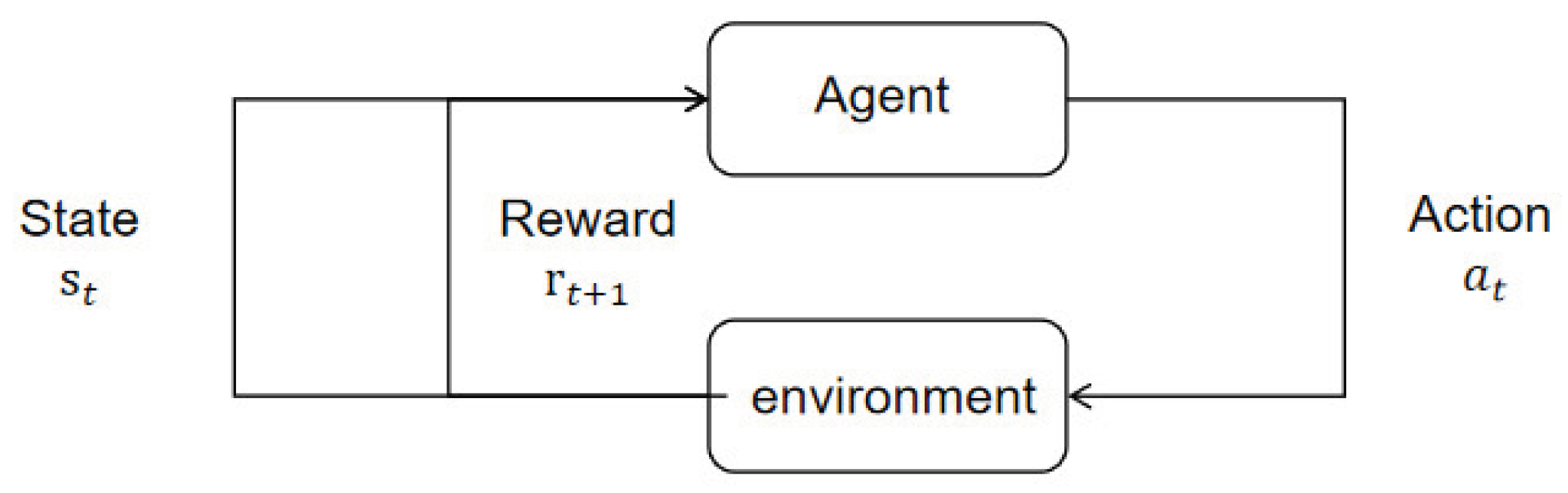
Reinforcement learning comprises two components: the agent and the environment. It involves the agent interacting with an uncertain external environment to maximize its cumulative reward through optimized action strategies. State, action, and reward are the three crucial elements of reinforcement learning: the state represents the environmental information observed by the agent; the action is the decision made by the agent based on the state, which can be discrete or continuous; the reward is the feedback provided by the environment in response to the agent’s actions, serving as an indicator of the current environment’s quality [10].

The process of an agent interacting with its environment is fundamentally a Markov decision process [11]. Each time an agent selects and executes an action based on the current environmental state, it receives corresponding rewards from the environment and transitions to the next state. This process is termed a Markov decision process, as illustrated in Figure 1. Also known as a Markov chain [12], a Markov decision process is a memoryless random sequence with Markovian properties. It can be represented by a quadruple (S, A, R, P), where:

S is the state space, representing the set of possible states perceived by the agent in the environment [14]. $s_t\in \mathrm{S}$denotes the state perceived by the agent in the environment at time t;

A is the action space, representing the set of actions the agent can perform.${\mathrm{a}}_{\mathrm{t}}\in \mathrm{A}$ denotes the action taken by the agent at time t;

R is the reward function, representing the corresponding reward fed back by the environment after the agent executes an action.${\mathrm{r}}_{\mathrm{t}}\in \mathrm{R}({\mathrm{s}}_{\mathrm{t}}，{\mathrm{a}}_{\mathrm{t}})$denotes the immediate reward obtained by the agent for executing action $a_t$ in state $s_t$;

P is the state transition probability, representing the probability that the agent transitions from the current state s to the next state s’ after executing action a at time t [15], expressed as

$$\mathrm{P}\left({\mathrm{s}}^{\mathrm{’}}|\mathrm{s},\mathrm{a}\right)=\mathrm{P}\left({\mathrm{s}}_{\mathrm{t}+1}={\mathrm{s}}^{\mathrm{’}}|{\mathrm{s}}_{\mathrm{t}}=\mathrm{s}，{\mathrm{a}}_{\mathrm{t}}=\mathrm{a}\right)$$

(13)

3.2. Q-Learning and Deep Q-Networks

Reinforcement learning can be categorized into value-based reinforcement learning algorithms and policy-based reinforcement learning algorithms based on the nature of the agent’s learning content [16]. Q-learning is a value-based reinforcement learning algorithm, belonging to the class of model-free reinforcement learning methods. It does not require prior knowledge of the environment’s specific model, learning solely through interaction with the environment. It is primarily used for agents to learn how to make decisions that maximize rewards during their interactions with the environment [17]. Q-learning defines a state value function, commonly referred to as the Q-function. It iteratively learns this Q-function by substituting observed data into the Bellman equation. The Bellman equation describes the update rule for the Q-value function and is the core of Q-learning. It is typically expressed as:

$${\mathrm{Q}}_{\mathrm{t}+1}\left({\mathrm{s}}_{\mathrm{t}},{\mathrm{a}}_{\mathrm{t}}\right)={\mathrm{Q}}_{\mathrm{t}}\left({\mathrm{s}}_{\mathrm{t}},{\mathrm{a}}_{\mathrm{t}}\right)+\mathsf{\alpha }\left[{\mathrm{r}}_{\mathrm{t}+1}+\mathsf{\gamma }\underset{{\mathrm{a}}^{\mathrm{’}}}{\max }\mathrm{Q}\left({\mathrm{s}}_{\mathrm{t}+1},{\mathrm{a}}^{\mathrm{\text{'}}}\right)-{\mathrm{Q}}_{\mathrm{t}}\left({\mathrm{s}}_{\mathrm{t}},{\mathrm{a}}_{\mathrm{t}}\right)\right]$$

(14)

where:

${\mathrm{Q}}_{\mathrm{t}}\left({\mathrm{s}}_{\mathrm{t}},{\mathrm{a}}_{\mathrm{t}}\right)$denotes the Q-value of action a taken in state s at time t;

α is the learning rate, controlling the trade-off between new and old estimates;

γ is the discount factor, representing the decay rate of future Q-values in the present, reflecting the importance of future rewards.

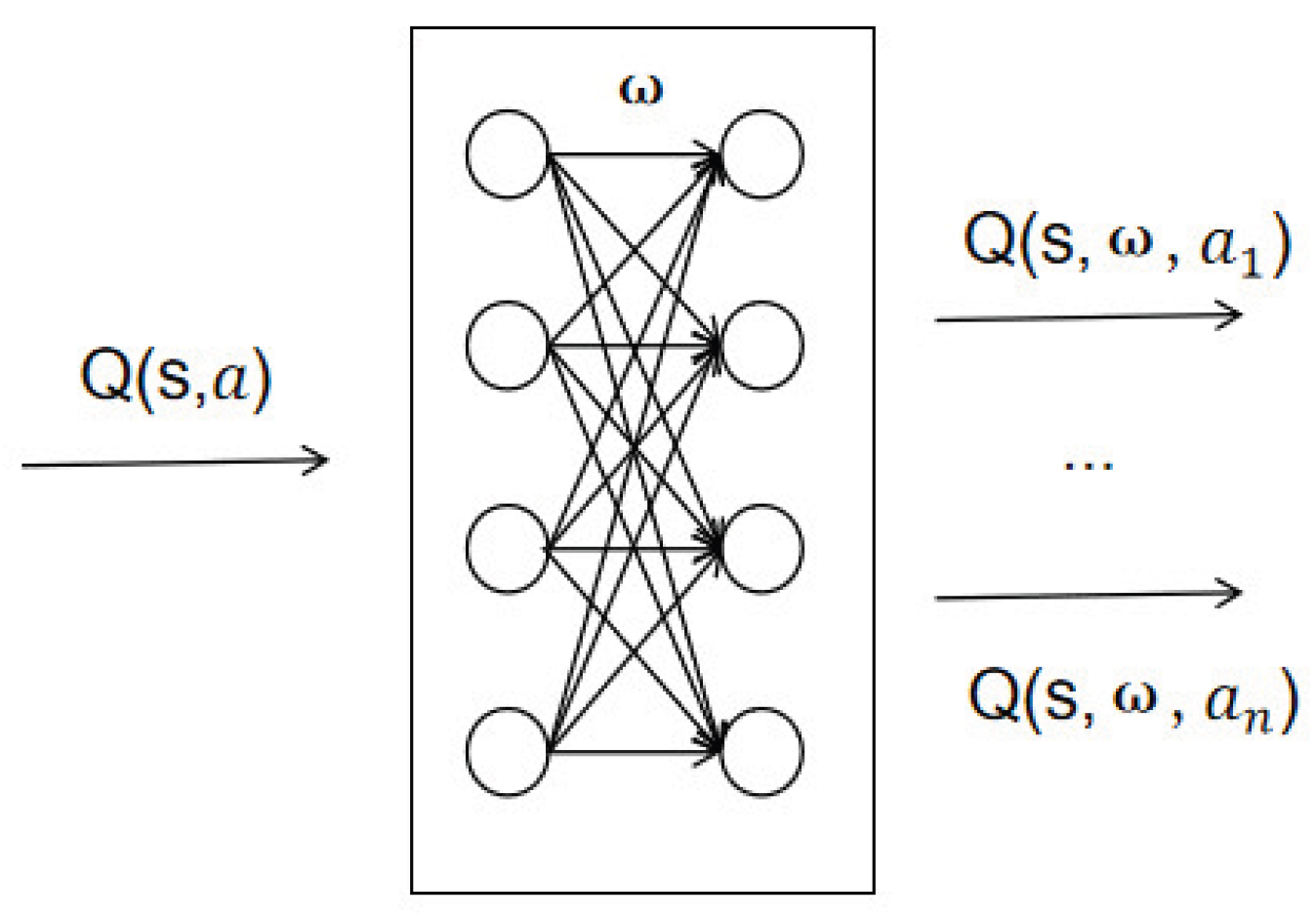
The Bellman equation clearly demonstrates how the current estimate, immediate reward, and maximum Q-value of the next state update the Q-function, proving that Q-learning can continuously approximate optimal action policies under this mechanism. However, due to the curse of dimensionality, traditional Q-learning algorithms struggle to solve large-scale MDP problems. To address this, value function approximation methods were developed. These methods approximate the value function Q using functions defined by parameters ω, with the computational process illustrated below. Deep neural networks represent one of the most commonly used function approximation methods in reinforcement learning [18].

$$\stackrel{\wedge }{Q}\left(\mathrm{s},a,\omega \right)\approx Q\left(\mathrm{s},a\right)$$

(15)

Deep reinforcement learning builds upon traditional reinforcement learning by utilizing deep neural networks to establish correspondences between state variables and action variables. Due to the powerful expressive capabilities of deep neural networks, deep reinforcement learning can handle more complex, real-world policy decision problems [19]. Deep Q-Network (DQN) is a representative deep reinforcement learning algorithm developed from Q-learning and deep neural networks. Compared to Q-learning, DQN primarily transforms the Q-function into a deep neural network through value function approximation methods [20], as illustrated in Figure 2.

3.3. Twin Delay Deep Deterministic Policy Gradient Algorithm

Deep Deterministic Policy Gradient (DDPG) evolved from the DQN algorithm, transcending the limitations of purely value-based or policy-based approaches. It represents a widely adopted actor-critic method that combines both, serving as a classic reinforcement learning algorithm for continuous control domains. Typically, it comprises a policy network and a value network [21]. However, like DQN, DDPG suffers from overestimation of Q-values, where the value network outputs Q-values higher than the actual action value. Additionally, training the Critic network and Actor simultaneously can lead to instability, and the policy’s direct output of deterministic actions during training may cause policy noise, trapping the algorithm in local optima.

To address these challenges, the TD3 algorithm emerged as an enhancement to DDPG. Building upon DDPG, TD3 introduces three key improvements targeting these three issues [22]:

To address the systematic overestimation of Q-values in DDPG’s Critic network, TD3 employs two independent Critic networks. These networks simultaneously learn by minimizing the mean squared error, targeting the same Q-value objective. The constructed target Q-value utilizes the smaller output from the two networks to reduce overestimation errors, preventing the policy from being misguided by inaccurate Q-value estimates during training. The target Q-value can be expressed as:

$${\mathrm{y}}_{\mathrm{t}}={\mathrm{r}}_{\mathrm{t}}+\gamma \min \left[Q_{{\theta }_1^{\text{'}}}\left(s_{t+1},a_{t+1}^{\text{'}},{\theta }_1^{\text{'}}\right),Q_{{\theta }_2^{\text{'}}}\left(s_{t+1},a_{t+1}^{\text{'}},{\theta }_2^{\text{'}}\right)\right]$$

(16)

In the equation, ${\mathsf{\theta }}_1^{\mathrm{\text{'}}}$ and ${\mathsf{\theta }}_2^{\mathrm{\text{'}}}$ represent the parameters of target value network 1 and target value network 2, respectively [23].

To avoid frequent updates of the Actor network causing policy instability and resulting in a vicious cycle of deterioration between the policy network and value network, the update frequency of the policy network should be lower than that of the value network. This ensures that the estimation error of the value network is reduced before the policy network is updated. TD3 updates the policy network and target network at a lower frequency while updating the value network more frequently, typically updating the actor network once after two critic network updates [10]. The loss functions $\mathrm{L}\left({\mathsf{\theta }}_1\right)$and $\mathrm{L}\left({\mathsf{\theta }}_2\right)$for training value networks 1 and 2, respectively, are constructed based on Equation 16 as follows:

$$\underset{{\theta }_1}{\min } L\left({\theta }_1\right)=E{\left[Q_{{\theta }_1}\left(s_t,a_{\mathrm{t}},{\theta }_1\right)-{\mathrm{y}}_{\mathrm{t}}\right]}^2$$

(17)

$$\underset{{\theta }_2}{\min } L\left({\theta }_2\right)=E{\left[Q_{{\theta }_2}\left(s_t,a_{\mathrm{t}},{\theta }_2\right)-{\mathrm{y}}_{\mathrm{t}}\right]}^2$$

(18)

Value Network 1 and Value Network 2 are updated using stochastic gradient descent, with the update formula being:

$${\theta }_{\mathrm{k}}\leftarrow {\theta }_{\mathrm{k}}-{\alpha }^{{\theta }_{\mathrm{k}}}{\nabla }_{{\theta }_{\mathrm{k}}}L\left({\theta }_{\mathrm{k}}\right),\mathrm{k}=1,2$$

(19)

In DDPG, the target policy directly outputs deterministic actions, making it prone to overfitting extreme actions. TD3 introduces truncated normal distribution noise to the target actions, thereby “smoothing” the actions. By estimating target Q-values using actions within a neighborhood of the target policy, TD3 smooths Q-value variations across different actions. This makes it harder for the policy to exploit Q-function errors, enhancing the algorithm’s robustness against noise and target value fluctuations. Target policy smoothing can be expressed as:

$$a_{\mathrm{t}+1}^{\text{'}}={\mu }^{{\varphi }^{\text{'}}}\left(s_{t+1}\right)+\epsilon ,\epsilon ~clip(N(0,\sigma ),-c,c)$$

(20)

In the equation, ε represents the small-variance policy noise following a normal distribution, c and -c denote the upper and lower noise clipping limits respectively to prevent excessive noise, and ${\mathsf{\phi }}^{\mathrm{\text{'}}}$ is the target policy network parameter.

4. TD3-Based Optimized Scheduling Method and Experiment

This paper employs the TD3 deep reinforcement learning algorithm for buoy system energy scheduling. Using a data-driven approach, an agent is trained to make rapid and accurate scheduling decisions based on real-time data, thereby achieving operational optimization of the buoy system [12].

4.1. Method

The buoy system’s energy management operates on a 24-hour scheduling cycle, dynamically allocating power output from the combined power supply unit and battery energy storage unit based on actual system conditions and load demands. Consequently, the control variables for the optimization problem focus on adjusting the power output of the generation unit at each scheduling time point.

4.1.1. State Space

For the buoy system model, the information provided by the environment to the agent typically includes renewable energy output, load, and the state of charge for electrical energy storage. Therefore, the state space of the buoy system model is defined as:

$$S=\left[P_{RE}^{\mathrm{t}},P_L^{\mathrm{t}},W_{\mathrm{B}}^{\mathrm{t}}\right]$$

(21)

In the formula: ${\mathrm{P}}_{\mathrm{R}\mathrm{E}}^{\mathrm{t}}$ denotes the power output of renewable energy during time period t, in kW; ${\mathrm{P}}_{\mathrm{L}}^{\mathrm{t}}$ denotes the load demand during time period t, in kW; ${\mathrm{W}}_{\mathrm{B}}^{\mathrm{t}}$ denotes the state of charge of electrical energy storage during time period t.

4.1.2. Action Space

Based on the control requirements of the buoy system, the action space is designed to reflect potential scheduling decisions, such as input adjustments for renewable energy and battery charging/discharging strategies. After observing the state information of the environment, the agent selects one or more actions from the action space according to its own policy set. The TD3 network can output three actions at once to achieve the purpose of scheduling control. The buoy system can be divided into power supply equipment and energy storage equipment. The action space is designed as follows:

$$A=\left[A_{\mathrm{RE}}^{\mathrm{t}},A_{\mathrm{Li}}^{\mathrm{t}},A_B^{\mathrm{t}}\right]$$

(22)

In the formula: ${\mathrm{A}}_{\mathrm{R}\mathrm{E}}^{\mathrm{t}}$ denotes the control action of renewable energy during time interval t; ${\mathrm{A}}_{\mathrm{L}\mathrm{i}}^{\mathrm{t}}$ denotes the control action of the lithium battery pack during time interval t; ${\mathrm{A}}_{\mathrm{B}}^{\mathrm{t}}$ denotes the control action of battery energy storage during time interval t.

4.1.3. Reward Function

The core objective of buoy system optimization is to ensure the safe and stable supply of electrical energy to meet system load demands, while simultaneously minimizing operational costs to the greatest extent possible. The reinforcement learning agent maximizes cumulative rewards to achieve the highest reward value; the buoy system must maintain supply-demand balance. When energy generation exceeds or falls short of demand, penalties should be applied to correct the agent’s actions [12]. The reward function is expressed as follows:

$$\mathrm{r}=-\left(C_{\mathrm{t}}+P_{\mathrm{pen}}^{\mathrm{t}}\right)/\delta$$

(23)

In the formula: ${\mathrm{C}}_{\mathrm{t}}$ is the objective function in the aforementioned buoy system cost model; ${\mathrm{P}}_{\mathrm{p}\mathrm{e}\mathrm{n}}^{\mathrm{t}}$ is the penalty term; δ is the scaling factor used to scale the reward. Scaling the reward helps maintain numerical stability and avoids extreme values in gradient estimation.

4.2. Experiment

This section demonstrates the application of the TD3 algorithm in solving the energy management optimization problem for a buoy system through specific numerical examples. It analyzes the economic optimization results under different energy configurations, illustrating the effectiveness of the TD3 algorithm.

When validating the buoy system scheduling method proposed in this paper, the buoy system described in Section 2.1 was selected as the research subject. The buoy system structure is shown in the figure, and the abbreviations and operating parameters of the experimental equipment are listed in Table 1.

For the power supply section of the buoy system, renewable energy sources include wind turbines and photovoltaic panels. The wind turbine has a maximum power output of 100W, while the photovoltaic system has a maximum power output of 150W. while the lithium battery pack has a maximum power output of 10W. The energy storage section features a battery capacity of 19.2kWh. During system operation, PV and WT will output power at their real-time maximum generation capacity, with lithium batteries and storage batteries coordinating power supply in real-time based on PV and WT generation conditions.

The TD3 algorithm was selected for optimization calculations in this experiment. The nonlinear programming results obtained for all variables—including auroral irradiance, wind speed, and buoy load at each time point—represent the optimal scheduling strategy under ideal conditions. All Arctic field data used in this experiment—including irradiance, wind speed, and temperature—were sourced from the NSF Data Center. The load represents the total power consumption of all buoy sensors. The dataset comprises 180 days of data with a 1-hour resolution, including sampling timestamps for Arctic field irradiance, wind speed, and temperature. Simulation parameters are detailed in Table 2.

4.3. Results

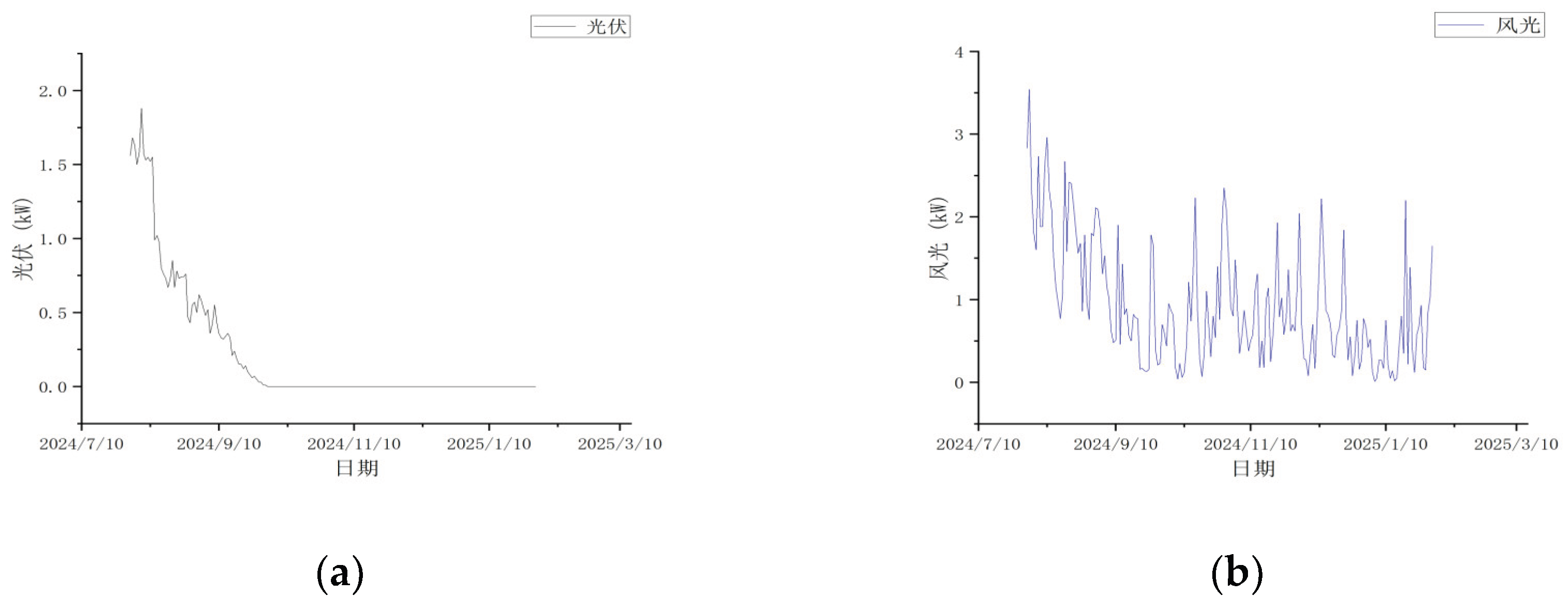
This experimental case study was conducted in the Arctic from August 2024 to January 2025. as shown in Figure 3. By adjusting the discharge power of lithium batteries and the charging/discharging power of battery storage systems under varying on-site temperatures in the Arctic, the power supply costs for the lithium battery pack over the 180-day period were optimized.

When training the TD3 algorithm, each component of the state variables must be normalized before being fed into the TD3 critic network for training. Considering that the control objective in this paper is to minimize power supply costs, a 2x amplification factor is applied to the power deviation state variable during training to enhance the influence of system power balance on the control objective. The training time step is set to 300 seconds, resulting in a training cycle of 200 steps.

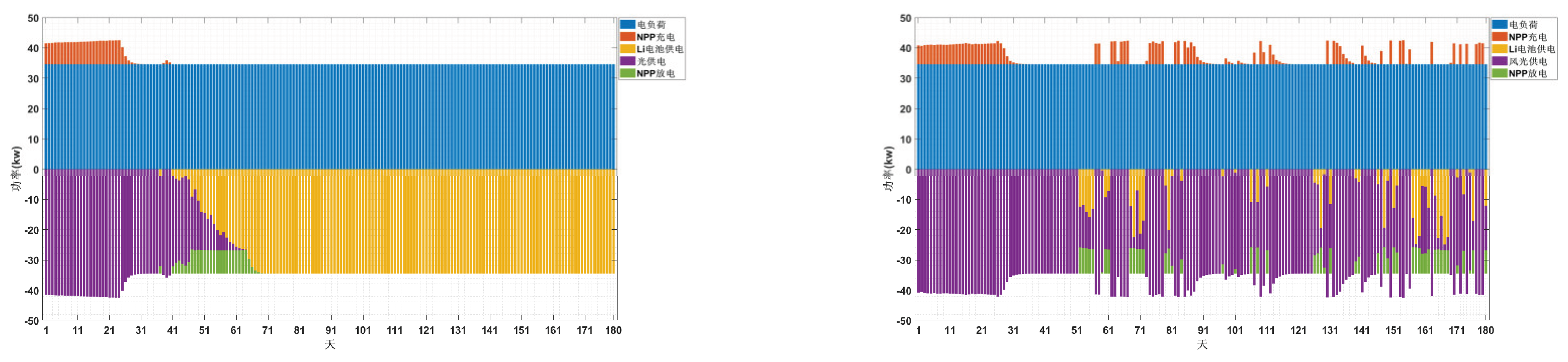
Figure 4 illustrates the power variation trends of PV, lithium batteries, energy storage, and loads, as well as PV, wind turbines, lithium batteries, energy storage, and loads over a six-month period (180 days). The horizontal axis represents time in days, while the vertical axis denotes power in kW. The PV, wind turbine, temperature, and load curves are predefined external data. The energy storage power is the strategy output from the neural network trained by TD3, and the power supply from the lithium battery bank is then determined based on power balance.

Referring to Figure 5, the energy storage charging and discharging strategy derived from the TD3 algorithm is as follows: prior to deployment in the Arctic, solar and wind power generation remain inactive while the energy storage system discharges until its capacity reaches the lower limit. Subsequently, solar and wind power generation commence, initiating the charging of the energy storage system. Excess power generated by solar and wind sources beyond the buoy system’s load requirements is stored. After 20-30 days of continuous charging until full capacity, the energy storage system ceases operation. Subsequently, any power generation from photovoltaic and wind sources that exceeds the maximum storage capacity of the batteries is discarded. During low-output periods for Arctic photovoltaic and wind power, the batteries discharge in coordination with the lithium batteries to supply the buoy system’s load. The batteries recharge during peak photovoltaic and wind generation periods.

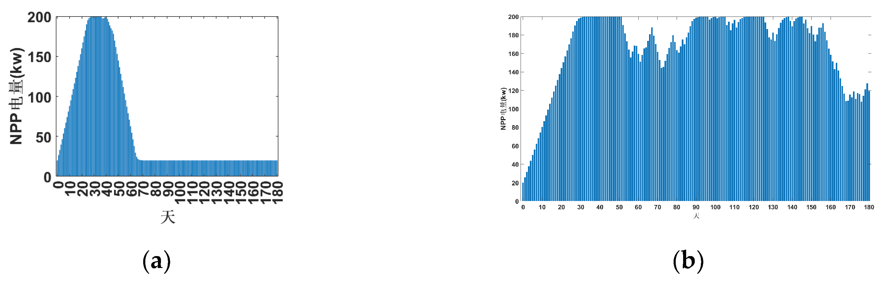
The experiment compared two energy configurations using the TD3 algorithm: one combining photovoltaic power with lithium batteries and lead-acid batteries, and another adding wind power to supply the buoy system. The control strategy effectively utilizes abundant solar energy during Arctic midnight sun periods and wind energy during strong winds to meet the buoy system’s load and store excess power. This reduces lithium battery usage costs while ensuring the buoy system’s continuous operation for over six months. Buoy deployment typically occurs during the Arctic summer months of August-September, when the Arctic daylight period lasts only about 60 days. Compared to systems powered solely by photovoltaics, integrating wind power enables the buoy system to continue supplementing renewable energy supply even after the Arctic enters its polar night, effectively ensuring prolonged continuous operation. According to TD3 algorithm calculations, a photovoltaic-only buoy system requires lithium batteries to generate 61.44 kWh of electricity. In contrast, a buoy system incorporating wind turbine power generation requires only 7.685 kWh from lithium batteries. This validates the economic viability of reducing lithium battery costs by adding wind turbines to buoy systems and confirms the feasibility of ensuring system operation.

5. Conclusions

This paper addresses the energy management challenge for Arctic space environment monitoring buoys by proposing a deep reinforcement learning method based on the TD3 algorithm. Simulation experiments validate its effectiveness in optimizing lithium battery power supply costs and ensuring long-term operational reliability. Experimental results demonstrate that over an 180-day Arctic operational cycle, the buoy system integrated with wind turbine power supply significantly reduces energy costs compared to a standalone photovoltaic system while maintaining monitoring continuity. Furthermore, the TD3 algorithm enhances training efficiency and policy robustness through dynamic adjustment and normalization of the power deviation state variable.

However, this study has limitations. For instance, it did not verify whether the TD3 algorithm outperforms other algorithms in calculating buoy system economics. Actual buoy operations may encounter more complex extreme weather events like blizzards, which the current model does not fully account for. The long-term impact of battery life degradation requires further modeling and analysis. Real-time performance of the algorithm on edge devices still needs optimization.

Future research will integrate multi-agent reinforcement learning to optimize collaborative energy scheduling among multiple buoys, incorporate transfer learning to adapt energy management to diverse polar environments, and develop lightweight DRL algorithms to enhance real-time edge computing performance. This study offers novel insights for energy management in intelligent polar observation equipment while establishing a theoretical foundation for renewable energy utilization and energy storage optimization in extreme environments.

References

- Zhang, Chuanqiang. Structural Design and Experimental Study of a Miniature Wave Energy Piezoelectric Power Generation Device [D]. Zhejiang Ocean University, 2023. [CrossRef]
- Tang Hongjian. Research on AUV Path Planning Methods Based on Deep Reinforcement Learning [D]. Harbin Engineering University, 2024. [CrossRef]
- Zhang Qiang, Wen Wen, Zhou Xiaodong, et al. Research on Intelligent Planning Methods for Robotic Arms Based on an Improved TD3 Algorithm [J]. Journal of Intelligent Science and Technology, 2022, 4(02): 223-232.
- Li Xiaowei, Ma Keyan. Band-Specific Study on the Irradiation Effects of Laser on Photovoltaic Cells [J]. Optoelectronic Technology, 2018, 38(03): 184-189. [CrossRef]
-
He Bo. Research on Health Status Evaluation and Prediction of Wind Turbines Based on Data Mining [D]; Guizhou University, 2023.
- Liu Junfeng, Chen Jianlong, Wang Xiaosheng, et al. Research on Energy Management and Optimization Strategies for Microgrids Based on Deep Reinforcement Learning [J]. Power System Technology 2020, 44(10), 3794–3803. [CrossRef]
- Zhou Yin. Research on the Joint Optimization Method for Generation, Load, and Storage in Industrial Parks [J]. Automation Applications 2021, (12), 134–138. [CrossRef]
Liu Di. Research on an Integrated Method for Micro-Energy Network Operation Optimization and Planning [D]; Beijing Jiaotong University, 2019.
- Zeng Lei, Ding Quan, Chen Xiaoyu, et al. Deep Reinforcement Learning-Based Optimization Method for Microgrid Operation [J]. Zhejiang Electric Power 2025, 44(06), 31–40. [CrossRef]
- Chen Xiaofang. Research on Intelligent Optimization Operation of Integrated Energy Systems Based on Deep Reinforcement Learning [D]. South China University of Technology, 2023. [CrossRef]
- Hao Xiuzhao. Research on Improvement of Motion Coordination Algorithm Based on Reinforcement Learning in Specific Road Network Environments [D]. In Beijing Jiaotong University; 2020. [CrossRef]
- Zeng Lei. Research on Reinforcement Learning-Based Task Scheduling Optimization for Cloud Data Centers [D]. In Nanjing University of Information Science and Technology; 2023.
- Wu, Y. R., & Zhao, H. S. (2010). Wind turbine maintenance optimization based on Markov decision processes [C]. In Proceedings of the 26th Annual Conference on Power System and Its Automation of Chinese Universities and the 2010 Annual Meeting of the Power System Committee of the Chinese Society for Electrical Engineering. 2010-10-01.
- Li Peng, Jiang Lei, Wang Jiahao, et al. Dual-timescale reactive power and voltage optimization for new energy distribution networks based on deep reinforcement learning [J]. Transactions of the Chinese Society for Electrical Engineering 2023, 43(16), 6255–6266. [CrossRef]
- Zhou Bin, Guo Yan, Li Ning, et al. Path Planning for Unmanned Aerial Vehicles Based on Guided Reinforcement Q-Learning [J]. Acta Aeronautica et Astronautica Sinica 2021, 42(09), 506–513.
- Rao Chao. Research on Deep Reinforcement Learning Recommendation Algorithms for Interactive Recommendation Systems [D]. In Huazhong University of Science and Technology; 2021. [CrossRef]
Wang Weiqiang. Research on Robot Autonomous Navigation Based on Safe Reinforcement Learning in Unknown Dynamic Environments [D]; Yancheng Institute of Technology, 2023.
- Chen Jianlong. Research on Energy Management Strategies for Microgrids Based on Deep Reinforcement Learning [D]. South China University of Technology, 2020. Author 1, A.B.; Author 2, C.D. Title of the article. Abbreviated Journal Name Year, Volume, page range. [CrossRef]
- Liang Hong, Li Hongxin, Zhang Huaying, et al. Research on Control Strategy for Microgrid Energy Storage Systems Based on Deep Reinforcement Learning [J]. Power System Technology 2021, 45(10), 3869–3877. [CrossRef]
- Zhang, Z. Research on Bus Signal Priority Control Based on Deep Reinforcement Learning [D]. In Lanzhou Jiaotong University; 2024. [Google Scholar] [CrossRef]
- Zhao Tianliang, Zhang Xiaojun, Zhang Minglu, et al. Research on Autonomous Driving Path Planning Based on Deep Reinforcement Learning [J]. Journal of Hebei University of Technology 2024, 53(04), 21–30. [CrossRef]
- Zhong Yadong. Research on Robot Plugging Algorithm Integrating Transfer Reinforcement Learning and Neighborhood Generalization [D]. In Wuhan University of Technology; 2023. [CrossRef]
- Zhou Xiang, Wang Jiye, Chen Sheng, et al. Review of Microgrid Optimization Operation Based on Deep Reinforcement Learning [J]. Global Energy Interconnection, 2023, 6(03): 240-257. Author 1, A.; Author 2, B. Title of the chapter. In Book Title, 2nd ed.; Editor 1, A., Editor 2, B., Eds.; Publisher: Publisher Location, Country, 2007; Volume 3, pp. 154–196. [CrossRef]