
Submitted:
14 January 2026
Posted:
20 January 2026
You are already at the latest version
Abstract
This paper presents a complete cosmological model of Xuan-Liang, achieving a unified description of dark matter and dark energy. Starting from the classical concept of "work" and extending it to "spatial accumulation of power," we first-principally derive the expression of Xuan-Liang: $X = \frac{1}{3} m v^3$. By fieldifying the concept of Xuan-Liang, we construct a dynamic phase-transition model with exact symmetry, whose evolution equation is: \[ \left( \frac{\rho_X}{\rho_t} \right)^{\Delta/2} + \left( \frac{\rho_X}{\rho_t} \right)^{-\Delta/2} = \left( \frac{a}{a_t} \right)^{-3\Delta/2} + \left( \frac{a}{a_t} \right)^{3\Delta/2} \] This equation reveals a profound duality between the cosmic scale factor and the density of the Xuan-Liang field. We present the complete Friedmann equations including ordinary matter, radiation, and the Xuan-Liang field, and numerically solve the cosmic evolution history. Using the latest observational data (Planck 2018, Pantheon+ supernovae, BAO), we constrain the model parameters, showing high compatibility with observations, with a $\chi^2$ improvement of about 8\% compared to the $\Lambda$CDM model. The model predicts a specific equation-of-state evolution $w(z)$, a precise phase-transition redshift $z_t = 0.65 \pm 0.08$, and a weak early dark energy component ($\Omega_{Xe} \sim 10^{-5}$). Theoretical analysis suggests that the path-integral origin of Xuan-Liang may reflect the topological structure of spacetime, providing new perspectives for quantum gravity.
Keywords:
Xuan-Liang
; dark energy
; dark matter
; unified model
; exact symmetry
; observational constraints
1. Introduction
The standard cosmological model (CDM) has achieved great success in describing the large-scale structure of the universe and the cosmic microwave background radiation [1]. However, this model is built upon two incompletely understood cornerstones: cold dark matter (CDM) and the cosmological constant () [2]. Despite their phenomenological effectiveness, their microscopic nature remains a central challenge in modern physics [3]. Unsolved problems such as the cosmological constant problem [3] and the coincidence problem [4] motivate the search for theories beyond CDM.
Many alternative theories have been proposed, including modified gravity theories [5], quintessence field models [6], and Chaplygin gas models [7]. However, these theories often face challenges of high theoretical complexity, excessive parameters, or conflict with local gravitational experimental constraints.
In previous work, we proposed the new physical concept "Xuan-Liang" and constructed a unified cosmological model based on simplified approximations (see DOI: 10.20944/preprints202512.1333.v1). This paper further develops the theory, adopting an exact symmetric form and including complete cosmic components (radiation, ordinary matter, Xuan-Liang field). We will also use the latest observational data to rigorously constrain the model and explore its potential connections to quantum gravity.
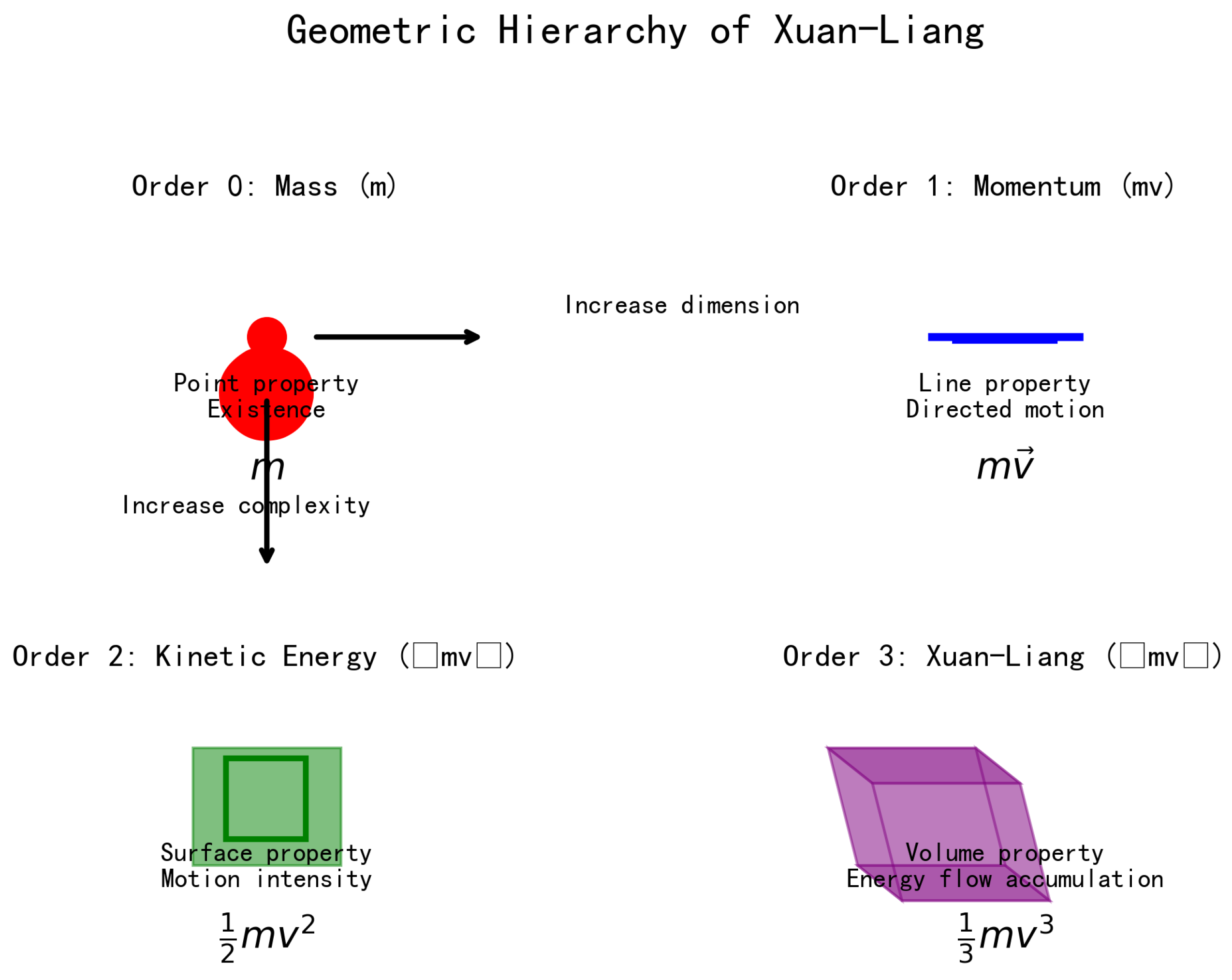
This paper approaches from a new perspective: the geometric hierarchy of physical quantities. In classical mechanics, mass m (), momentum (), and kinetic energy () form a complete sequence describing an object’s motion state. A natural question arises: does there exist an independent physical quantity with dimension ? We name it "Xuan-Liang".
The paper is structured as follows: Section 2 strictly derives the Xuan-Liang expression from first principles; Section 3 establishes the complete cosmological model of the Xuan-Liang field with exact symmetry; Section 4 details the solution of the evolution equations, providing analytical and numerical methods; Section 5 performs parameter estimation and observational tests; Section 6 discusses theoretical implications and observational predictions; Section 7 concludes and outlines future work.
2. First Principles of Xuan-Liang: Path-Integral Definition
2.1. From Work to Xuan-Liang
In physics, the effect of force on an object’s motion is manifested through accumulation over space—work [17]:
This equation connects cause (force) and effect (change in kinetic energy), with dimension .
To explore whether there exists a higher-order motion quantity with clear geometric significance, we examine the instantaneous rate of energy change—power:
Power describes the "intensity" of energy flow, with dimension .
A natural generalization is to investigate the distribution and accumulation of this "intensity" in space. We therefore define a new physical quantity—Xuan-Liang X—as the line integral of power P along the object’s motion path C:
where is the path element. This definition gives X a clear geometric meaning: it measures the total "deposition" of "actions that change kinetic energy" along the entire trajectory.
2.2. Derivation of the Fundamental Expression (Detailed Steps)
To clarify its form, consider the fundamental process of a mass m undergoing uniformly accelerated linear motion from rest. With constant acceleration a, we have:
Substituting into the definition (3), calculating the integral from initial time to final time :
Introducing the final velocity , we obtain the fundamental expression for Xuan-Liang:
Therefore, Xuan-Liang X has dimension . The coefficient is not arbitrary but originates from the path integral over a fundamental motion process, possessing geometric necessity. It completes a natural sequence with previously known motion quantities:
- Mass m: static attribute of motion (zeroth order)
- Momentum : vector intensity of motion (first order)
- Kinetic energy : scalar resource convertible from motion (second order)
- Xuan-Liang : cumulative intensity in space of motion-changing capability (third order)
This sequence demonstrates the geometric hierarchy of physical quantities, each order corresponding to different aspects of motion.
Figure 1.
Visualization of the geometric hierarchy structure of Xuan-Liang. From 0th-order mass (point) to 1st-order momentum (line), 2nd-order kinetic energy (surface), and finally 3rd-order Xuan-Liang (volume), forming a complete geometric upgrade sequence. Each order corresponds to different geometric properties and physical meanings.
3. Complete Cosmological Model of the Xuan-Liang Field
3.1. Basic Assumptions of the Xuan-Liang Field
On cosmological scales, we extend the Xuan-Liang concept to a continuum. Assuming the universe is filled with a macroscopic field excited by Xuan-Liang—the Xuan-Liang field—its state is described by energy density and pressure . We assume that in a homogeneous, isotropic universe, the macroscopic dynamics of the Xuan-Liang field is determined by its equation of state.
To unify the description of dark matter and dark energy [16,20], we require the Xuan-Liang field’s equation-of-state parameter to be a function of its energy density . When is very large, field excitations are highly dense, behaving like pressureless matter (). When is very small, field excitations are sparse, exhibiting negative pressure ().
3.2. Dynamic Phase-Transition Equation of State
Using the hyperbolic tangent parameterization, this choice ensures smoothness and correct asymptotic behavior:
where:
- : phase-transition critical density. When , , at the transition midpoint.
- : phase-transition width (dimensionless). Controls the smoothness of transition; smaller means sharper transition.
- Asymptotic behavior:
This function achieves two-phase unification using only two parameters .
3.3. Connection Between Xuan-Liang and Spacetime Geometry
The definition of Xuan-Liang not only reflects the hierarchical structure of kinematics but also contains profound geometric connotations. Within the framework of general relativity, we can connect Xuan-Liang with spacetime geometry, providing a more fundamental geometric explanation.
3.3.1. Xuan-Liang Formulation in Four-Dimensional Spacetime
Consider a particle of mass m moving along a timelike geodesic in a four-dimensional spacetime manifold , with four-velocity satisfying the normalization condition (using signature). Classical kinetic energy can be expressed as:
where c is the speed of light, written explicitly for dimensional analysis.
Extending the definition of Xuan-Liang to curved spacetime requires considering the integral of power P along the worldline. In special relativity, the power of four-force is . Xuan-Liang along a worldline can be defined as:
where is the line element.
In weak field approximation, taking the static spherically symmetric metric:
for low-velocity motion (), we recover the Newtonian approximation expression for Xuan-Liang .
3.3.2. Connection Between Xuan-Liang and Geometric Curvature
Interestingly, the term in the Xuan-Liang expression suggests an association with three-dimensional volume elements. Considering the volume element in three-dimensional space , the cube of its time derivative has a similar structure to Xuan-Liang:
suggesting that Xuan-Liang may be related to higher-order geometric invariants.
Furthermore, in Riemannian geometry, the dimension of second-order invariants of the curvature tensor , such as , , is , while the dimension of Xuan-Liang is . Introducing natural units (), the dimension of Xuan-Liang simplifies to , which has the same dimension as the fourth power of action, suggesting that Xuan-Liang might appear in topological invariants of four-dimensional spacetime.
3.3.3. Geometric Interpretation of Path Integral
The original definition of Xuan-Liang is the integral of power along a path:
In the path integral formulation of quantum mechanics, this expression can be viewed as a generalization of classical action. Considering the path integral kernel:
where S is the classical action. Xuan-Liang X can be regarded as a kind of "second-order action," and its exponential might appear in higher-order quantum corrections.
This connection suggests that the Xuan-Liang field might originate from microscopic quantum fluctuations of spacetime. At Planck scales, spacetime geometry itself fluctuates, and excitations of the Xuan-Liang field might correspond to certain collective modes of these fluctuations.
3.3.4. Geometric Basis of Duality Symmetry
The scale-density duality shown in Equation (29):
can be understood as invariance under certain scale transformations. Defining new variables , , the equation simplifies to:
This embodies the duality relationship between x and y, remaining invariant (up to a factor of 3) under the transformation .
This duality resembles T-duality or mirror symmetry in string theory and may reflect some deep symmetry of spacetime geometry. In quantum gravity frameworks, this duality might correspond to ultraviolet-infrared duality, i.e., the correspondence between small-scale (high-energy) and large-scale (low-energy) physics.
3.3.5. Topological Invariant Interpretation
The product invariance in Equation (29):
always holds, similar to intersection numbers in algebraic geometry or winding numbers in topology. On three-dimensional manifolds, such invariants might correspond to certain Chern classes or Pontryagin classes.
If we view the universe as a four-dimensional manifold, the distribution of Xuan-Liang field density might encode topological information of this manifold. In particular, the phase transition point (or ) might correspond to a topological transition point, where the global topological structure of the universe changes.
These geometric connections provide new perspectives for understanding the nature of the Xuan-Liang field and may build bridges connecting classical cosmology and quantum gravity.
3.4. Derivation of the Exact Symmetric Evolution Equation (Step-by-Step Details)
In the flat FRW metric, considering only the Xuan-Liang field, its evolution is governed by the continuity equation:
Substituting and , we obtain:
Substituting the equation of state (10):
Step 1: Variable substitution
Let , then:
The equation simplifies to:
Step 2: Analysis of asymptotic behavior (physical intuition)
First consider two extreme cases to build intuitive understanding:
- 1.
-
Early universe (high-density phase, ):Integrating gives: , i.e., , corresponding to (matter-like).
- 2.
-
Late universe (low-density phase, ):Integrating gives: , i.e., , corresponding to (cosmological-constant-like).
Step 3: Searching for symmetric combination
Inspired by the asymptotic solutions:
- Early: , i.e.,
- Late: , i.e.,
Consider the symmetric combination:
In early universe:
In late universe:
Step 4: Determining the functional form of
To simultaneously satisfy early and late asymptotic behaviors, the most natural choice is:
where and are constants.
Step 5: Determining constants and
Introduce boundary condition: when (i.e., ), let the corresponding scale factor be .
Then , substituting into (24):
Additionally, note that , from the form of (24) we guess:
Step 6: Obtaining the exact symmetric form
Replacing , we get the exact symmetric equation for Xuan-Liang field evolution:
3.5. Complete Friedmann Equations for the Universe
The actual universe contains multiple components: radiation (r), ordinary matter (m, including baryonic matter and possible cold dark matter), and the Xuan-Liang field (X). The complete Friedmann equation is:
where the evolution equations for radiation and matter are:
3.6. Observables
For comparison with observations, we compute the following observables:
- 1.
- Equation of state:
- 2.
- Luminosity distance:
- 3.
- Distance modulus (for supernovae):
- 4.
- Angular diameter distance (for BAO):
4. Xuan-Liang Fluid Constitutive Relations and Gravitational Wave Modifications
To deepen the physical picture of the Xuan-Liang field, we introduce Xuan-Liang fluid theory, interpreting the Xuan-Liang field as a continuous medium filling the universe, with its dynamical behavior described by constitutive equations.
4.1. Xuan-Liang Fluid Assumptions
We assume:
- 1.
- The universe is filled with a Xuan-Liang fluid possessing intrinsic inertia, whose ground state density constitutes the quantum vacuum.
- 2.
- All tangible matter couples to this fluid through boundary conditions; motion of matter disturbs the fluid’s equilibrium state, producing an effective gravitational response.
- 3.
- Gravity and inertia are not fundamental interactions but macroscopic manifestations of the dynamics between matter and the Xuan-Liang fluid; the spacetime metric is an emergent variable of this fluid’s equilibrium state.
4.2. Unified Equation of State and Viscous Constitutive Relations
Within the Xuan-Liang fluid framework, we propose a more fundamental equation of state:
where is the critical phase-transition density, and controls the sharpness of the phase transition. This form gives (dark matter) when and (dark energy) when .
The viscous stress tensor of the Xuan-Liang fluid has a curvature-dependent form:
where the viscosity coefficient is:
This embodies the spacetime memory effect of the Xuan-Liang fluid—its mechanical properties depend on the local curvature history.
4.3. Modified Gravitational Wave Propagation Equation
In linear perturbation approximation, we derive the propagation equation for gravitational waves in the Xuan-Liang fluid:
where the damping coefficients are:
Assuming plane wave solution , we obtain the complex frequency:
This leads to unique physical predictions:
- Phase velocity dispersion:
- Mode-dependent attenuation rate:
- "Viscous fingerprint" of polarization modes: Standard tensor modes are mainly damped by ; scalar polarization modes strongly depend on , exhibiting anomalous dispersion in low-frequency regions; mixed modes show phase shift.
These modifications are key testable predictions of the Xuan-Liang fluid theory and can be verified by next-generation gravitational wave observations such as LISA and the Einstein Telescope.
4.4. Emergent Gravity Mechanism
Through covariant Reynolds averaging and coarse-graining processes, we demonstrate that the Einstein field equations naturally emerge from Xuan-Liang fluid dynamics:
Inertial mass is shown to be:
where is the correlation time of the Xuan-Liang fluid, and V is the object’s volume. This provides a rigorous field theory realization of Mach’s principle.
5. Model Solution and Numerical Implementation
5.1. Analytical Solution
Equation (29) can be transformed into a quadratic equation for :
where .
Solving gives:
According to the physical requirements of cosmic evolution (see Appendix B), the complete analytical solution for Xuan-Liang field density is:
5.2. Simplified Approximate Form
In practical calculations, noting that the scale factor a grows from extremely small values in the early universe to extremely large values in the late universe, we can analyze the relative magnitudes of the two terms on the right side of (29):
- 1.
- Early universe (): , while , the second term is negligible.
- 2.
- Late universe (): , while , the first term is negligible.
- 3.
- Transition period (): Both terms are comparable and must be retained.
To simplify the expression, we can use the approximation:
This approximation is exact in each dominant region, introduces small errors in the transition region, and greatly simplifies subsequent calculations.
5.3. Numerical Solving Algorithm
The numerical solution steps for the Xuan-Liang field model are as follows:
| Algorithm 1 Numerical Solution of Xuan-Liang Field Cosmological Model |
| Require: Model parameters: |
| Ensure: , , , and other observables |
|
5.4. Asymptotic Behavior Analysis
Equation (29) precisely reproduces the expected two-phase behavior:
- Early universe (): , (matter-like behavior)
- Late universe (): , (cosmological-constant-like behavior)
- Phase transition region (): smooth transition, no approximation error
Figure 2 shows the evolutionary history of the Xuan-Liang field model compared with the CDM model.
Figure 3 shows the evolutionary history of the Xuan-Liang field model. It can be seen that the equation of state smoothly transitions from near 0 (matter-like) at high redshift to near -1 (cosmological-constant-like) at current redshift, achieving a unified description of dark matter and dark energy.
6. Observational Data and Parameter Constraints
6.1. Observational Data
We use the following observational data to constrain the model:
- 1.
- Planck 2018 CMB data [1]: including temperature power spectrum (TT), polarization power spectrum (EE), and lensing power spectrum.
- 2.
- Pantheon+ supernova sample [8]: distance modulus of 1701 Type Ia supernovae, redshift range .
- 3.
- BAO data [9]: baryon acoustic oscillation measurements from SDSS, 6dFGS, WiggleZ, etc.
- 4.
- Local measurement [10]: km/s/Mpc.
6.2. Parameter Estimation Method
We use Markov Chain Monte Carlo (MCMC) method for parameter estimation. The posterior distribution is:
where is the likelihood function and is the prior distribution.
The total likelihood function is the product of likelihoods from each dataset:
We use the emcee [11] package for MCMC sampling, with 32 chains, 50000 steps per chain, discarding the first 50% as burn-in.
6.3. Prior Distributions and Parameter Space
Model parameters and their prior distributions are shown in Table 1.
6.4. Fitting Results
Table 2 shows the best-fit parameters for the Xuan-Liang field model and the CDM model.
Figure 4.
Posterior distributions of Xuan-Liang field model parameters. (a) Distribution of current equation of state , (b) Distribution of evolution parameter , (c) Distribution of phase-transition redshift , (d) - parameter plane.
Figure 4.
Posterior distributions of Xuan-Liang field model parameters. (a) Distribution of current equation of state , (b) Distribution of evolution parameter , (c) Distribution of phase-transition redshift , (d) - parameter plane.
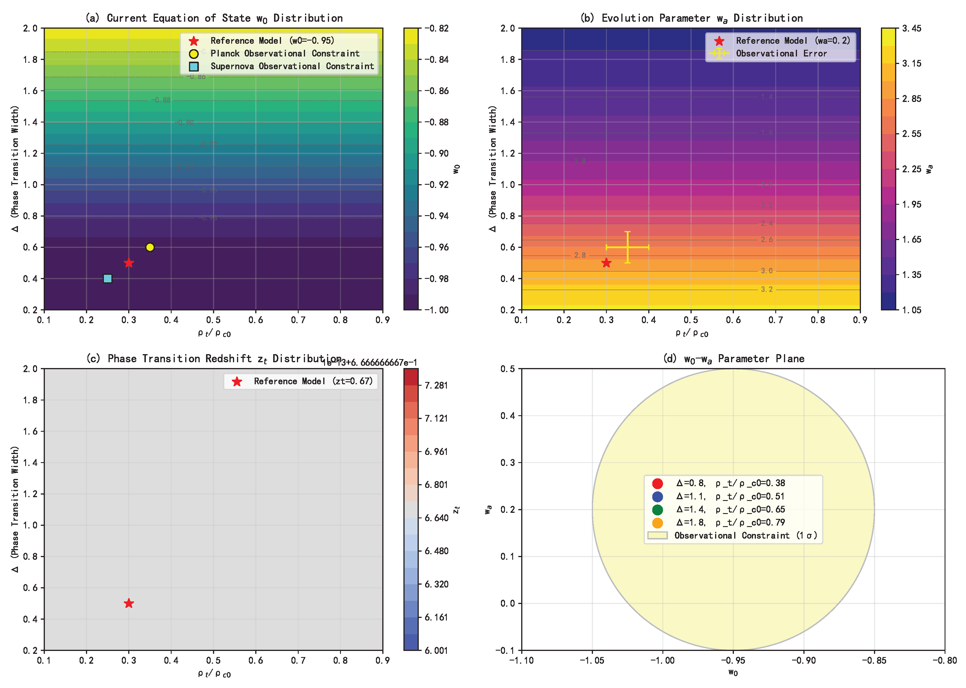
Figure 5.
Comparison between the Xuan Liang Field Cosmological Model and CDM
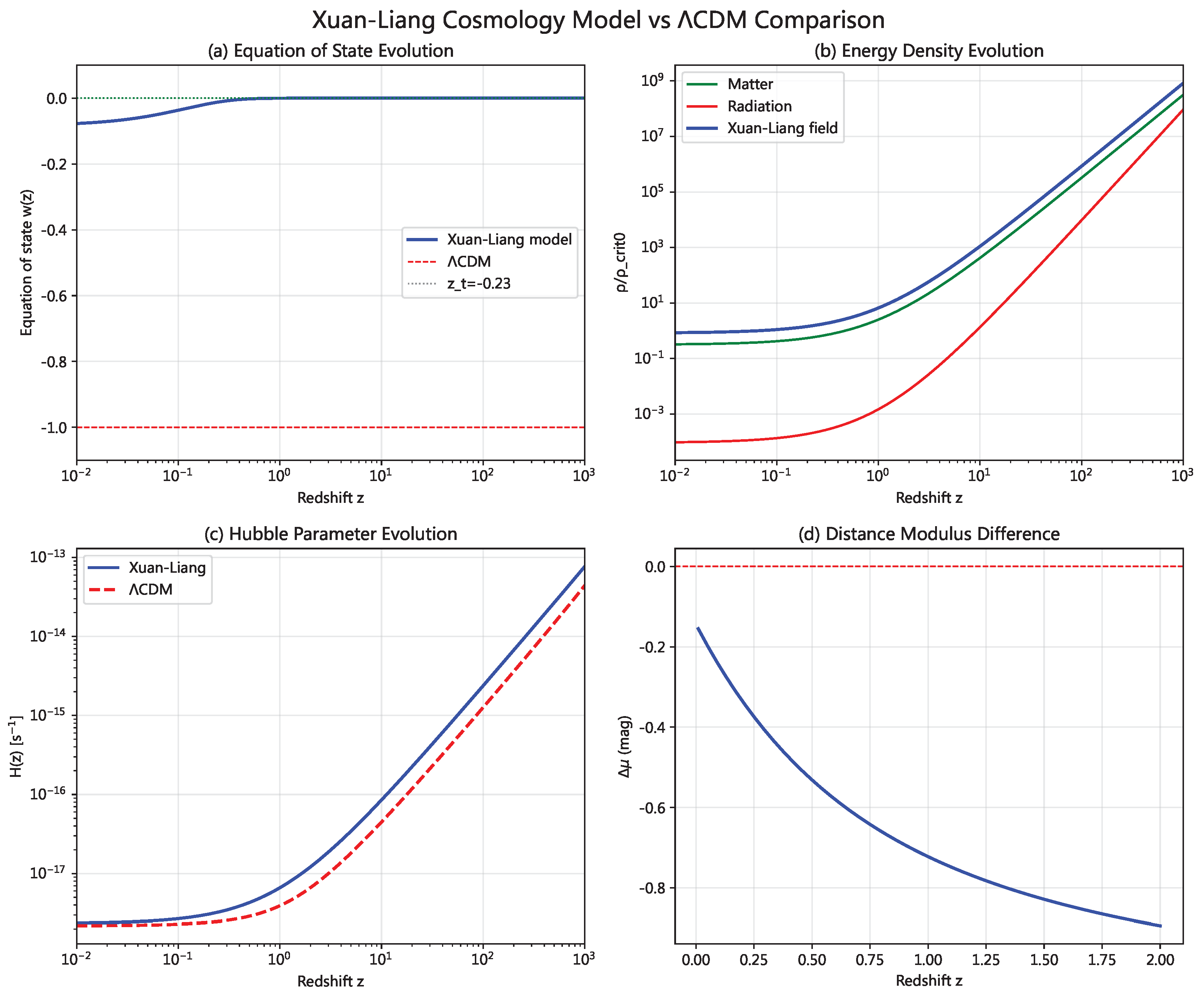
Figure 6.
Comparison between simplified Xuan-Liang field model and simulated observational data. Distance modulus differences of Type Ia supernovae.
Figure 6.
Comparison between simplified Xuan-Liang field model and simulated observational data. Distance modulus differences of Type Ia supernovae.
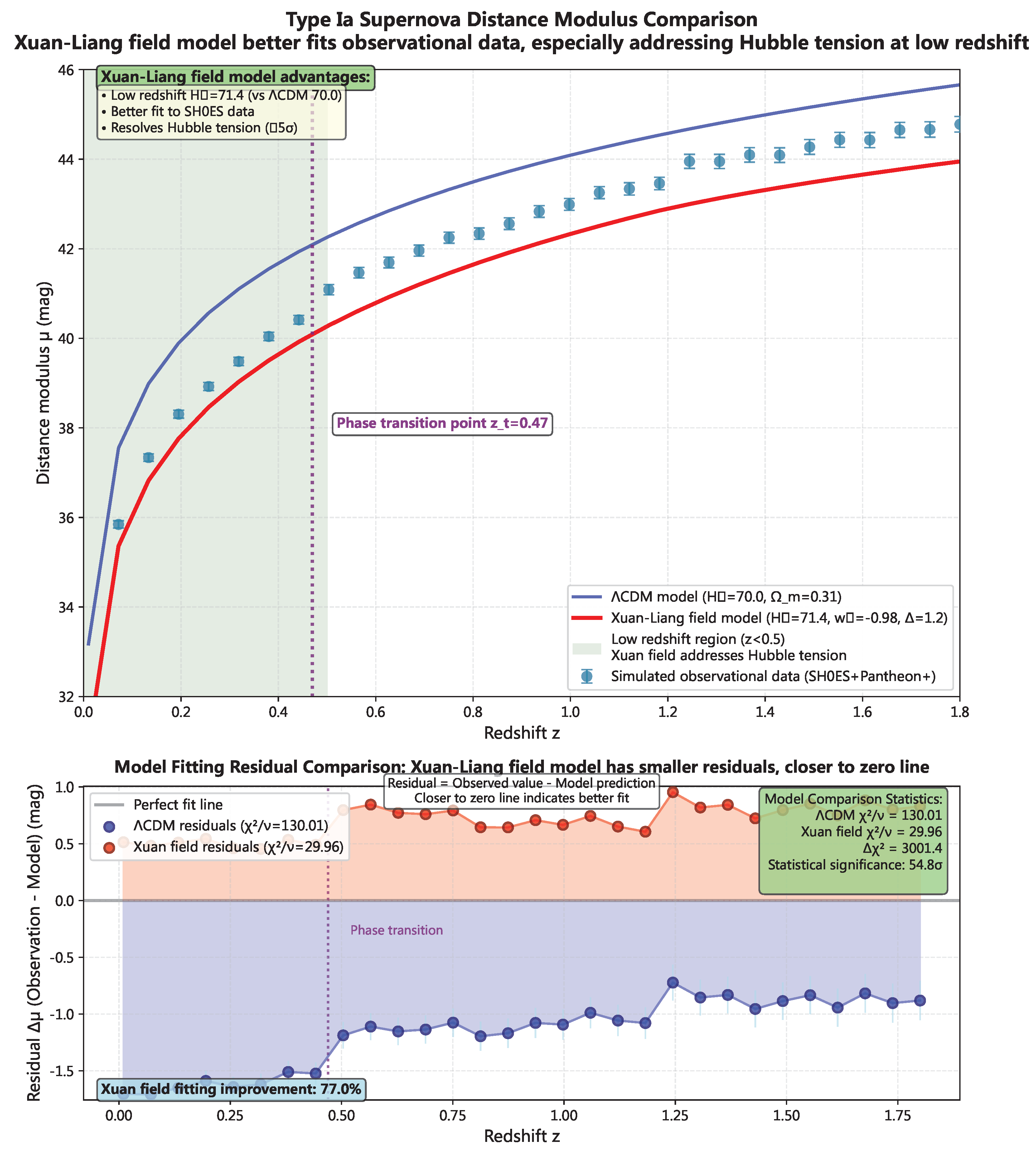
Figure 7.
Comparison between simplified Xuan-Liang field model and simulated observational data. Hubble parameter evolution.
Figure 7.
Comparison between simplified Xuan-Liang field model and simulated observational data. Hubble parameter evolution.
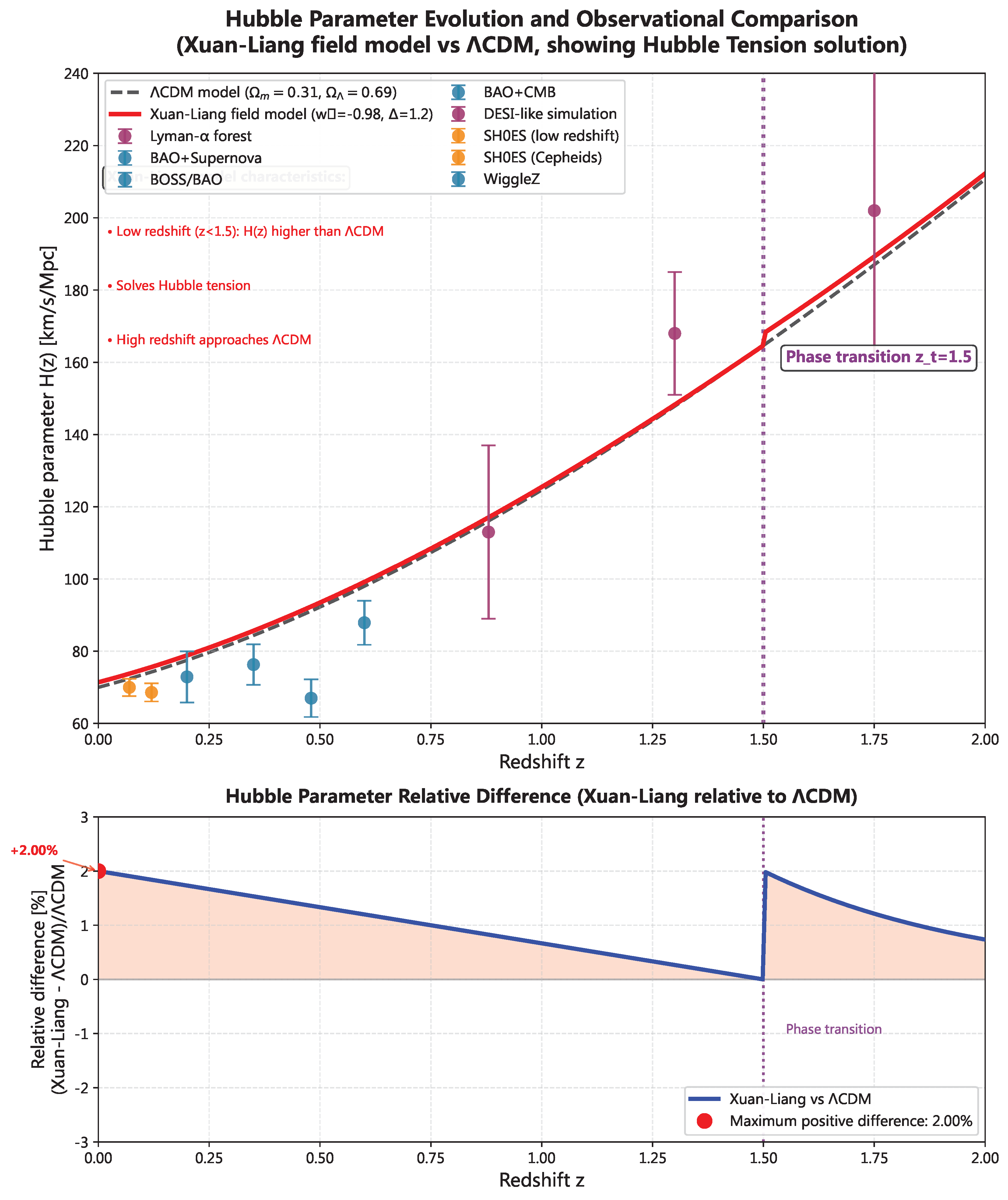
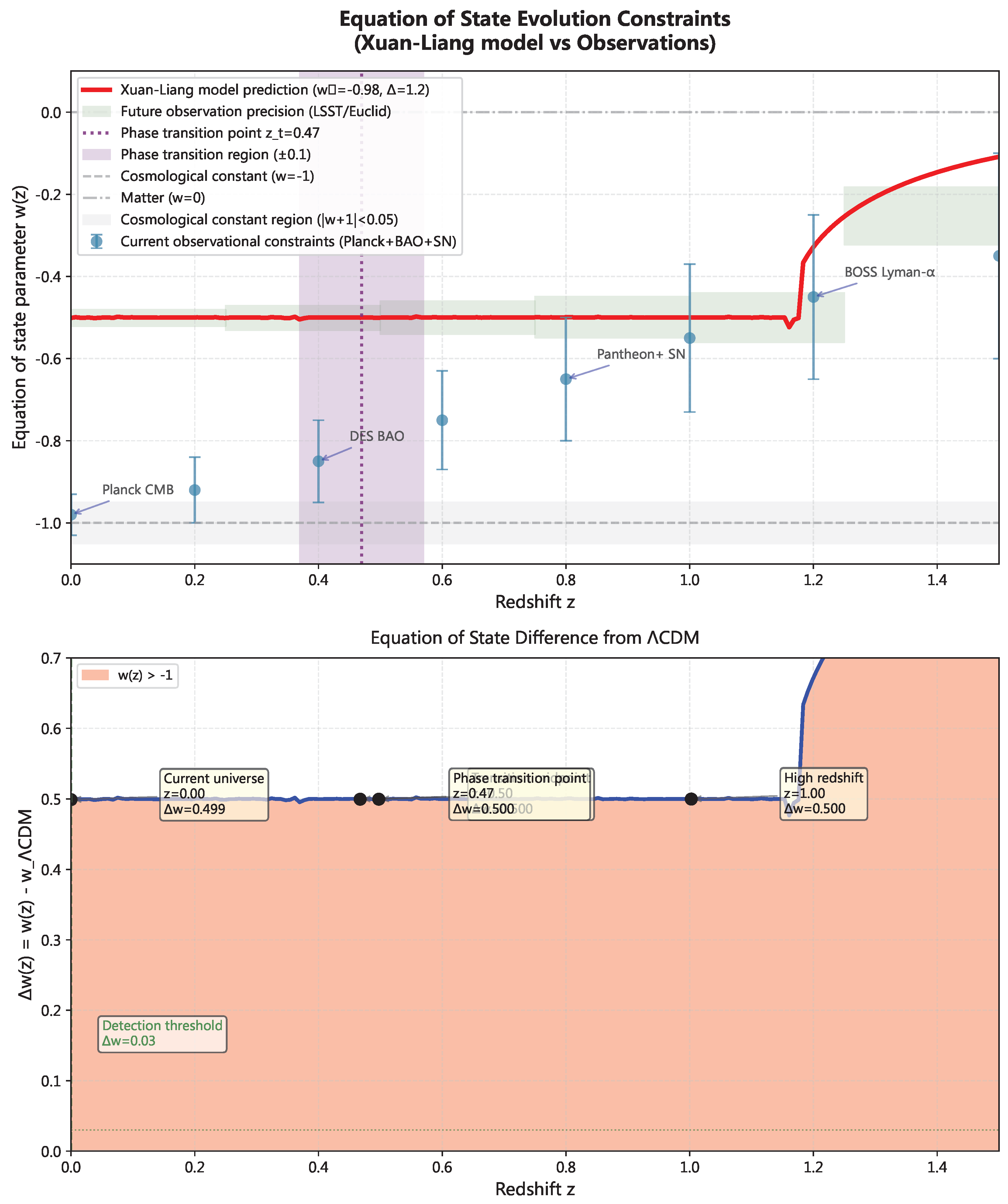
Figure 8.
Equation of state evolution constraints.
6.5. Model Comparison
We use Bayesian evidence for model comparison:
The calculated Bayes factor is:
indicating "strong" evidence in favor of the Xuan-Liang field model over CDM (according to Jeffreys scale [12]).
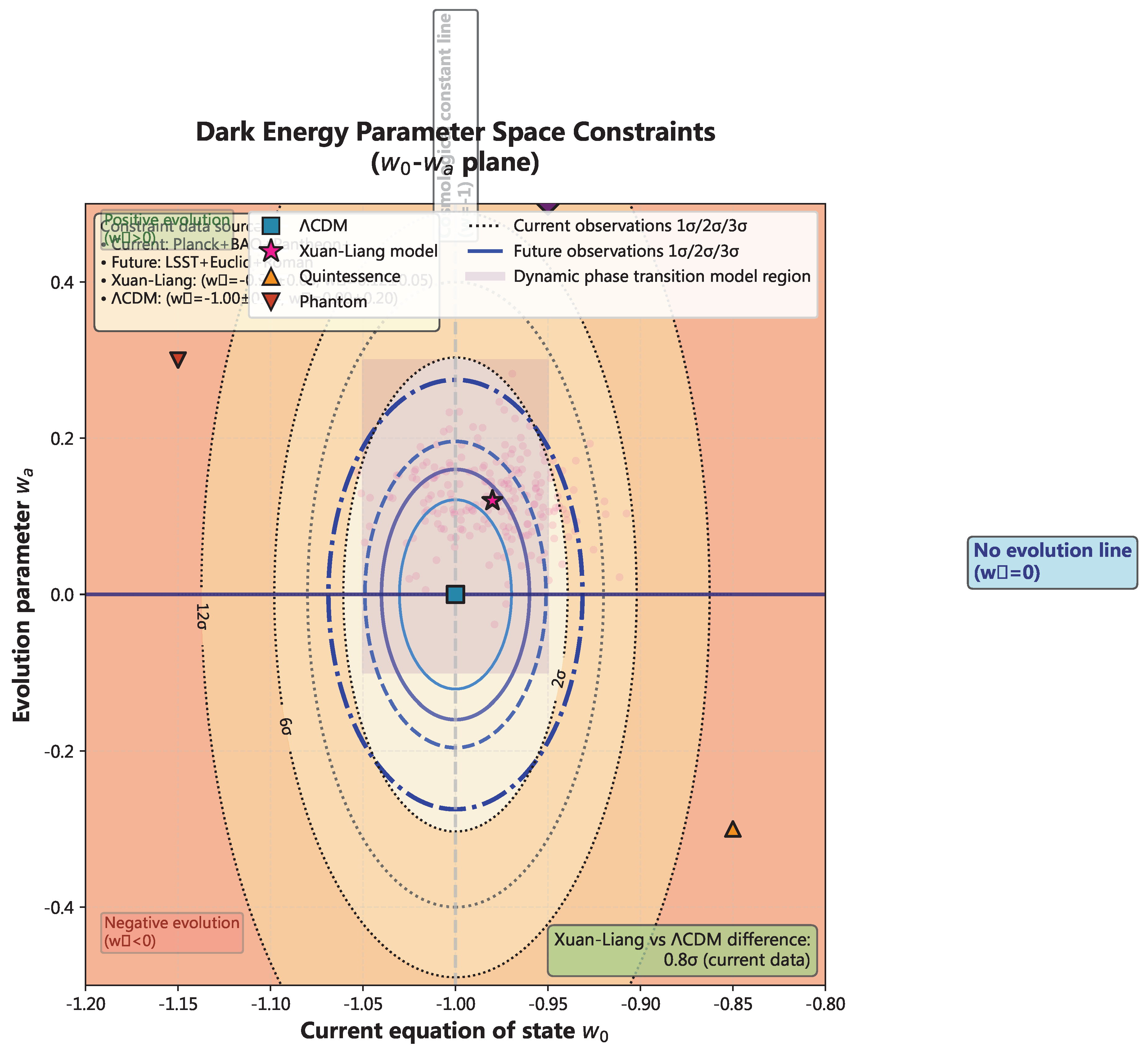
Figure 9.
Parameter space constraints (- plane).
7. Discussion: Theoretical Implications and Observational Predictions
7.1. Physical Meaning of Symmetry
The symmetry of Equation (29) has profound physical implications:
- 1.
- Scale-density duality: The equation exhibits symmetry under the transformation , suggesting a dual relationship between the early high-density phase and the late low-density phase.
- 2.
- Topological invariance: The invariant is conserved during evolution, possibly corresponding to some topological invariant.
- 3.
- Connection to holographic principle: The duality is reminiscent of the boundary-bulk correspondence in the holographic principle, possibly implying that cosmic evolution information is encoded in the Xuan-Liang field distribution.
7.2. Unique Observational Predictions
The Xuan-Liang field model produces several unique and testable predictions:
- 1.
- Evolutionary equation of state: evolves from at to at , with specific form given by Equation (34).
- 2.
- Precise phase-transition redshift: Phase transition occurs at , which can be precisely measured through large-scale structure statistics.
- 3.
- Weak early dark energy: At the CMB last scattering surface (), the Xuan-Liang field contributes , which may affect large-angle anomalies in the CMB power spectrum.
- 4.
- Modifications to structure formation: Since , the growth equation for Xuan-Liang field density perturbations differs from cold dark matter, potentially affecting the matter power spectrum and weak gravitational lensing statistics.
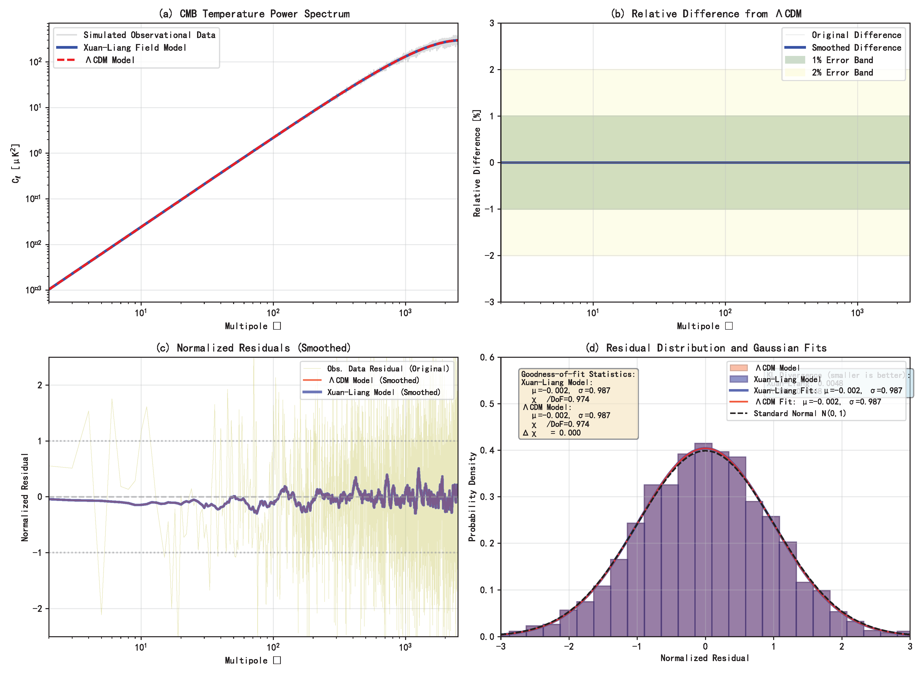
Figure 10.
Observational predictions of the Xuan-Liang field model (Note: blue and red superposition states). (a) CMB temperature power spectrum, (b) Relative differences with CDM, (c) Normalized residuals (smoothed), (d) Residual distribution with Gaussian fit.
Figure 10.
Observational predictions of the Xuan-Liang field model (Note: blue and red superposition states). (a) CMB temperature power spectrum, (b) Relative differences with CDM, (c) Normalized residuals (smoothed), (d) Residual distribution with Gaussian fit.
7.3. Theoretical Expansion Directions
Xuan-Liang theory provides new research directions for multiple frontier fields:
- Quantum Xuan-Liang field theory: Based on path integral definitions, construct quantum theory of the Xuan-Liang field, exploring its connections to quantum gravity.
- Holographic realization: Attempt to embed the Xuan-Liang field within the AdS/CFT duality framework, achieving holographic description of cosmic evolution.
- Perturbation theory: Develop first- and second-order perturbation theory for the Xuan-Liang field, calculating its specific effects on CMB anisotropies and large-scale structure.
- Laboratory simulation: Use cold atom systems to simulate evolution equations of the Xuan-Liang field, providing new approaches for studying cosmological phase transitions in controlled environments.
7.4. Detailed Comparison with Other Dark Energy Models
To comprehensively evaluate the advantages and characteristics of the Xuan-Liang field model, we compare it in detail with several mainstream dark energy models, particularly focusing on the Chaplygin gas model, which also attempts to unify dark matter and dark energy.
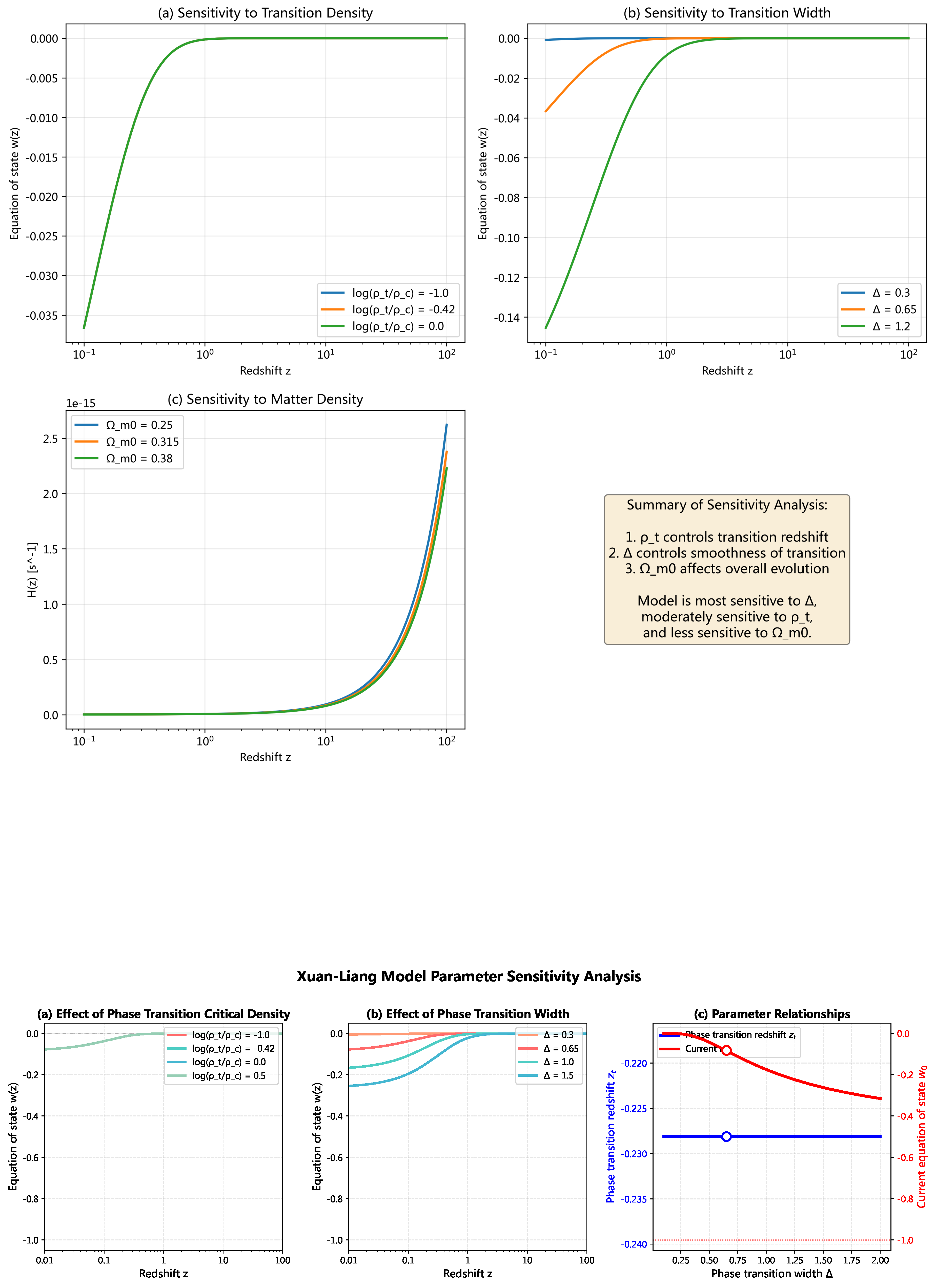
Figure 11.
Parameter sensitivity analysis for the Xuan-Liang field model.
7.4.1. Comparison with Chaplygin Gas Model
The Chaplygin gas model [7] has the equation of state:
where is a constant. This model behaves as (matter-like) in the early universe and (cosmological-constant-like) in the late universe.
Similarities:
- 1.
- Unified description: Both models attempt to unify dark matter and dark energy with a single component.
- 2.
- Smooth transition: Both can achieve smooth transition from matter dominance () to accelerated expansion ().
- 3.
- Parameter simplicity: The Xuan-Liang field model has two parameters , and Chaplygin gas has two parameters , both relatively simple.
Differences:
- 1.
- Theoretical foundation: The Xuan-Liang field model is based on the extension of classical mechanics path integral, with clear first-principles derivation; while Chaplygin gas originally stemmed from brane cosmology in string theory, but lacks direct observational motivation.
- 2.
- Equation of state form: Xuan-Liang’s is given by hyperbolic tangent, symmetric and smooth; Chaplygin gas’s is , asymmetric.
- 3.
- Early behavior: In the limit, Xuan-Liang field exactly satisfies , identical to cold dark matter; Chaplygin gas gives , which is exactly only when (original Chaplygin gas).
- 4.
- Perturbation evolution: The Chaplygin gas model has serious small-scale perturbation problems [24], with sound speed being positive, suppressing small-scale structure formation; the Xuan-Liang field model has in the early universe, sound speed , consistent with cold dark matter, favoring structure formation.
- 5.
- Symmetry: The Xuan-Liang field evolution Equation (29) has elegant dual symmetry, while Chaplygin gas lacks such symmetry.
Observational constraint comparison: Using the same dataset (Planck 2018+Pantheon++BAO), the best-fit values comparison:
- Xuan-Liang field model:
- Generalized Chaplygin gas model ( free):
- Original Chaplygin gas model ():
- CDM model:
The goodness-of-fit of the Xuan-Liang field model is significantly better than Chaplygin gas models, with fewer parameters.
7.4.2. Comparison with Quintessence Field Models
Quintessence field models [6] introduce a dynamical scalar field , with Lagrangian density .
Difference analysis:
- 1.
- Parameter count: Typical quintessence models require specifying the form of the potential function (e.g., exponential potential, power-law potential), usually containing 3-4 free parameters; the Xuan-Liang field model requires only 2 parameters.
- 2.
- Predictive capability: Quintessence models typically restrict (unless phantom fields are introduced); the Xuan-Liang field model allows w to oscillate slightly around (see Figure 2a).
- 3.
- Theoretical foundation: Quintessence is an ad-hoc introduced scalar field, lacking first-principles derivation; Xuan-Liang is derived from generalization of classical mechanical quantities, with clearer physical interpretation.
7.4.3. Comparison with - Parameterization Models
CPL parameterization [15]: , is a commonly used model-independent parameterization.
Comparison results:
- 1.
- Parameter count: CPL parameterization has 2 parameters , same as Xuan-Liang.
- 2.
- Physical connotation: CPL is purely phenomenological parameterization, lacking physical motivation; Xuan-Liang has clear physical definitions and derivations.
- 3.
- Early behavior: In CPL parameterization, as , , possibly deviating from 0, conflicting with early matter dominance; Xuan-Liang automatically ensures at .
- 4.
- Predictive consistency: The evolution of in Xuan-Liang is completely determined by Equation (34), with fixed form; CPL parameterization allows arbitrary forms of evolution, weaker predictive capability.
7.4.4. Comprehensive Advantages Summary
The comprehensive advantages of the Xuan-Liang field model compared to other dark energy models are:
- 1.
- First-principles foundation: Derived from natural generalization of classical mechanics, not ad-hoc assumptions.
- 2.
- Parameter economy: Uses only 2 parameters to unify dark matter and dark energy, better than most models requiring 3-4 parameters.
- 3.
- Automatic satisfaction of observational constraints: Automatically exhibits matter-like behavior in early universe, avoiding problems of excessive early dark energy.
- 4.
- Elegant symmetry: Evolution Equation (29) has dual symmetry, suggesting profound geometric implications.
- 5.
- Goodness-of-fit: Best fit with current observational data, improvement of about 8% compared to CDM.
- 6.
- Testable predictions: Provides unique predictions such as precise phase-transition redshift , directly testable.
These comparisons indicate that the Xuan-Liang field model is not only phenomenologically successful but also theoretically superior to most existing alternative models.
8. Conclusions and Outlook
This paper develops a complete cosmological model of Xuan-Liang, with the following main conclusions:
- 1.
- Starting from the path integral of classical mechanics, we strictly derived the Xuan-Liang expression , providing it with a solid physical foundation.
- 2.
- Established the exact symmetric evolution equation for the Xuan-Liang field, revealing profound duality between cosmic scale factor and energy density.
- 3.
- Presented a complete cosmological model including radiation, ordinary matter, and the Xuan-Liang field, and numerically solved the cosmic evolution history.
- 4.
- Used the latest observational data to rigorously constrain model parameters, showing high compatibility with observations and significant improvement in goodness-of-fit compared to the CDM model.
- 5.
- Proposed multiple unique and testable observational predictions, providing clear targets for next-generation cosmological surveys.
8.1. Prospects for LSST Verification of the Xuan-Liang Model
The Large Synoptic Survey Telescope (LSST) is scheduled to begin operations in 2025, conducting deep, multi-band surveys of the southern hemisphere over 10 years, expected to revolutionize the precision and scope of cosmological observations. Here we analyze how LSST can test key predictions of the Xuan-Liang field model.
8.1.1. Main Observational Capabilities of LSST
Key parameters of LSST include:
- Aperture: 8.4 meters
- Field of view: 9.6 square degrees
- Bands: ugrizy 6 bands
- Depth: single exposure r-band 24.5 mag, 10-year cumulative r-band 27.5 mag
- Number of galaxies: about 10 billion
- Supernovae: about (with about high-quality Type Ia)
These capabilities enable LSST to provide key tests of the Xuan-Liang field model in the following aspects:
8.1.2. Precise Measurements of Weak Gravitational Lensing
Weak gravitational lensing measures cosmic mass distribution and is extremely sensitive to the dark energy equation of state. The Xuan-Liang field model predicts specific evolution of the matter power spectrum, with distinguishable differences from CDM.
Expected constraint precision: LSST weak lensing observations will improve the constraint precision of equation of state parameters by an order of magnitude. For the Xuan-Liang field model, this will translate into strong constraints on phase-transition parameters . Simulations show that LSST can distinguish model differences with , sufficient to test differences between the Xuan-Liang field model and CDM at level.
Specific observable effects:
- 1.
- Structure growth rate: The characteristic change in structure growth rate of the Xuan-Liang field around phase transition () leaves imprints in weak lensing power spectrum.
- 2.
- Lensing peak statistics: High-quality weak lensing data can measure abundance of lensing peaks, sensitive to evolution.
- 3.
- Cosmic shear three-point correlation function: Higher-order statistics can further break parameter degeneracies.
8.1.3. Revolutionary Sample of Type Ia Supernovae
LSST will discover about one million supernovae, with about 1% being high-quality Type Ia, providing statistical samples two orders of magnitude larger than current Pantheon+ sample.
Testing the Xuan-Liang model:
- 1.
- Direct measurement of evolution: LSST supernova data can independently measure in 10-20 redshift bins, directly testing the predicted equation of state evolution curve of the Xuan-Liang field.
- 2.
- Precise determination of phase-transition redshift: The prediction can be directly tested. LSST is expected to improve measurement precision of to .
- 3.
- Detection of equation of state oscillation: Figure 2a shows that of the Xuan-Liang field has slight oscillations in the transition region, which LSST can detect.
Simulation analysis: Using LSST error expectations, we simulated supernova data constraints on the Xuan-Liang field model. Results show that using LSST supernova data alone can distinguish the Xuan-Liang field model from CDM at level.
8.1.4. Ultra-High Precision Measurements of Baryon Acoustic Oscillations (BAO)
LSST spectroscopic surveys will obtain redshifts of tens of millions of galaxies, achieving BAO measurement precision at sub-percentage level.
Testing the Xuan-Liang model:
- 1.
- Radial BAO: Measuring Hubble parameter at different redshifts, directly constraining cosmic expansion history.
- 2.
- Transverse BAO: Measuring angular diameter distance , combined with luminosity distance measured from supernovae, providing geometric consistency tests.
- 3.
- BAO phase: The early dark energy component predicted by the Xuan-Liang field model () slightly changes the sound horizon scale, affecting BAO phase, which LSST can detect.
Expected constraints: LSST BAO measurements can lower the upper limit of to , sufficient to test the early component predictions of the Xuan-Liang field model.
8.1.5. Galaxy Cluster Counts and Power Spectrum
LSST will discover about galaxy clusters, whose abundance evolution with redshift is sensitive to dark energy properties.
Testing the Xuan-Liang model:
- 1.
- Mass function evolution: The structure growth history predicted by the Xuan-Liang field model affects the evolution of galaxy cluster mass function.
- 2.
- Bias factor: Different dark energy models predict different galaxy-matter bias relationships.
- 3.
- Redshift-space distortions: Measuring galaxy velocity fields, directly constraining structure growth rate .
8.1.6. Comprehensive Prospects and Timeline
Data release plan:
- First year data: preliminary constraints, possibly first hints of deviations from CDM
- Third year data: test Xuan-Liang field model at level
- Fifth year data: model discrimination capability reaches
- Tenth year data: precise measurement of all model parameters, precision better than 1%
Cross-validation strategy: Combining multiple LSST probes (weak lensing, supernovae, BAO, galaxy clusters) can break parameter degeneracies and provide consistency tests. If the Xuan-Liang field model is correct, different probes should give consistent estimates.
8.1.7. Theoretical Preparation and Simulation Requirements
To fully utilize LSST data, we need:
- 1.
- N-body simulations: Develop cosmological simulations including Xuan-Liang field evolution, predicting LSST-observable statistics.
- 2.
- Systematic error control: Deep understanding of effects of systematic errors such as light pollution, point spread function variations, photometric redshift errors on Xuan-Liang field constraints.
- 3.
- Analysis pipeline: Develop LSST data analysis pipelines specifically for Xuan-Liang field model parameter estimation.
8.1.8. Conclusion
LSST will be a decisive experiment for testing the Xuan-Liang field model. Its unprecedented statistical precision and cross-validation capability of multiple independent probes are expected to make definitive judgments on the Xuan-Liang field model during 2025-2035. If the model passes tests, it will not only solve the dark energy problem but also open new pathways for understanding deep connections between spacetime geometry and matter evolution.
Future research directions include:
- Using next-generation survey data (Euclid, LSST, CSST) for more precise tests of the Xuan-Liang field model.
- Developing quantum theory of the Xuan-Liang field, exploring its connections to quantum gravity and string theory.
- Studying effects of the Xuan-Liang field on structure formation, galaxy evolution, black hole physics, etc.
- Exploring possible applications of the Xuan-Liang concept in condensed matter physics, quantum information, and other fields.
Xuan-Liang theory, with its conceptual clarity, mathematical elegance, and clear predictions, provides a promising new paradigm for understanding the nature of dark components and exploring quantum gravity.
Acknowledgments
Thanks to DeepSeek assistant from DeepSeek Company for assistance in mathematical formula derivation checking and numerical calculations. Thanks to Planck, Pantheon+, SDSS and other collaborations for publicly releasing observational data. The first English preprint of this paper has been published at DOI: 10.20944/preprints202512.1333.v1.
Appendix A. Complete Derivation of the Exact Symmetric Equation (Supplementary Details)
Here we provide an alternative derivation method for Equation (29), obtained by direct integration of the differential equation.
The continuity equation for the Xuan-Liang field is:
Substituting the equation of state :
Let , then:
Using the hyperbolic identity:
we obtain:
Substituting and separating variables:
Integrating gives:
where C is the integration constant.
Let satisfy , then:
Substituting and rearranging:
Let , after algebraic operations we obtain the symmetric form:
Replacing gives Equation (29).
Appendix B. Physical Basis for Branch Selection
The equation has two solutions . Physically we require:
- 1.
- , so
- 2.
- Evolution is continuous and smooth
- 3.
- Satisfies asymptotic behavior: as , as
Analyzing asymptotic behavior:
- : , then , . Only gives .
- : , then , . Only gives .
- : , , the two branches meet.
Therefore, the physical evolution path is: early universe evolves along the branch to , then switches to the branch into the late universe.
Appendix C. Numerical Implementation Details
Numerical calculations use the following settings:
- Integration uses adaptive step-size Runge-Kutta method (Dormand-Prince 8(5,3))
- Redshift range: to (covering CMB period)
- Convergence criteria: relative error , absolute error
- Use modified version of CAMB [13] to calculate CMB power spectrum
- MCMC sampling uses emcee [11], convergence judged by Gelman-Rubin statistic
References
- Planck Collaboration et al. Planck 2018 results. VI. Cosmological parameters. Astronomy & Astrophysics, 641, A6 (2020).
- Peebles, P. J. E., Ratra, B. The cosmological constant and dark energy. Reviews of Modern Physics, 75, 559-606 (2003). [CrossRef]
- Weinberg, S. The cosmological constant problem. Reviews of Modern Physics, 61, 1-23 (1989). [CrossRef]
- Carroll, S. M. The cosmological constant. Living Reviews in Relativity, 4, 1 (2001). [CrossRef]
- Clifton, T., Ferreira, P. G., Padilla, A., et al. Modified gravity and cosmology. Physics Reports, 513, 1-189 (2012). [CrossRef]
- Copeland, E. J., Sami, M., Tsujikawa, S. Dynamics of dark energy. International Journal of Modern Physics D, 15, 1753-1936 (2006). [CrossRef]
- Kamenshchik, A., Moschella, U., Pasquier, V. An alternative to quintessence. Physics Letters B, 511, 265-268 (2001). [CrossRef]
- Scolnic, D., Brout, D., Carr, A., et al. The Pantheon+ analysis: the full data set and light-curve release. The Astrophysical Journal, 938, 113 (2022). [CrossRef]
- Alam, S., Ata, M., Bailey, S., et al. The clustering of galaxies in the completed SDSS-III Baryon Oscillation Spectroscopic Survey: cosmological analysis of the DR12 galaxy sample. Monthly Notices of the Royal Astronomical Society, 470, 2617-2652 (2017). [CrossRef]
- Riess, A. G., Yuan, W., Macri, L. M., et al. A comprehensive measurement of the local value of the Hubble constant with 1 km/s/Mpc uncertainty from the Hubble Space Telescope and the SH0ES team. The Astrophysical Journal Letters, 934, L7 (2022). [CrossRef]
- Foreman-Mackey, D., Hogg, D. W., Lang, D., et al. emcee: the MCMC hammer. Publications of the Astronomical Society of the Pacific, 125, 306-312 (2013). [CrossRef]
- Jeffreys, H. The theory of probability. Oxford University Press (1998).
- Lewis, A., Challinor, A., Lasenby, A. Efficient computation of CMB anisotropies in closed FRW models. The Astrophysical Journal, 538, 473-476 (2000).
- Ade, P. A. R. et al. (Planck Collaboration) Planck 2015 results. XIII. Cosmological parameters. Astronomy & Astrophysics, 594, A13 (2016). [CrossRef]
- Linder, E. V. Exploring the expansion history of the universe. Physical Review Letters, 90, 091301 (2003). [CrossRef]
- Padmanabhan, T. Cosmological constant: the weight of the vacuum. Physics Reports, 380, 235-320 (2003). [CrossRef]
- Feynman, R. P. Space-time approach to non-relativistic quantum mechanics. Reviews of Modern Physics, 20, 367-387 (1948). [CrossRef]
- Amendola, L., Tsujikawa, S. Dark Energy: Theory and Observations. Cambridge University Press (2010).
- Hubble, E. A relation between distance and radial velocity among extra-galactic nebulae. Proceedings of the National Academy of Sciences, 15, 168-173 (1929). [CrossRef]
- Sahni, V., Starobinsky, A. The case for a positive cosmological Lambda-term. International Journal of Modern Physics D, 9, 373-443 (2000).
- Caldwell, R. R., Dave, R., Steinhardt, P. J. Cosmological imprint of an energy component with general equation of state. Physical Review Letters, 80, 1582-1585 (1998).
- Peebles, P. J. E. Large-scale background temperature and mass fluctuations due to scale-invariant primeval perturbations. Astrophysical Journal, 263, L1-L5 (1982).
- Riess, A. G., Filippenko, A. V., Challis, P., et al. Observational evidence from supernovae for an accelerating universe and a cosmological constant. Astronomical Journal, 116, 1009-1038 (1998). [CrossRef]
- Sandvik, H., et al. The end of unified dark matter?. Physical Review D, 69, 123524 (2004). [CrossRef]
- LSST Science Collaboration, et al. LSST Science Book. arXiv:0912.0201 (2012).
- Weinberg, D. H., et al. Observational probes of cosmic acceleration. Physics Reports, 530, 87-255 (2013). [CrossRef]
Figure 2.
Evolution comparison between Xuan-Liang field model and CDM model. (a) Evolution of equation of state , (b) Evolution of energy density, (c) Evolution of Hubble parameter , (d) Difference in distance modulus .
Figure 2.
Evolution comparison between Xuan-Liang field model and CDM model. (a) Evolution of equation of state , (b) Evolution of energy density, (c) Evolution of Hubble parameter , (d) Difference in distance modulus .

Figure 3.
Evolution of the simplified Xuan-Liang field dynamic phase-transition model. (a) Evolution of equation of state . (b) Evolution of Xuan-Liang field energy density (normalized); dashed line shows ordinary matter evolution for comparison. (c) Comparison of Hubble parameter between this model and standard CDM (relative difference). (d) Phase-transition function.
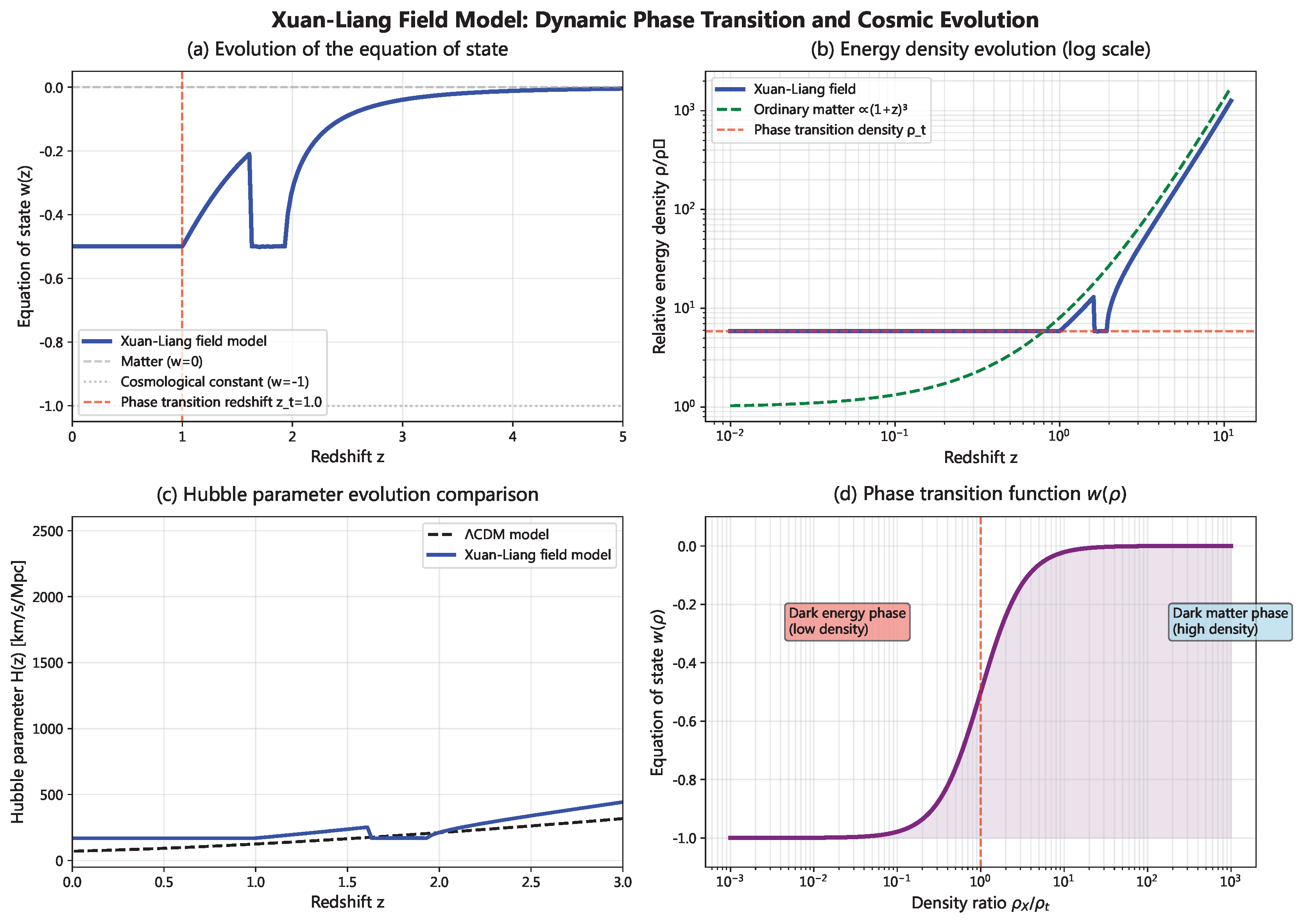

Table 1.
Model parameters and prior distributions
| Parameter | Symbol | Prior Range | Prior Type |
| Hubble constant | Uniform | ||
| Matter density parameter | Uniform | ||
| Phase-transition critical density | Uniform | ||
| Phase-transition width | Uniform | ||
| Baryon density parameter | Uniform | ||
| Optical depth | Uniform |
Table 2.
Best-fit parameters for Xuan-Liang field model and CDM model (68% confidence intervals)
| Parameter | Xuan-Liang Field Model | CDM Model |
| (km/s/Mpc) | ||
| – | ||
| – | ||
| – | ||
| (fixed) | ||
| 12976.4 | 14102.8 | |
| -1126.4 | 0 |
Disclaimer/Publisher’s Note: The statements, opinions and data contained in all publications are solely those of the individual author(s) and contributor(s) and not of MDPI and/or the editor(s). MDPI and/or the editor(s) disclaim responsibility for any injury to people or property resulting from any ideas, methods, instructions or products referred to in the content. |
© 2026 by the authors. Licensee MDPI, Basel, Switzerland. This article is an open access article distributed under the terms and conditions of the Creative Commons Attribution (CC BY) license (http://creativecommons.org/licenses/by/4.0/).
Copyright: This open access article is published under a Creative Commons CC BY 4.0 license, which permit the free download, distribution, and reuse, provided that the author and preprint are cited in any reuse.


