Submitted:
14 December 2025
Posted:
16 December 2025
You are already at the latest version
Abstract
Accurate displacement field measurement by holographic interferometry requires robust analysis of high-density fringe patterns, which is hindered by speckle noise inherent in any interferogram, no matter how perfect. Conventional skeletonization methods, such as edge detection algorithms and active contour models, often fail under these conditions, producing fragmented and unreliable fringe contours. This paper presents a novel skeletonization procedure that overcomes these limitations through a threefold approach: (1) representation of the entire fringe family within a physics-informed, finite-dimensional parametric subspace (e.g., a collection of Fourier-based contours), ensuring global smoothness and connectivity of each fringe; (2) introduction of a robust strip-integration functional, which replaces noisy point sampling with a Gaussian-weighted intensity integral across a narrow strip, yielding a smooth objective function, which is convenient to optimize with standard gradient-based techniques; and (3) a recursive quasi-optimization algorithm that takes into account fringe similarity for efficient and stable identification. The method's efficiency is quantitatively validated on synthetic interferograms with controlled noise, demonstrating significantly lower error compared to baseline techniques. Its practical utility is confirmed by successful processing of a real, interferogram of a bent plate containing over 100 fringes, enabling precise reconstruction of the displacement field that closely matches result of independent theoretical modelling. The proposed procedure provides a reliable tool for processing challenging interferograms where traditional methods may fail to obtain satisfactory result.
Keywords:
holographic interferometry
; fringe skeletonization
; speckle noise
; parametric modeling
; strip integration
; displacement field reconstruction
1. Introduction
Holographic interferometry is a cornerstone optical technique for full-field, non-contact measurement of displacements and deformations in experimental mechanics [1]. Its high sensitivity, enabling resolution of displacements on the order of the light wavelength, makes it invaluable for studying complex deformation phenomena. The accuracy of the method is intrinsically connected with the precision with which the resulting interference fringe patterns can be analyzed [2]. In principle, higher measurement resolution is achieved by analyzing interferograms with a high density of fringes. However, in modern practice, the outcome becomes critically dependent on the chosen digital image processing algorithm, as the manual detection of hundreds of fringes is unreliable [3].
The primary obstacle to automation is the presence of speckle noise – an unavoidable granular interference pattern generated by the random scattering of coherent light from surface micro-roughness, which is intrinsic to any physical hologram [4]. While post-processing filters (e.g., median or Gaussian) can reduce speckle visibility in a digital image, they require a delicate approach. Intensive smoothing can introduce systematic biases that shift the fringe locations, a particularly detrimental effect for high-density patterns where fine details are essential. Consequently, the development of robust, noise-resistant skeletonization algorithms, that can dispense with significant pre-filtering remains an actual problem in optical metrology.
A variety of general-purpose image processing techniques have been applied to fringe identification. For patterns with moderate noise, edge detection algorithms (e.g., Marr –- Hildreth [5], Canny [6] or Shen – Castan [7]) can be employed. However, for high-density patterns corrupted by strong speckle noise, these methods tend to produce fragmented, disconnected edge maps that require complex and often unreliable post-processing to assemble into complete contours.
Active contour models (snakes) and their variants (e.g., Gradient Vector Flow snakes [8,9]) offer a more flexible method by formulating the fringe identification process as a solution to an energy minimization problem [10]. This method has been successfully adapted for fringe analysis [11,12,13,14]; however, it has an inherent limitation when processing highly noisy, dense patterns, which lies in its high sensitivity to the snake’s initial position.
To overcome these limitations, we propose a novel skeletonization procedure that strategically integrates physical prior knowledge with a noise-robust numerical core. Our contribution is threefold:
- Physics-informed parametric modeling. We constrain the search for fringes to a purpose-built, finite-dimensional functional subspace , which is defined by specific parametric curves (e.g., trigonometric polynomials or splines). This subspace is constructed in such a way as to endow its elements with the required properties, such as smoothness, closure, and specific shape, guaranteeing that the identified fringes are physically plausible, connected curves.
- A robust strip-integration functional with local smoothing. For fringe localization we consider the specific functional in the form of a Gaussian-weighted integral of intensity over a narrow strip surrounding the candidate curve. This formulation allows the use of efficient gradient-based optimization techniques. To compute this functional, a continuously differentiable intensity field is first obtained by local bicubic interpolation, described in Subsection 3.1. The resulting functional is smooth with respect to the curve parameters , ensuring stable convergence.
- A recursive quasi-optimization algorithm. Exploiting the geometric similarity of adjacent fringes, the identification process proceeds recursively outward (or inward). The optimal parameters for an identified fringe seed the initial guess for the next, via a simple scaling transformation (quasi-optimization), followed by a full local refinement of all parameters. This strategy dramatically improves computational efficiency and reliability.
The performance of the proposed method is carefully validated. First, using synthetic interferograms with precisely controlled geometry and additive-multiplicative speckle noise, we demonstrate its acceptable accuracy and robustness compared to baseline methods. The error is estimated using two metrics: the Euclidean norm (-norm) of the difference and its maximal absolute value (-norm). Second, we apply the algorithm to a real, challenging interferogram from a bending experiment on a square plate, containing over 100 fringes. The algorithm successfully extracts the complete skeleton, enabling an accurate reconstruction of the displacement field . This result is shown to be in good agreement with an independent analytical solution, obtained in the paper [15], confirming the practical utility and accuracy of the entire procedure.
The remainder of this paper is organized as follows. Section 2 details the proposed skeletonization procedure. Section 3 describes key implementation aspects. Section 4 presents the quantitative validation on synthetic data. Section 5 showcases the application to real high-density interferograms. Finally, Section 6 discusses the results and outlines future work.
2. The Proposed Skeletonization Method
2.1. Physical Origins of Imperfections in Interferograms
To motivate the design choices of the proposed algorithm, it is essential to understand the physical nature of the imperfections present in a raw interferogram. These imperfections, which corrupt the ideal sinusoidal fringe pattern, arise from the optical setup imperfections and the nature of coherent light scattering. They can be categorized by their spatial scale, necessitating different corrective strategies in the digital processing procedure.
In a typical off-axis holographic setup (e.g., the Leith – Upatnieks scheme [2]), the recorded intensity results from the interference of a reference plane wave and an object wave reflected from the specimen surface. In complex notation, these waves are:
where and are the scalar amplitudes, and are the unit polarization vectors of the reference and initial object waves (directly from the laser source), and are the corresponding wave vectors, and is the spatially varying Jones matrix accounting for polarization changes upon reflection from the deformed surface.
The interference of the wavefronts from the specimen’s reference and deformed states yields an intensity pattern of the form [4,16]:
Here, is the phase difference directly proportional to the deformable object out-of-plane displacement , stands for the polarization-induced visibility term and is the contrast variation, induced by coherent noise. A transition between consecutive dark (or bright) fringes corresponds to a displacement increment of .
The terms , and describe large- to medium-scale corruptions:
- Non-uniform background intensity : Caused by uneven illumination, varying surface reflectivity, and polarization effects (). This leads to slow intensity variations across the image.
- Visibility term and contrast variation : The coherence noisy factor (dependent on laser temporal/spectral properties and surface roughness) modulates the overall fringe contrast. The visibility term induced by polarization and speckle decorrelation can further reduce contrast, even to zero.
- Geometric distortion: The non-coaxiality of reference and object beams in off-axis schemes, combined with lens imperfections, introduces a projective distortion between the object plane and the image sensor.
These low-frequency imperfections are corrected in the preprocessing stage (Section 3) via geometric unwarping and local intensity equalization.
The speckle-dependent terms in (1) present the most significant challenge. It is a fine-grained, high-frequency random pattern resulting from two physically unavoidable phenomena: (i) the finite spectral bandwidth of the laser source, and (ii) the random interference of waves scattered by surface micro-roughness. Unlike Gaussian additive noise, speckle is signal-dependent and exhibits characteristic correlation lengths (). Its spatial frequency content often overlaps with that of the high-density fringes themselves, making linear filtering unsuitable as it erodes fringe edges and introduces systematic localization errors.
This multi-scale analysis dictates our algorithmic strategy: large-scale distortions are removed by explicit preprocessing, while the fine-scale speckle noise is addressed not by filtering, but by the main idea of the proposed method – the parametric modeling (Subsection 2.2) and the strip-integration functional (Subsection 2.4) – which provide robustness without distorting the signal.
2.2. Parametric Modeling and Problem Formulation
The goal of skeletonization is to extract a family of planar curves that represent the level sets (fringes) of the phase map from a discretely sampled intensity image I. A fundamental premise of our approach is to treat fringes as continuous geometric entities (curves) rather than collections of disconnected pixels. Consequently, the search for an optimal curve must be performed within a suitable functional space.
Let denote the rectangular image domain. We consider the space of admissible curves to be a set of rectifiable, closed Jordan curves contained in . For any such curve , we define a functional as the normalized integral of the image intensity over its support:
where is an appropriate measure on . In the simplest case, where the support is the one-dimensional curve itself, is the arc-length measure (), and the normalization factor is the total curve length . This yields the line-integral functional:
The choice of measure and its domain will be generalized in Subsection 2.4 to define more robust functionals. The core optimization problem is to find curves within a constrained set that extremize this functional. For an ideal, normalized interferogram where the low-frequency imperfections from (1) are absent (, ) and speckle noise is removed, the intensity is proportional to . The bright fringes (intensity maxima) correspond to curves that maximize , while dark fringes (minima) correspond to its minimizers. In a real, noisy image, the functional must be extremized despite the corruptions described in Subsection 2.1.
However, operating directly in the infinite-dimensional space is intractable and ignores the crucial physical prior: the expected fringe family possesses a specific global structure. Instead of regularizing the problem within (as active contours do), we constrain the solution a priori to a finite-dimensional subspace . This subspace is defined by a parametric model:
where is a vector of parameters, and the mapping is continuously differentiable. The choice of the model takes into account our a priori knowledge about the deformation. For instance, for the bending of a centrally loaded, clamped plate, the fringes are expected to be nested, closed, and quasi-concentric curves, which can be effectively modeled by a family of perturbed circles or ellipses (see Subsection 3.4).
By restricting the search to , the infinite-dimensional variational problem of extremizing over reduces to a finite-dimensional optimization problem over the parameter space :
This is the core conceptual shift from other methods: the smoothness, connectivity, and global shape of the solution are built into the search space , rather than being enforced via penalty terms during optimization.
2.3. Discretization and Coordinate System
The image data I is provided as a discrete matrix of size , where r and c are integer row and column indices. To connect the continuous formulation with the discrete data, we establish a fixed coordinate system. We assume a unit pixel pitch and place the origin of the Cartesian coordinates at the center of a chosen reference pixel with indices . The correspondence between a pixel and the coordinates of its center is then given by:
This mapping is illustrated in Figure 1.
2.4. Variants of the Functional
The core of the skeletonization method is the optimization of a functional that measures how well a candidate curve aligns with a fringe. We trace its development from a naive discrete form to the final robust, continuous formulation.
2.4.1. Point-Sampling Along the Curve
The most direct approach is to rasterize the curve and sum the intensities of its pixels:
where is the set of pixels that rasterize the curve, and is their number (an integer measure of curve length). This functional is discontinuous with respect to , it means that a small parameter change can alter the set , causing a jump in the sum. This discontinuity precludes the use of gradient-based optimization.
2.4.2. Line-Integration with Interpolation
To obtain a smooth functional, we first construct a -continuous intensity field via bicubic interpolation (detailed in Subsection 3.1). Replacing the discrete sum with a normalized line integral yields:
where is the curve length. is now continuously differentiable, enabling gradient-based optimization. However, it remains sensitive to speckle noise, as it samples intensity only along an infinitesimally thin path.
2.4.3. Point-Sampling Over a Strip
To improve robustness, we consider a strip of width around the curve. A discrete, robust functional can be defined by summing pixel intensities within this strip, weighted by their approximate Gaussian distance to the curve:
where is the set of pixels whose centers lie within the strip , is the minimal distance from the pixel center to the curve, and . This choice of weight function is motivated by the statistical nature of speckle noise nature. The functional averages over many pixels, reducing the impact of speckles. However, it shares the discontinuity flaw of due to the discrete pixel set .
2.4.4. Strip-Integration with Interpolation
The final, optimal form combines the robustness of strip averaging with the smoothness of continuous integration. We define the strip-integration functional as the normalized, weighted area integral over the continuous strip:
where, is the minimal Euclidean distance between and the curve. The functional, , is both robust to noise (due to area averaging) and continuously differentiable in (due to the smoothness of , G, and the parametric curve). It is the functional used in our final algorithm.
3. Numerical Implementation
The evaluation of and requires efficient numerical techniques for interpolation and integration.
3.1. Bicubic Interpolation Scheme
To obtain the intensity field from the pixel matrix , we employ a compact bicubic formula. For a point in a grid cell with corners at pixel centers, the interpolation is:
where , are local coordinates within a cell of the interpolation grid. The integer-valued indices and , which locate the pixel, are functions of the coordinates:
The constant matrix and the matrix (now with understood as the outputs of (6)) are:
The sixteen elements of are finite-difference approximations of the intensity and its derivatives at the four cell corners, computed from the neighborhood of the pixel :
for . This scheme guarantees that is a function across cell boundaries, providing the smoothness required for stable gradient computation. The example of interpolation is shown in Figure 2.
3.2. Numerical Quadrature
The line integral (4) is approximated by discretizing the curve into n segments. For a parametric curve , , we use the trapezoidal rule:
where . The discretization step is chosen adaptively based on the curve’s local curvature to ensure at least one sample per intersected pixel:
In case of strip integration the denominator of (5) can be computed more convenient analytically:
using the expansion for the Jacobian determinant, J, of the coordinate transformation from (curve parameter and normal offset) to :
Substituting this relation into (5) brings it to a form similar to (4):
This integral is approximated by summing contributions from triangular prisms formed by adjacent sample points:
where are the coordinates of a point along the normal at , and is the volume of a triangular prism with base :
The first multiplier here is a height of the approximating prism, while the second one is triangle area, computed through coordinates of its corners:
3.3. Discrete Differential Operators for Accurate Rasterization
The transition from continuous parametric curves to the discrete pixel grid is a critical step that, if done naively, can introduce systematic errors comparable to the inter-fringe spacing in high-density patterns. To achieve sub-pixel accuracy and topological correctness (4-connectivity), we introduce a unified approach based on integer-valued discrete differential operators. These operators analyze the local geometry of the curve directly in pixel-index space, enabling efficient and exact rasterization of both the curve and the surrounding strip.
3.3.1. First-Order Operator: Tangent Direction and Curve Rasterization
Given two consecutive pixel centers and along a discretized curve, we define the first-order discrete directional operator:
This compact formula serves three purposes simultaneously:
- Direction defining: It maps the 9 possible neighbor vectors to unique integers in the range . This mapping is shown in Figure 3.
- Neighborhood Filter: The sum of the cubic terms, acts as a filter because for , the identity holds, while if a parameter step is too large and causes a jump to a non-adjacent pixel, the sum makes (within 2 pixels from ), flagging an invalid "skip".
- Adaptive Step Control: This flag triggers an adaptive adjustment of the parametric step : if a skip is detected; if (meaning the parameter advanced but the pixel did not change). Crucially, we use asymmetric coefficients (, ) to prevent resonant cycling near stationary points, ensuring robust convergence.
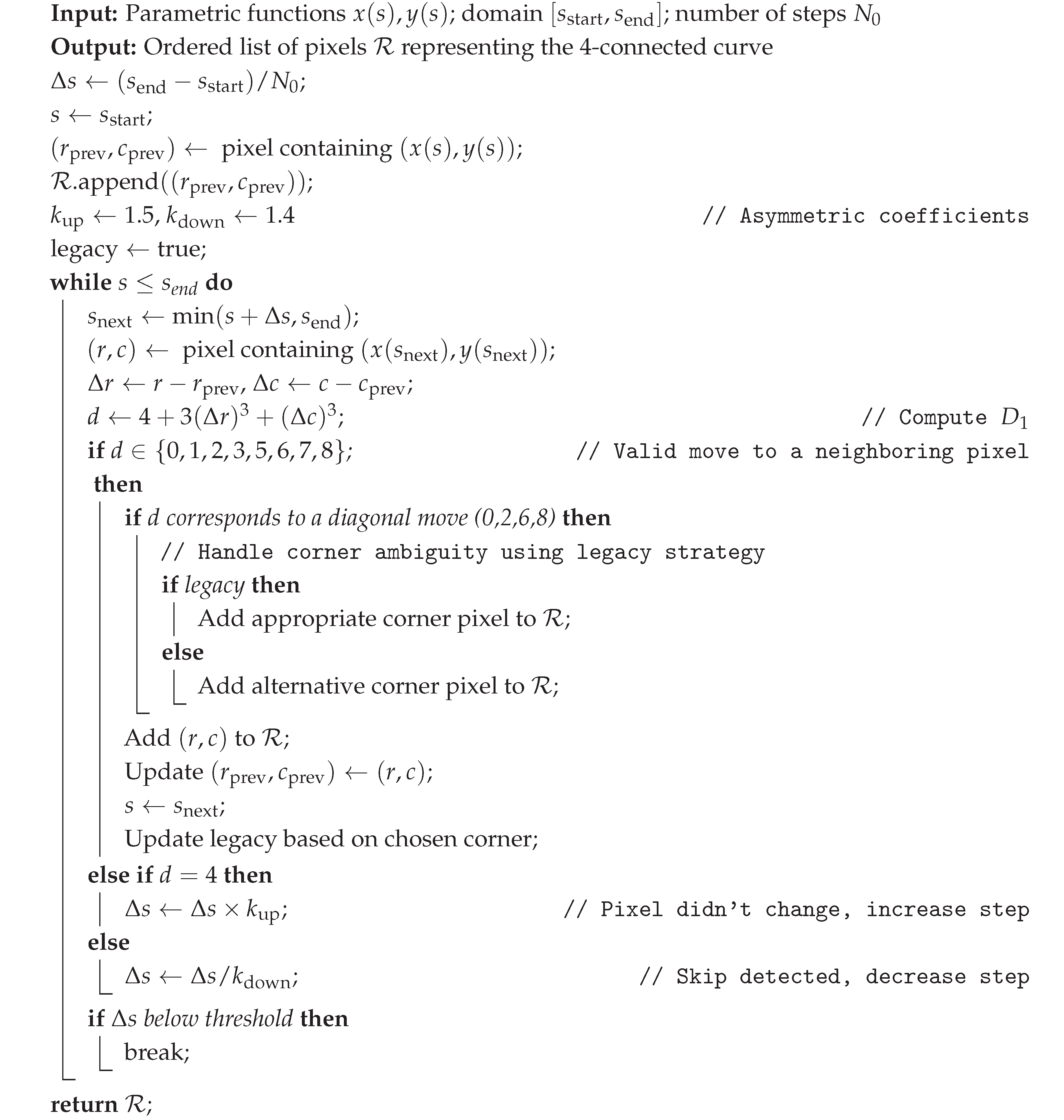
The operator is the core of the curve rasterization algorithm. Its scheme is shown in the Appendix A (Algorithm 1). The algorithm marches along the continuous curve , adaptively adjusting to produce an ordered, 4-connected list of pixels . A key subtlety is the handling of diagonal moves: when the curve passes through a pixel corner, there are two equally valid 4-connected paths. In such cases, the algorithm use a special variable, which memorizes the choice made at the previous step, ensuring a smooth, consistent rasterization without jagged artifacts.
3.3.2. Second-Order Operator: Local Curvature and Strip Rasterization
Rasterizing a strip of width around a curve requires understanding the local curvature to avoid gaps or overlaps in the coverage. Given three consecutive pixel centers of the already rasterized curve, we define a second-order operator that classifies the local shape. Let and . We define the signs of their components as integers: and . The configuration is then defined as:
After shifting and clamping to the valid range of physically realizable 4-connected triples, we obtain the final formula used in the implementation:
The operator evaluates to one of 16 integer values, each corresponding to a distinct local configuration of the three points (see Figure 4). Geometrically, it approximates the discrete curvature. For example:
- indicates nearly linear motion (up, left, right, down), warranting a simple rectangular strip fill.
- indicates a smooth turn, requiring a circular sector fill to cover the curved corner of the strip without gaps.
- corresponds to inflection or "return" points, necessitating a combined fill (e.g., a half-circle plus strips).
Based on the value of , the strip rasterization algorithm (Algorithm (2) in Appendix A) selects an optimal geometric primitive (line strip or circular arc) and fills the corresponding pixels within distance from the central pixel . A distance mask ensures that if a pixel is covered by multiple primitives, the smallest distance to the central curve is retained, and the corresponding Gaussian weight is assigned. This approach guarantees a skip-free, accurate, and weight-aware rasterization of the continuous strip .
3.4. Parametric Models for Fringe Contours
The choice of the parametric subspace is dictated by the expected physics of the deformation. For a broad class of problems involving axisymmetric or nearly axisymmetric bending of plates and membranes, the fringe contours are expected to be closed, nested, quasi-concentric curves. We introduce two related parametric families that efficiently described such shapes while offering sufficient flexibility to capture deviations from ideal geometry.
3.4.1. Perturbed Circle Model
The most natural model for quasi-circular fringes is a perturbed circle, where the constant radius of a circle is replaced by a periodic function of the polar angle . In Cartesian coordinates with an origin at , this is expressed as:
where the radius function is given by a trigonometric polynomial:
Here, is a base radius, is the center, and are the perturbation coefficients. Setting all recovers a perfect circle of radius r centered at . The shift in harmonic indices (using instead of ) ensures that the lowest-order perturbation already affects the shape, leaving the coefficients and implicitly absorbed into r and the center coordinates.
An equivalent, sometimes computationally convenient, representation expands (8) directly into a Fourier series:
where the coefficients are linear combinations of . It is simple to show that , , and the first harmonics are primarily governed by the “coarse” parameters , while higher harmonics depend on the perturbation coefficients. This structure naturally suggests a two-stage optimization strategy:
- Quasi-optimization: Vary only the coarse parameters to quickly locate the approximate position and scale of the fringe.
- Full optimization: Refine all parameters to capture fine shape details.
The total number of parameters is . In our experiments with plate bending, (giving 33 parameters) proved sufficient to accurately represent fringes even under significant nonlinear deformation.
3.4.2. Perturbed Ellipse Model
For specimens with pronounced anisotropy or non-axisymmetric boundary conditions, the fringe contours may exhibit a preferred elliptical orientation. The model can be generalized to a perturbed ellipse by introducing semi-axes a and b () and an orientation angle :
where
When , this relation reduces to , and the model reverts to the perturbed circle (8). The perturbation is now applied relative to the elliptical base shape and is oriented with it (via the phase shift ). The coarse parameter set for this model is , totaling parameters.
3.4.3. Parameter Constraints and Initialization
To ensure physical plausibility and improve optimization convergence, constraints are applied: ; perturbation coefficients are bounded ( to prevent self-intersection); and for the ellipse, . The initial guess for the first (innermost) fringe is obtained via a coarse search: the image center is estimated from intensity function cross-sections (), then r (and later) is varied until a local extremum of is found. For subsequent fringes, the parameters of the previous fringe are scaled outward by a factor slightly greater than one to provide a good starting point for the quasi-optimization step.
These parametric models, combined with the strip-integration functional and the rasterization operators, constitute the proposed skeletonization framework. However, before proceeding to the experimental validation of its performance in Section 4, it is necessary to prepare the intensity matrix to reduce the influence of speckle noise.
3.5. Local Intensity Equalization Algorithm
Raw interferograms often exhibit slow spatial variations in background intensity and contrast due to uneven illumination and polarization effects (see Subsection 2.1). To normalize these variations without distorting the fringe positions, we employ a local intensity equalization procedure based on quantile statistics within sliding windows.
3.5.1. Local Quantile Computation
Before processing the intensity matrix it is necessary to remove areas of the image without fringes, that contain no fringes, retaining only the useful region. Furthermore geometric distortion correction must be applied to compensate for the misalignment between the camera lens axis and the object beam. The example of this procedure, which we will call the geometric correction, is shown in Figure 5.
Let denote the geometrically corrected intensity matrix of size . For each pixel considered as a potential window center, we define a local block of size :
where and are reflection-padding functions that handle boundary pixels:
This padding ensures that windows near image boundaries remain fully populated without introducing artificial discontinuities.
For each block , we compute two statistics: the lower quantile and the upper quantile at probability levels and , respectively (typically ). These quantiles estimate the local minimum and maximum intensity while being resistant to outlier pixels caused by speckle noise:
3.5.2. Interpolation and Normalization
The quantiles and are computed only on a coarse grid with spacing to reduce computational cost. To obtain values at every pixel , we use linear interpolation:
The normalized intensity at each pixel is then obtained by linear rescaling:
This operation maps the local intensity range approximately to , effectively compensating for low-frequency inhomogeneities while preserving the high-frequency fringe structure.
3.5.3. Parameter Selection
The window size q is chosen to be several times larger than the expected inter-fringe distance but smaller than characteristic scales of illumination non-uniformity. In our experiments with square plates, pixels (covering about 3–4 fringes) worked well. The quantile level provides a good compromise between rejecting speckle outliers and retaining true fringe extrema. The equalization is applied once after geometric correction and, if needed, repeated after optional Fourier filtering to compensate for global intensity shifts introduced by the filter.
3.6. Complete Skeletonization Algorithm
Integrating all components described in the previous subsections, we present the complete procedure for automated fringe skeletonization. The algorithm proceeds recursively from the innermost to the outermost fringe, taking into account the quasi-similarity property. The main steps are illustrated in Figure 6. The algorithm iteratively identifies fringes until one of the three termination conditions is met:
- The last computed intensity integral is equal to zero;
- The last identified fringe lies outside the image boundaries;
- The required (or preset) number of fringes has been identified;
3.7. Synthetic Interferogram Generation
To quantitatively validate the proposed algorithm under controlled conditions, we developed a virtual interferogram generator that produces images with known pattern geometry and physically realistic noise characteristics. The generator taking into account two key aspects: (1) the typical fringe pattern of a bent square plate, and (2) the corruption mechanisms described in Subsection 2.1.
3.7.1. Ideal Fringe Geometry via Morphing
The underlying displacement field is modeled by a family of closed curves that morph smoothly from a circle at the center to a square at the boundary, parameterized by a morphing parameter . In the first octant (), the curve consists of a straight segment and a curved segment that ensures continuity:
The full curve over all angles is obtained by symmetric replication. Equivalently, it can be expressed compactly as:
where
The ideal, noise-free intensity pattern is then defined as a periodic function of :
where k controls the fringe density. The mapping is obtained by numerically solving the transcendental equation:
for at each grid point.
3.7.2. Physically Motivated Noise Model
The ideal intensity is corrupted by two noise sources derived from the physical model in Subsection 2.1, which presents the general formula for corrupted intensity (1); however the terms describes speckle noisy, were not specified. Accurately defining of these terms is a complicated problem, which was considered in a huge amount of works (e. g. [16,17,18]). For this paper, it is enough to mark that speckle noise consists of three parts, which related with reflected surface factor, depended on its roughness, spatial and temporal coherence:
where c is the speed of light in vacuum, is the laser spectral linewidth, the path length difference, D is the diameter of the illuminated object area and is the characteristic speckle size:
Here, is the laser wavelength, z is the distance from object to observation plane and is the reflected surface roughness parameter. The resulting speckle noise can be modeled as the product of different coherence terms and the surface factor, which is obtained empirically.
In practice, for rapid commutation and parameter studies, it is convenient to employ a simplified combined noise model, constructed as stochastic perturbations of phase difference and amplitude:
where k controls the overall noise level and , are independent stochastic processes with correlation:
where is the Bessel function. This model approximates the statistical properties of speckle while remaining computationally efficient.
3.7.3. Error Metrics
For each synthetic image, the exact curves are known analytically. This allows us to define rigorous error metrics for any skeletonization result :
These metrics are used in Section 4 to quantitatively compare the performance of different methods.
3.8. Implementation Details.
The described skeletonization procedure has been implemented in a custom C++ program. This program is capable of performing all steps of the proposed algorithm (see Figure 6):
- Geometric correction;
- Filtering in the frequency domain with different kernels;
- Intensity equalization, as described in Subsection 3.5;
- Localization of the image center;
-
Recursive identification of fringes, which includes:
- (a)
- Initializing of parametric curve (Subsection 3.4.1 and Section 3.4.2);
- (b)
- Computing of the intensity integral (Subsection 2.4) using numerical quadratures (Subsection 3.2);
- (c)
-
Defining of the approximation curve’s parameters by one of the optimization methods:
- Advanced Coordinate Descent with Nesterov’s Acceleration for fastest convergence (typically 20-30 iterations per fringe) (e. g. [19]).
- Nelder – Mead simplex method when derivative information is not readily available (robust but slightly slower).
- Conjugate Gradient method for highest precision in final refinement (used only when the highest accuracy is required, despite longer computation time).
An example of the preprocessing of a real interferogram, performed using the developed program, is shown in Figure 7.
Apart from that, the program contains a set of standard tools for working with images and includes a custom generator of synthetic fringe patterns, a described in Subsection 3.7. The generator accepts the following control parameters:
- Fringe density k (number of fringes across the field);
- Speckle noise, dependent on surface roughness parameter and the laser spectral linewidth;
- Noise models the influence of non-uniform illumination;
For each generated image, the exact curves are known analytically. This allows for the quantification of the algorithm errors.
The main computational cost of the algorithms associated with the strip-integrating procedure. Each evaluation of requires operations, where M is the number of quadrature points in the strip discretization. With N fringes and an average of K optimization iterations per fringe, the total cost is . In practice, for a image with 100 fringes, the algorithm completes in 2 – 3 minutes on a standard desktop CPU, making it suitable for practical laboratory use.
4. Validation on Synthetic Interferograms
We compared the efficiency of fringe identification with different variants of the intensity integral, using the metrics defined in Subsection 3.7.3. Figure 8 demonstrates that slightly noisy images, both methods have similar performance, whereas for highly noisy patterns the stripe-integration method has a significant advantage over the line-integration. Moreover, as it is shown in Figure 9, the stripe-integration method is capable of identifying fringes in images with noise levels as high as 95%, where it is hardly possible to differ the fringes even visually.
5. Application to Real High-Density Interferograms
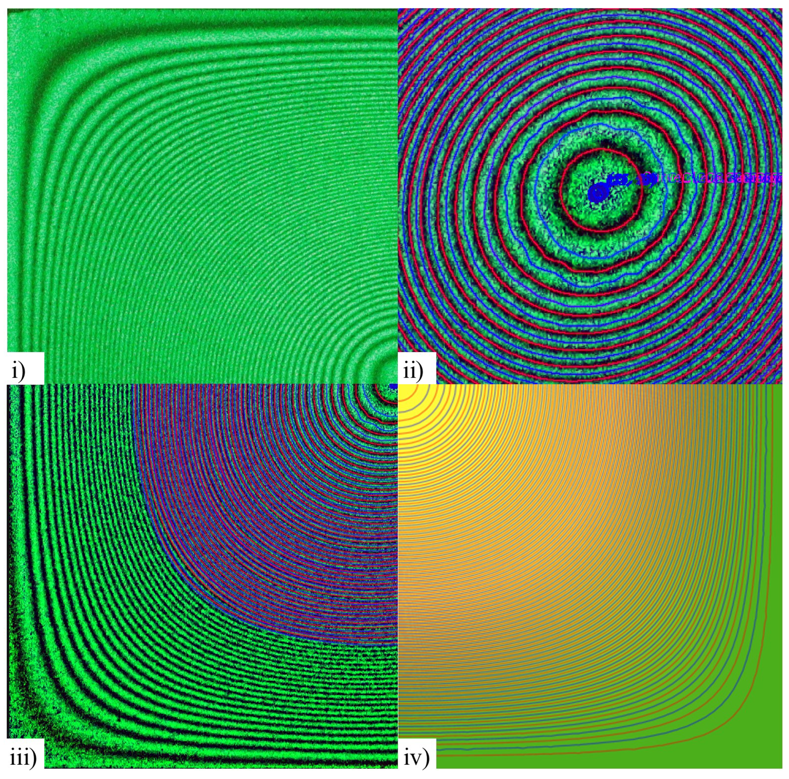
To validate the proposed algorithms, it was tested on a real hologram, obtained from a bending experiment on a square plate. The plate (copper, side length 6 cm, thickness 184 m) was subjected to a uniform transverse load in a holographic interferometry setup (Leith – Upatnieks off-axis scheme with a solid-state laser, nm). Interferograms were recorded for several load increments. The most challenging case, with a deflection generating over 100 fringes (shown in Figure 10i)), was selected for analysis.
The set of identified fringes (red and blue lines in Figure 10ii) and Figure 10iii)) was compared with the results (Figure 10iv)), obtained from theoretical modeling, presented in [15]. As shown in Figure 10, the identified fringes are in good agreement with isolines of deformed surface, demonstrating the acceptable accuracy of the proposed procedure.
6. Conclusion
This paper presents a novel, robust method for skeletonizing fringe patterns in holographic interferometry. By constraining the solution to a physics-informed parametric subspace and employing a strip-integration functional, the method achieves high accuracy and stability in the presence of strong speckle noise, where conventional techniques may fail. Quantitative validation on synthetic data demonstrated a significant reduction in error compared to baseline methods. The practical utility was confirmed by successfully processing a real interferogram with over 100 fringes, the results of which closely matched those of an independent theoretical model.
The main limitation of the algorithm is the need to select an appropriate parametric model beforehand. Thus, the method is most effective when the fringe family topology is known to be a set of nested, simply connected curves. It may be less effective for patterns featuring fringe bifurcations, interruptions, or multiple disconnected families without significant modifications. In the future, the concept of quasi-similarity and recursive search may be modified to a more powerful paradigm for handling complex topologies.
Author Contributions
Conceptualization, methodology, software, validation, writing – original draft preparation, S.L.; resources, investigation, A.D.; writing – review and editing, S.L. and A.D. All authors have read and agreed to the published version of the manuscript.
Funding
This research was supported by the Russian Science Foundation (grant No 23-19-00866).
Institutional Review Board Statement
Not applicable.
Informed Consent Statement
Not applicable.
Data Availability Statement
Data are contained within the article.
Conflicts of Interest
The authors declare no conflicts of interest.
Appendix A: Rasterization Algorithms Pseudocode
| Algorithm 1:Adaptive Curve Rasterization using First-Order Operator |
 |
| Algorithm 2:Strip Rasterization using Second-Order Operator |
|
References
- Kobayashi, A. Handbook on experimental mechanics; Prentice-Hall, 1987.
- Vest, C. Holographic Interferometry; Wiley, 1979.
- Malacara, D.; Servin, M.; Malacara, Z. Interferogram analysis for optical testing; Taylor & Francis, 2005.
- Kreis, T. Handbook of holographic interferometry: optical and digital methods; John Wiley & Sons, 2006.
- Marr, D.; Hildreth, E. Theory of edge detection. Proceedings of the Royal Society of London. Series B. Biological Sciences 1980, 207, 187–217.
- Canny, J. A computational approach to edge detection. IEEE Transactions on pattern analysis and machine intelligence 2009, pp. 679–698.
- Shen, J.; Castan, S. An optimal linear operator for step edge detection. CVGIP: Graphical models and image processing 1992, 54, 112–133. [CrossRef]
- Xu, C.; Prince, J.L. Gradient vector flow: A new external force for snakes. In Proceedings of the Proceedings of IEEE computer society conference on computer vision and pattern recognition. IEEE, 1997, pp. 66–71.
- Xu, C.; Prince, J.L. Snakes, shapes, and gradient vector flow. IEEE Transactions on image processing 1998, 7, 359–369. [CrossRef]
- Kass, M.; Witkin, A.; Terzopoulos, D. Snakes: Active contour models. International journal of computer vision 1988, 1, 321–331. [CrossRef]
- Li, B.; Acton, S.T. Active contour external force using vector field convolution for image segmentation. IEEE transactions on image processing 2007, 16, 2096–2106. [CrossRef]
- Tang, C.; Lu, W.; Cai, Y.; Han, L.; Wang, G. Nearly preprocessing-free method for skeletonization of gray-scale electronic speckle pattern interferometry fringe patterns via partial differential equations. Optics letters 2008, 33, 183–185. [CrossRef]
- Tang, C.; Ren, H.; Wang, L.; Wang, Z.; Han, L.; Gao, T. Oriented couple gradient vector fields for skeletonization of gray-scale optical fringe patterns with high density. Applied optics 2010, 49, 2979–2984. [CrossRef]
- Li, Y.H.; Chen, X.J.; Qu, S.L.; Luo, Z.Y. Algorithm for skeletonization of gray-scale optical fringe patterns with high density. Optical Engineering 2011, 50, 087003–087003. [CrossRef]
- Lychev, S.; Digilov, A.; Djuzhev, N. Galerkin-Type Solution of the Föppl–von Kármán Equations for Square Plates. Symmetry 2024, 17, 32.
- Eichhorn, N.; Osten, W. An algorithm for the fast derivation of line structures from interferograms. Journal of Modern Optics 1988, 35, 1717–1725. [CrossRef]
- Goodman, J.W. Speckle phenomena in optics: theory and applications; Roberts and Company Publishers, 2007.
- Dainty, J.C. Laser speckle and related phenomena; Vol. 9, Springer science & business Media, 2013.
- Wang, Q.; Li, W.; Bao, W.; Zhang, F. Accelerated randomized coordinate descent for solving linear systems. Mathematics 2022, 10, 4379. [CrossRef]
Figure 1.
Relationship between pixel matrix indices and the continuous Cartesian coordinate system . The grid represents the pixel centers. The origin is fixed at the center of the reference pixel with indices . The coordinates of point E (the center of pixel ) are , following Equation (3). The vertices denote the corners of a pixel, located at offsets from its center.
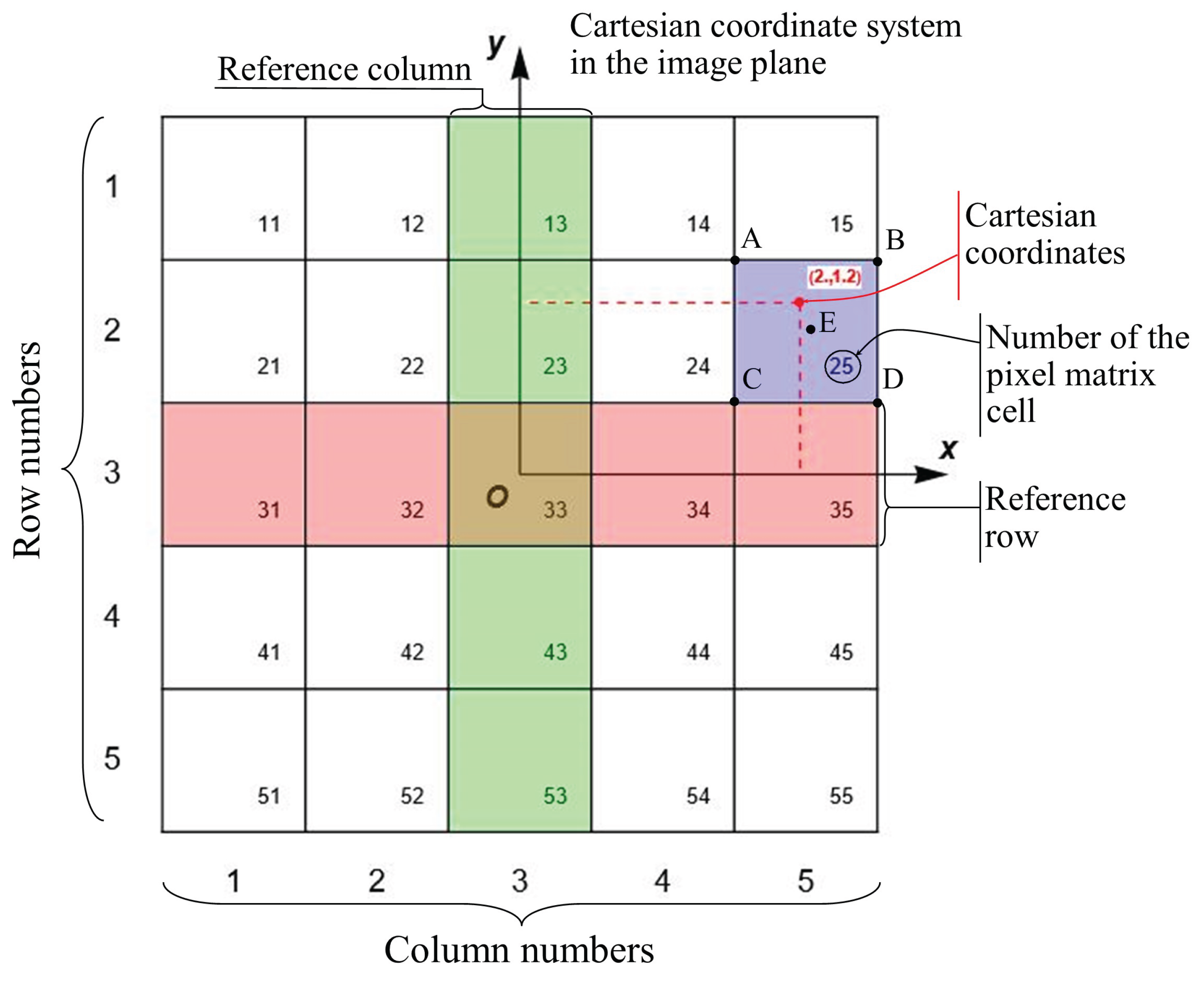
Figure 2.
Bicubic interpolation
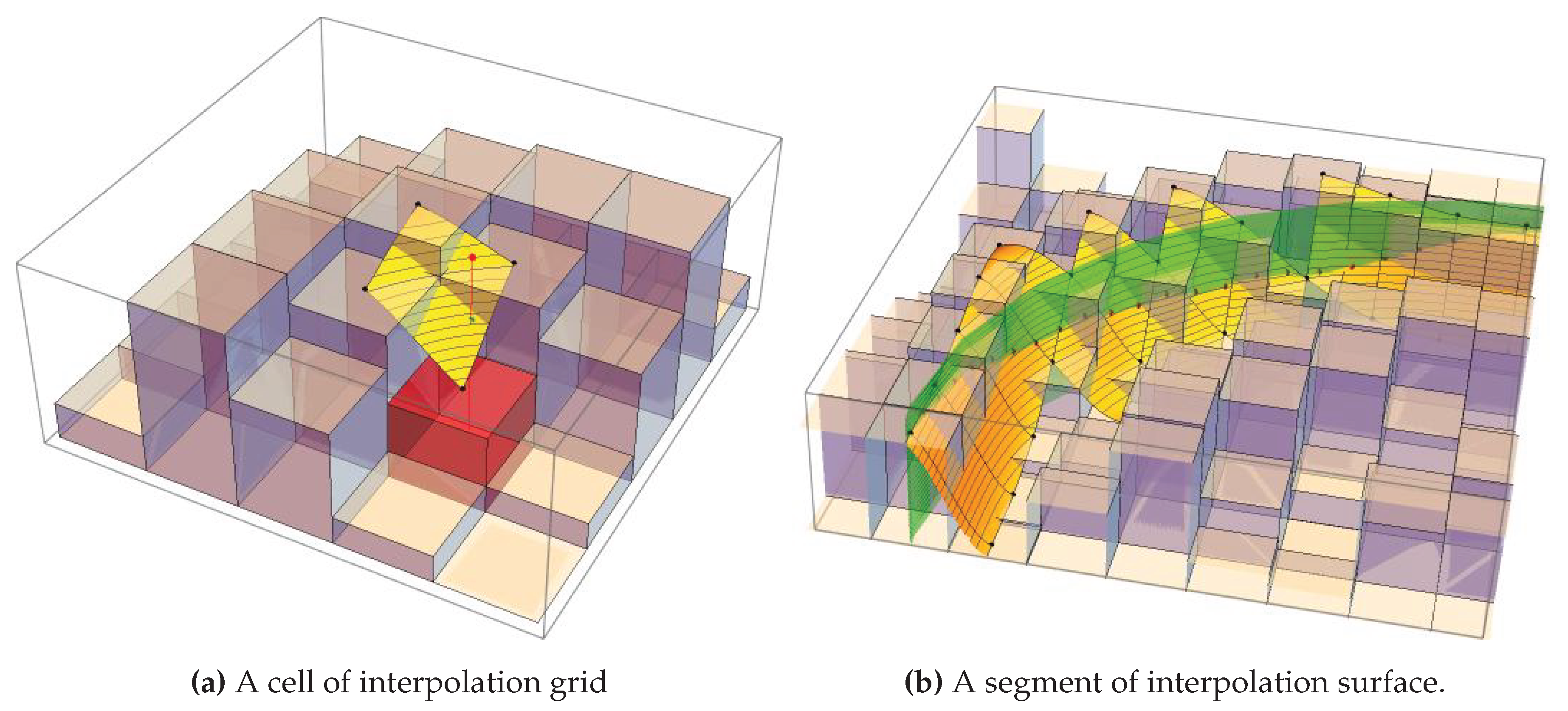
Figure 3.
Schematic of the curve rasterization process using a first-order operator .
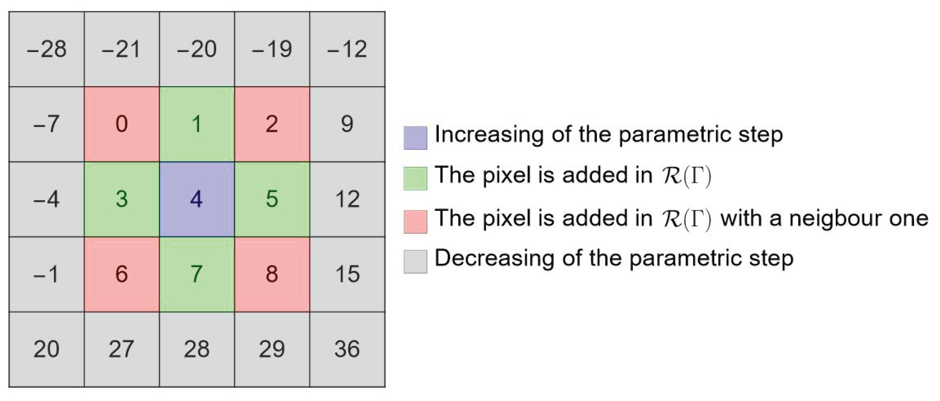
Figure 4.
The 16 discrete configurations classified by the second-order operator (Equation 7). For each configuration, the three consecutive curve pixels (green), (red), and (blue) are shown with arrows indicating the local direction. The shaded blue area illustrates the corresponding region of the strip that needs to be filled. Configurations are grouped: linear motion (), smooth turns (), and return points ().
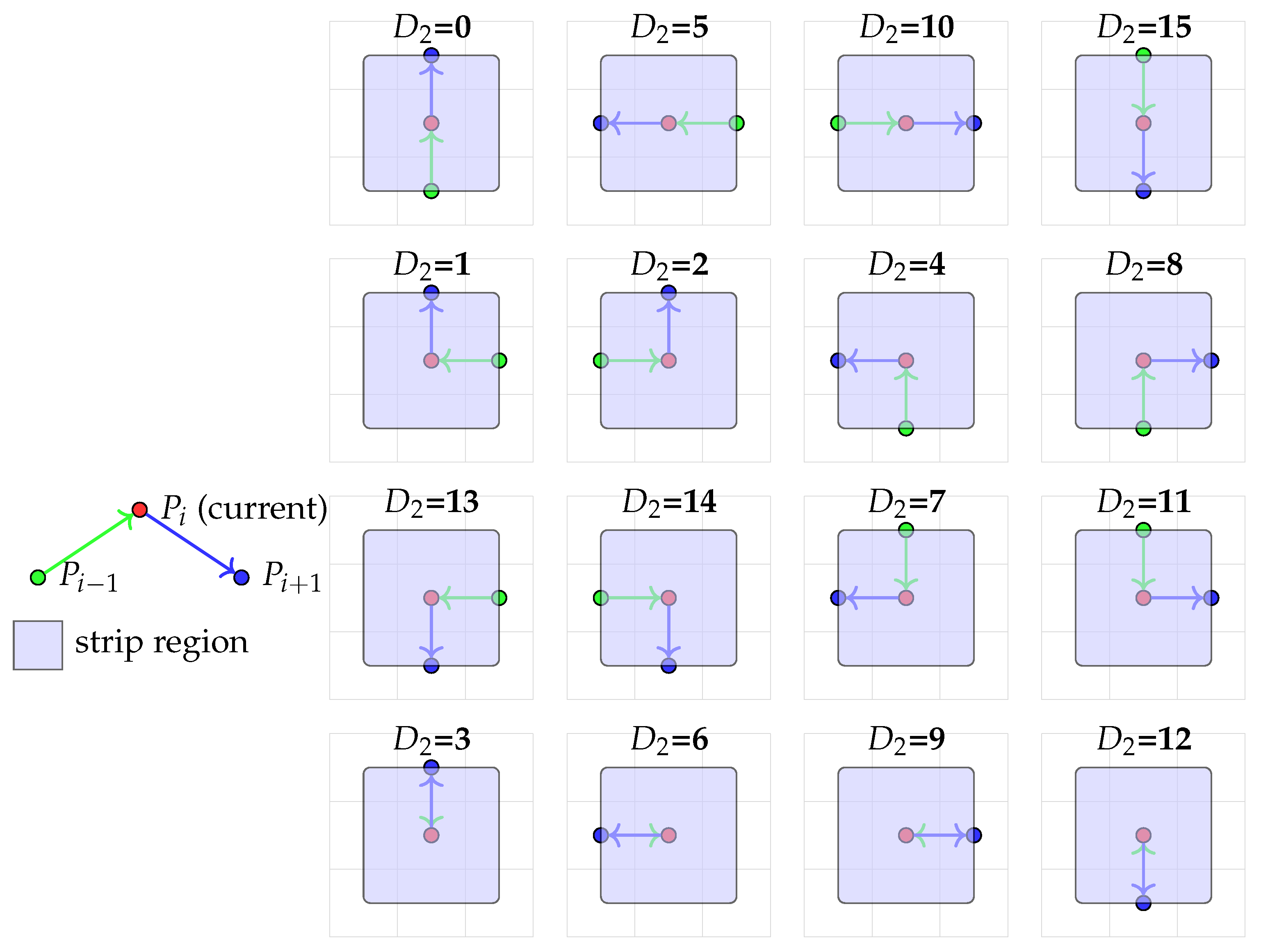
Figure 5.
Geometric correction example.
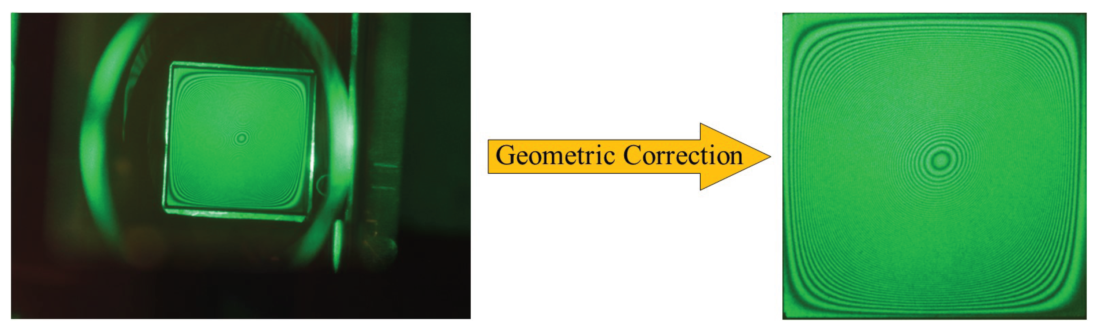
Figure 6.
Flowchart of the complete skeletonization algorithm. Blue boxes indicate preprocessing steps, green boxes represent core algorithmic stages, and orange boxes show the recursive optimization loop. The dashed blue arrow indicates optional iterative filtering-equalization cycles for severe noise cases.
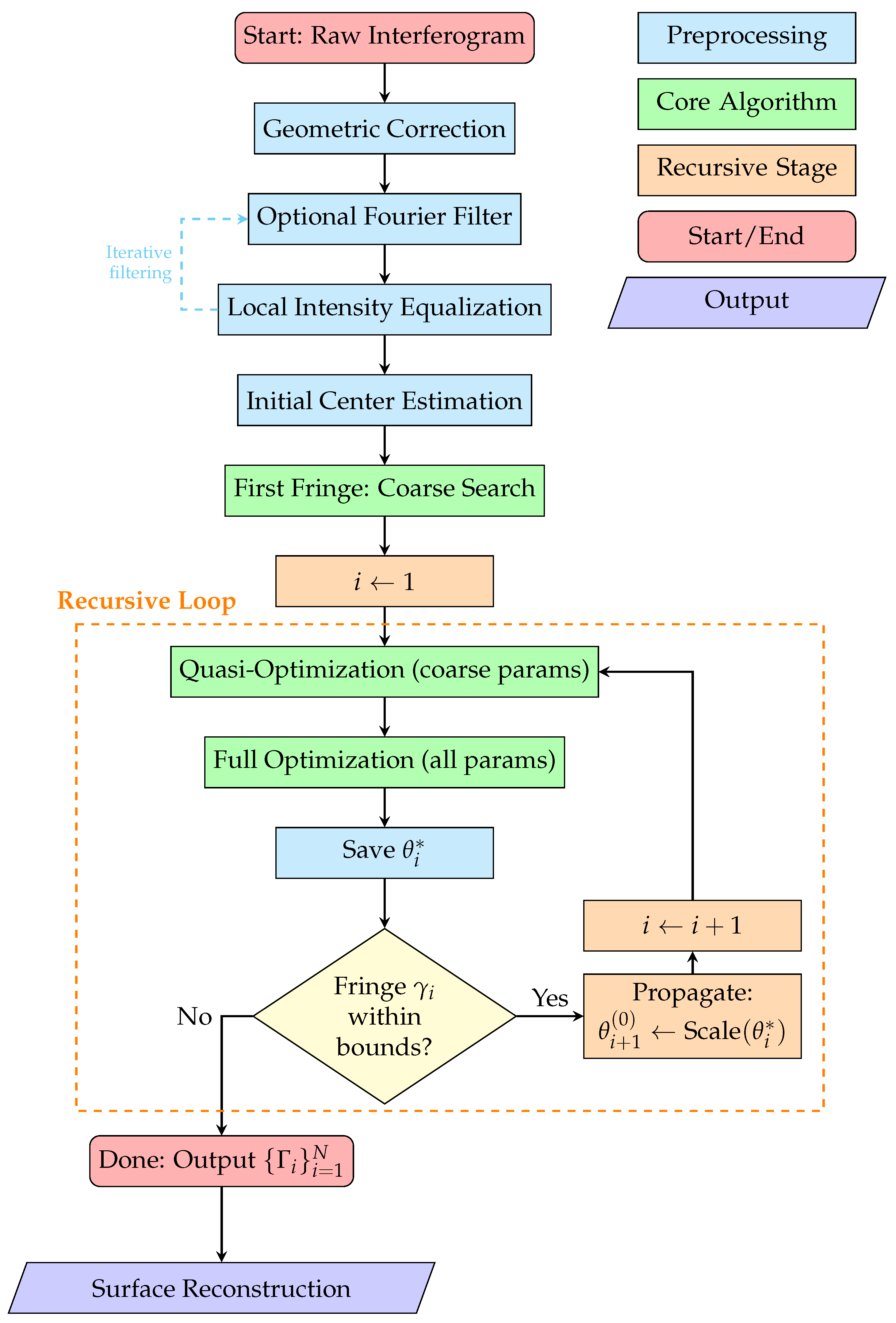
Figure 7.
The preprocessing of a real interferogram. Rows (top to bottom): (a, b, c) original image; (d, e, f) image after Gaussian filtering (blur); (g, h, i) image after intensity equalization. Columns (left to right): (a, d, g) full image; (b, e, h) magnified chosen region; (c, f, i) intensity cross-section, showing the original function (top) and the function after removal of false extrema (bottom).
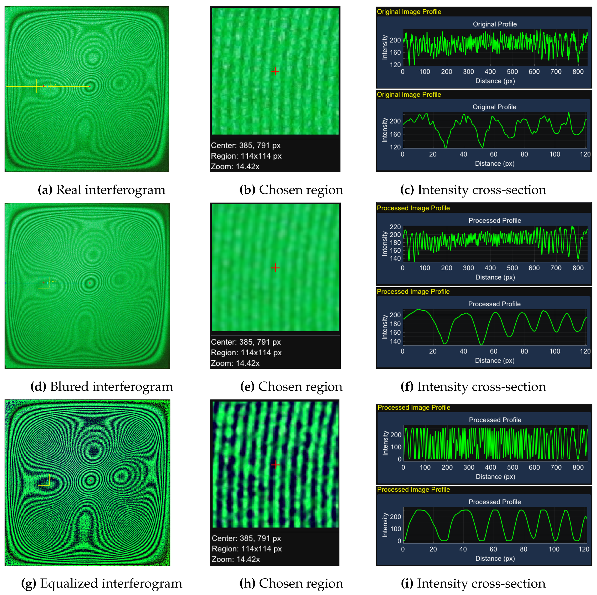
Figure 8.
A Comparison of identification efficiency for different integration methods.
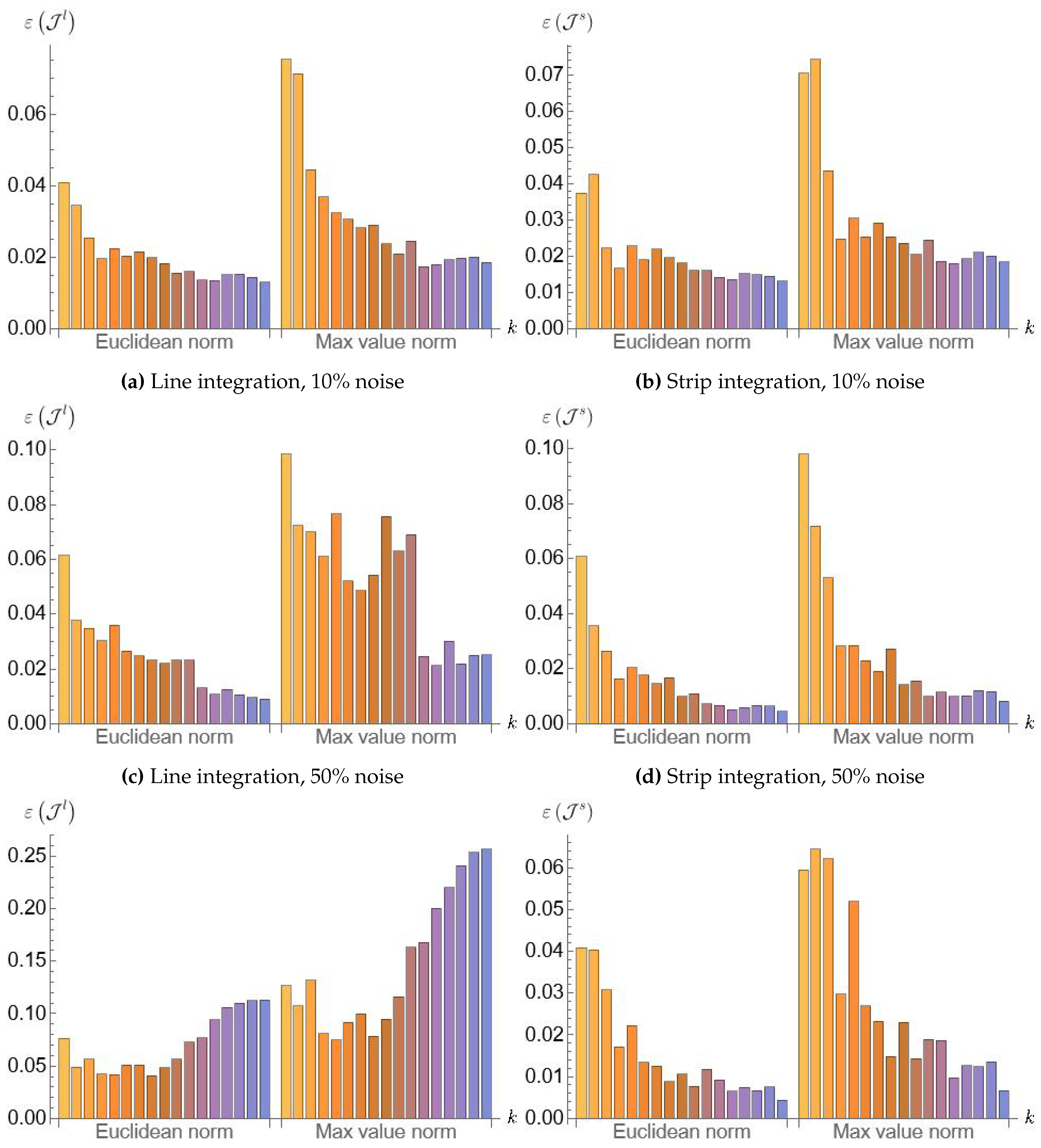
Figure 9.
Fringe identification from synthetic interferogram.
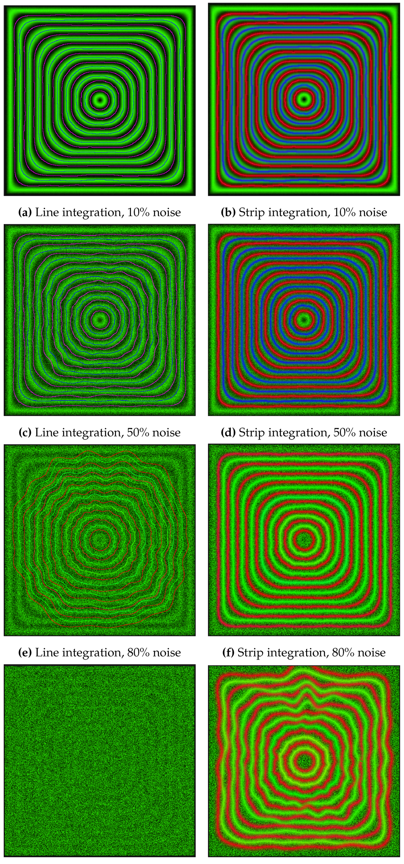
Figure 10.
Validation of the proposed procedure on a real hologram. i) Region of the original hologram. ii) Magnified central region of the processed image. iii) Full processed image, displaying both the identified fringes (red and blue lines) and the intensity-equalized fringe pattern. iv) Deformed surface of the plate obtained from independent theoretical modeling for comparison.
Disclaimer/Publisher’s Note: The statements, opinions and data contained in all publications are solely those of the individual author(s) and contributor(s) and not of MDPI and/or the editor(s). MDPI and/or the editor(s) disclaim responsibility for any injury to people or property resulting from any ideas, methods, instructions or products referred to in the content. |
© 2025 by the authors. Licensee MDPI, Basel, Switzerland. This article is an open access article distributed under the terms and conditions of the Creative Commons Attribution (CC BY) license (http://creativecommons.org/licenses/by/4.0/).
Copyright: This open access article is published under a Creative Commons CC BY 4.0 license, which permit the free download, distribution, and reuse, provided that the author and preprint are cited in any reuse.


