
Submitted:
14 December 2025
Posted:
15 December 2025
You are already at the latest version
Abstract
This study presents a comprehensive analysis of farming-awareness campaigns aimed at enhancing crop pest management through the strategic deployment of infected pests as a biological control mechanism. Additionally, the role of nutrient supplementation is examined within these campaigns to facilitate crop recovery and improve overall agricultural yield. A mathematical model is developed and rigorously analyzed to assess the efficacy of these integrated pest control strategies. The model is investigated with a focus on equilibrium states, stability analysis, and the conditions leading to Hopf bifurcation. Furthermore, optimal control theory is employed to optimize the release of infected pests, ensuring maximum crop yield while maintaining ecological balance. Our study not only underscores the critical influence of nutrient supplementation in augmenting crop productivity but also highlights the risk of excessive nutrient application, which may destabilize the system. These results emphasize the necessity of maintaining an optimal nutrient threshold. By integrating farming-awareness campaigns with precise biological control measures and nutrient management, our study establishes a robust framework for sustainable pest mitigation and agricultural productivity enhancement. The findings suggest that the synergistic application of infected pests and nutrient enrichment not only suppresses pest populations but also enhances crop resilience and productivity.
Keywords:
mathematical model
; crop pests
; equilibria and stability
; hopf bifurcation
; optimal control problem
MSC: 93-10; 34H20
1. Introduction
Crop pests pose a significant challenge for farmers and agricultural producers, as inadequate management can result in reduced yields, lower-quality crops, or even total crop failure [1]. Common pests that damage crops by feeding on leaves, stems, or fruits include aphids, caterpillars, beetles, and moths. The use of biological pest control agents is gaining popularity in both forests and agriculture [3], driven by environmental concerns and advances in biotechnology, which have encouraged a shift away from chemical pest control methods [2]. A key challenge in future pest management lies in the production and application of biological insect control agents. Natural organisms such as bacteria, fungi, viruses, protozoa, and nematodes are considered effective biological pest control agents [4,5]. Among various biological pest control techniques, the strategy of releasing infected pests into agricultural systems is the most effective. In this context, agricultural awareness plays a vital role.
Agricultural awareness campaigns are essential for informing and educating communities about the damage pests inflict on crops and how to protect them while minimizing pesticide use [6]. Pesticide communication initiatives inform farmers about the risks associated with chemical pesticides, encouraging a reduction in their use [8,19]. Those who understand these risks are more likely to adopt alternative pest control methods, such as Integrated Pest Management (IPM) or biopesticides [20,21]. IPM is a crop protection approach that combines various pest control techniques, selecting the most effective strategies for implementation [22,23]. Its main objective is to limit the use of pesticides and other interventions to economically justifiable levels while minimizing risks to human health and the environment [9]. Farm awareness programs are designed to promote the adoption of biocontrol methods for crop pest management [30]. Enhancing farmer awareness helps farmers prevent crop losses while reducing the negative impacts of pesticide use [7].
Mathematical modeling plays a crucial role in analyzing pest control strategies that use infected pests, typically involving viruses as biopesticides. For example, Pathak et al. [26] studied the dynamics of the pest population influenced by viral infection. The application of entomopathogenic fungi such as Beauveria bassiana and Metarhizium anisopliae within integrated pest management programs has been examined by the authors of [34,35]. Furthermore, Silva et al. [18] emphasized the importance of deploying biocontrol agents at optimal times and locations to maximize pest management efficacy while minimizing the environmental impact. Tan and Chen [36] introduced continuous and impulsive pest management techniques, with an emphasis on scenarios involving the lab release of infected insects.
The incorporation of farming awareness into pest control modeling was first introduced by Basir et al. [10], who examined the dynamics of the pest using biopesticides. Building upon this, Abraha et al. [29] proposed a mathematical model that integrates farming awareness, biopesticide application, and optimal control theory, revealing the occurrence of Hopf bifurcation. Recent studies have explored the use of predatory insects as part of farming awareness-based initiatives to better understand crop–pest dynamics [33].
Nutrients, including both macronutrients and micronutrients, play a vital role in supporting the growth and developmental processes of plants [11]. These nutrients are needed in substantial quantities and are integral to numerous biochemical functions vital to plant development and physiology [13,14]. Effective nitrogen management is key to enhancing crop yields and preserving soil fertility [12]. The appropriate application of macronutrients and micronutrients can strengthen plant disease resistance, improve crop quality, and support sustainable agricultural practices [15]. Therefore, by ensuring the proper nutrient supply, crop production can be enhanced [31], but excess amounts of nutrients can have negative effects on the crop yield [37]. Thus, control of nutrient use is required for maximum crop yields.
The studies mentioned above enhance our understanding of the intricate interactions among pests, pathogens, and various management techniques. The findings offer important guidance for designing pest control methods that are not only efficient but also sustainable and ecologically responsible. However, a mathematical model that integrates farming knowledge-based application of infected pests and nutrients remains unexplored. This study aims to develop a mathematical model that captures the dynamics of crop pest populations influenced by the release of infected pests and the application of nutrients within an agricultural setting. In addition, it examines the role of agricultural awareness in shaping the deployment of control measures, including both the release of infected pests and the input of nutrients. To study cost-effectiveness, an optimal control problem is formulated. The Pontryagin Maximum Principle is applied to identify optimal intervention strategies. Through rigorous mathematical and numerical analyses, our study yields valuable insights into effective and sustainable approaches to crop pest management.
The paper is arranged as follows. In the next section, we propose the mathematical model. The mathematical analysis is presented in Section 3. The model with optimal control approach is analyzed in Section 4. Numerical simulations and sensitivity analysis are presented in Section 5. Section 6 concluded the paper with major findings and real-world applications.
2. The Mathematical Model
We propose an eco-epidemic model for pest control, incorporating four dynamic variables to characterize the system, namely, the biomass of crop, , the susceptible pest, , the infected pest, , and level of agricultural awareness, , at any time . The derivation of the mathematical model is based on the following facts.
- H1:
- The logistic growth is assumed for crop biomass with r as the intrinsic growth rate and K as the maximum crop biomass [10,27]. In addition, we consider the impact of nutrients on the quick recovery of crops. Let c be the efficacy of the nutrients to enhance the carrying capacity of crop biomass. The modified carrying capacity of crop biomass due to awareness is [31]. The crop population is consumed by both susceptible pests (S) and infected pests (I) at the rates and , respectively. Here, as the infected pests are weak and will consume the crops at a lower rate [10]. The dynamics of crop biomass is governed by the following equation:
- H2:
- The susceptible pest population increases due to consumption of crop biomass, with a conversion efficiency . However, it decreases due to natural mortality and infection caused by contact with infected pests [10]. Thus, we have the following equation for the susceptible pest population:
- H3:
- Infected pests grow through infection of susceptible pests and interactions with the hosts. Also, the infected pests increase due to additional applications influenced by awareness campaigns. Their population is reduced by natural death and infection-induced mortality. Thus, the dynamics of infected pest population is modeled by the equation below:
- H4:
- The level of agricultural awareness is influenced by various factors. Awareness campaigns increase the level of awareness through media platforms such as social networks and television at a rate . The impact of pest damage also increases awareness, directly proportional to the density of the total population of pests, modeled by the term [10]. Over time, the level of awareness decreases due to inactivity or lack of involvement at a rate . The local awareness rate is the rate at which local awareness is generated or influenced. These factors play a dynamic role in shaping agricultural awareness.
Based on the aforementioned assumptions, we obtain the following mathematical model:
For solving the above model, the initial values of state variables are taken as follows:
Remark 1.
Note that the infected pests are released in the system to make the susceptible pests as they are harmful to crops. The term denotes “awareness-driven release of infected pests”. The term represents the infection rate of susceptible pests when they are in contact with infected pests.
3. Analytical Results
It can be established that the system (4) with the initial condition (5), admits a unique solution [16]. In the following analysis, we identify the equilibrium points of the system and examine their stability properties.
3.1. Existence of Equilibria and Their Stability
We identify five equilibrium points for system (4), as outlined below:
- i)
- The crop- and pest-free equilibrium, ,
- ii)
- The pest-free steady state, . Here, and .
- iii)
-
The susceptible pest-free equilibrium, , whereand is the positive root ofwhere, , andSince , a positive root of (6) exists when Thus the feasibility conditions of are and .
- iv)
- The infected-pest-free equilibrium, , where and is the positive root of the quadratic equation:where, Since , a positive value of exists when , i.e., when
- v)
-
The coexisting equilibrium, , whereand satisfies the quadratic equation:withThe existence of positive roots of equation (9) is addressed in the following proposition.
Proposition 1.
Remark 2.
The susceptible pest-free equilibrium is the most significant for this research. We are controlling the susceptible pest using infected pest release, thus our aim will be to make the system free from susceptible pests.
3.2. Basic Reproduction Number
We define the pest-free equilibrium (DFE) as , where
We choose the infected subsystem as and write it in the next-generation form
where F collects all new infection terms and V collects all other transition terms.
Evaluating the Jacobian matrices at the DFE , we obtain
Thus, the next generation matrix is given by
Hence, the basic reproduction number is the spectral radius of K and is obtained as
3.3. Jacobian Matrix and Characteristic Equation
We denote the model variables as . Now, we rewrite our model system (4) as follows:
The Jacobian matrix is determined as
Usually, is evaluated at an equilibrium point . The characteristic equation of the Jacobian is obtained by:
where I is the identity matrix and are the eigenvalues. Sign of the real parts of the eigenvalues determines the stability of the equilibrium point.
3.4. Stability of Equilibria
We now derive the conditions under which an equilibrium is stable. For this, we require determining the nature of the eigenvalues of the Jacobian matrix at that equilibrium point. An equilibrium point is considered asymptotically stable if all eigenvalues have negative real parts. The following theorem addresses the local stability of the previously identified equilibria.
Theorem 1.
- i)
- The crop- and pest-free steady state, is unstable everywhere.
- ii)
- The pest-free equilibrium is stable when and unstable otherwise.
- iii)
-
The equilibrium point will be stable for the following condition to hold,and the cubic equation is stable according to the R-H criteria that is ,, and
- iv)
- Stability of the equilibrium holds under the following conditions:
- v)
- The following conditions guarantee the stability of the coexisting equilibrium :
Proof.
- i)
-
The Jacobian matrix at the crop- and pest-free steady state, is given byThe matrix gives the following characteristic equation:One eigenvalue of the above matrix is positive, hence the axial equilibrium is unstable.
- ii)
-
At the pest-free steady state, the Jacobian matrix takes the form asThis yields the characteristic equation in as below:Roots of the above equation are obtained as , , and . Clearly, all eigenvalues will be negative whenever the following conditions met:
- iii)
-
We construct the Jacobian matrix for the susceptible pest-free equilibrium aswhere,The equilibrium point is stable if and the cubic equation is stable according to the R-H criteria, that is ,, and
- iv)
-
We determine the Jacobian matrix at infected pest-free equilibrium to be:Here,The matrix yields the characteristic equation as below:Here,Using Routh-Hurwitz criteria, we can conclude that the equilibrium is stable when (13) holds.
- v)
-
At the interior equilibrium point , the Jacobian matrix corresponding to the system (4) takes the following form:Here,We compute the characteristic equation of the matrix as below:The coefficients of (22) are as follows:Applying Routh–Hurwitz criterion on equation (22), we get the conditions for roots with negative real parts as follows:Thus the interior equilibrium is stable if and only if the conditions in (27) are satisfied.
□
3.5. Existence of Hopf-Bifurcation
The stability condition of coexisting equilibrium is established in (27). Let be any parameter of the system (4). Now, we derive the conditions for which Hopf bifurcation can occur when crosses the critical value .
Let be a continuously differentiable function of such that
The following theorem characterizes the occurrence of Hopf bifurcation.
Theorem 2.
The coexisting steady state of the system (4) enters into Hopf-bifurcation at if the following conditions hold:
- (1)
- .
- (2)
- .
Proof.
Occurrence of Hopf bifurcation at requires the existence of a pair of complex eigenvalues, say and , such that and also the following transversality condition is satisfied:
The remaining roots of the characteristic equation (22) should have negative real parts.
In light of condition , the characteristic equation (22) becomes
Let (i=1,2,3,4) be the four roots of equation (30). Also, we assume that and are the pair of purely imaginary roots at . Thus, we have and
Here, implies that .
When and appear as complex conjugates, equation (31) implies that . Alternatively, if the pair consists of real values, then by referencing both (22) and (31), it can be deduced that and . To complete the analysis, the next step is to verify the transversality condition.
Since depends continuously on its roots, an open interval can be identified in which and remain complex conjugates. Within this neighborhood, let their typical representations be given by
Next, we proceed to examine the following transversality condition:
Substituting into (22) and then taking the derivative, we have
Here,
Solving for , we have
if . Thus, the transversality condition for Hopf bifurcation is verified. Consequently, the occurrence of Hopf bifurcation at is confirmed. □
4. The Optimal Control Problem
To determine the optimal strategy for releasing infected pests, we introduce an optimal control problem. Specifically, we define two control variables: (to regulate the release rate of infected pests) and (to regulate the awareness campaigns), which govern the timing and intensity of pest deployment. These controls are assumed to be admissible over the interval , where and denote the initial and final times of intervention, respectively. We introduce the parameter for the control-efficacy which will be regulated by . We also introduce one another control function that regulates the application of nutrients. The admissibility conditions are given by and , ensuring both practicality and biological feasibility. Our aim is to determine the optimal controls and that minimize a given cost functional, achieved by applying Pontryagin’s Maximum Principle [17]. Incorporating these controls leads to the following form of the associated state system:
with initial conditions
The objective function for the minimization problem is formulated as follows:
Our aim in proposing the optimal control problem is to maximize crop yield while minimizing pest damage. The objective function (34) will capture the overall cost of pest management. Specifically, represents the weighting constant associated with the susceptible pests, while denotes the weighting constant linked to the release of infected pests. The term accounts for the cost incurred in introducing infected pests into the crop system. The goal is to determine the optimal controls, , which satisfy the prescribed conditions and minimize the associated costs. Mathematically, we have
subject to the state system (32), where
4.1. Characteristic of the Optimal Control Triplet
According to the Pontryagin Minimum Principle [17], the optimal control problem is governed by a set of necessary conditions. This principle reformulates the optimality conditions into the task of minimizing the Hamiltonian function, . The Hamiltonian is defined as follows:
As stated in [17], the optimal controls and satisfy
Now,
Setting () gives the optimal controls as
In view of the boundedness of the controls, we have
Control is determined as follows:
Thus, is the unique solution of the above equation, projected onto . We numerically find using the iteration method (Newton method).
4.2. The Adjoint System
In accordance with the Pontryagin Minimum Principle [17], the adjoint variables satisfy the following relations:
where i.e., , , etc. Thus, we have
The preceding equations delineate the necessary conditions that both the optimal control functions and the state variables are required to satisfy. According to the Pontryagin Maximum Principle [17], the adjoint variables fulfill the terminal boundary conditions for
In the following theorem, we characterize the optimal system.
Theorem 3.
Assuming the objective function attains its minimum over the admissible set U at the optimal control pair , associated with the coexisting equilibrium point , there exist adjoint variables and that satisfy the system of differential equations (40). The adjoint variables satisfy the boundary conditions: The optimal controls can be expressed through the following functions:
and is the unique solution of the following equation:
projected onto .
Remark 3.
The optimal solution is obtained using the forward–backward sweep method. In this approach, the state system (32) is first integrated forward in time with initial values (33) for the control variables. Subsequently, the adjoint system (40) is integrated backward in time. The control variables in (38) are then updated according to the optimality conditions derived from the problem. For the control , we apply the Newton iteration method, which will work along with forward–backward sweep iterative scheme. The processes of forward integration, backward integration, and control updating are repeated iteratively until convergence is achieved, thereby ensuring that the solution satisfies both the state and adjoint systems as well as the optimality conditions.
5. Numerical Simulations
In this section, we present some numerical results that support the analytical findings discussed earlier. Further, by varying key parameters, we examine the system’s behavior under different conditions. Unless otherwise mentioned in the text, the parameter values used for numerical results are same as in Table 1
5.1. Local Sensitivity for
We derive the basic reproduction number as follows:
with
We compute the sensitivity indices using the following set of parameter values:
with
For this set of parameter values, we have
Hence, . For a parameter p, the normalized sensitivity is defined as
Since , we determine the sensitivity indices as follows:
Substituting the values of parameters, we plot the sensitivity indices in Figure 1. From this analysis, we conclude that the most influential parameters are , , and K, each with elasticity close to , meaning a 10% increase in any of them raises the value of by about 10%. The natural death rate d has a strong negative effect (), while extra mortality rate due to infection () has a moderate negative effect (). Also, we note that the parameters and have less effect on pest-free system.
5.2. Global Sensitivity Analysis
To evaluate the impact of parameter uncertainty on crop production, a global sensitivity analysis based on Partial Rank Correlation Coefficients (PRCCs) is conducted. PRCC is a widely used technique for nonlinear dynamical systems, as it accounts for parameter interdependencies while quantifying their relative influence on the model outputs [38,39,40]. The parameter space is efficiently sampled using Latin Hypercube Sampling. The PRCC results for the crop biomass X are shown in Figure 2 & Figure 3. The carrying capacity (K) and intrinsic growth rate (r) are positively correlated with the crop biomass, whereas the crop consumption rate () and the conversion efficiency of susceptible pests () exhibit negative correlations. Parameters associated with infection dynamics, including , and d, show moderate positive correlations, reflecting their indirect role in reducing pest pressure. The remaining parameters display relatively small PRCC values, indicating a limited direct influence on the crop biomass. This outcome is consistent with Figure 17, which demonstrates that awareness primarily enhance crop production through indirect regulation of pest populations.
5.3. Dynamics Without Optimal Control
Figure 4 illustrates the stability of the pest-free equilibrium , achieved under lower values of the infection rate () and the rate of introduction of infected pests (b). Meanwhile, Figure 5 demonstrates that the infected pest-free equilibrium exists and remains stable when the consumption rate is sufficiently high. Figure 6 shows the stability of susceptible pest-free equilibrium . Solution trajectories converge to the point for higher values of b. Effects of the parameter b on the pest population is shown in Figure 7. Notably, the susceptible pests can be eradicated by the release of infected pests.
Figure 8 illustrates that all populations coexist within the system for different values of the infection rate . For each value of , the system exhibits damped oscillatory behavior before approaching a steady state, indicating that the system remains stable within this parameter range. The transition from stability to sustained oscillations is further confirmed in Figure 9, which shows that a Hopf bifurcation occurs at . Again, we plot the bifurcation diagram with respect to b in Figure 10. The occurrence of Hopf bifurcation at the critical values are confirmed in Figure 11. Figure 12 highlights the influence of the rate of crop biomass consumption by pests on the system dynamics. As the consumption rate increases, the system transitions into oscillatory behavior, indicating that a higher consumption rate can induce periodic oscillations through a Hopf bifurcation. Figure 13 confirms the occurrence of a Hopf bifurcation at the critical value .
Impact of nutrient application is shown in Figure 14. The figure shows that nutrients are useful for quick recovery from pest damage. Additionally, Figure 15 presents a Hopf bifurcation diagram with respect to c, representing the rate of introduction of infected pests. The results suggest that a higher introduction rate is unfavorable for pest control, as it destabilizes the system and increases pest management costs. The impact of local and global farming awareness campaigns on crop production is shown in Figure 16. The figure demonstrates that these control strategies can effectively reduce pest populations and enhance crop biomass, leading to improved crop yields.
5.4. Results from the Optimal Control Problem
The optimal control problem represented by (32), (36) and (38), is formulated as a two-point boundary value problem. The forward–backward sweep method treats the state system as an initial value problem while solving the adjoint system (40) as a boundary value problem. The state system (32) is solved using forward iteration whereas the system (38) is solved through the backward iteration schemes, using the parameter values from Table 1 except:
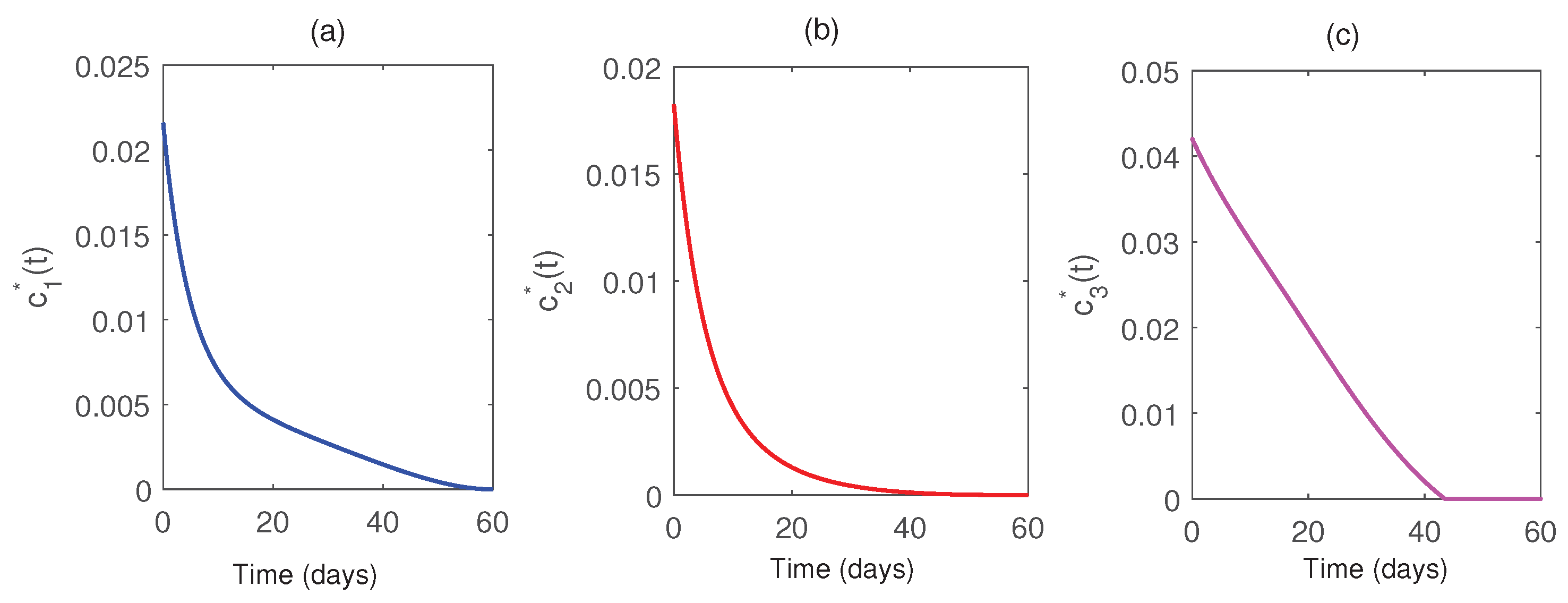
We solve the optimal control problem numerically, and the results are presented graphically in Figs. Figure 17 & Figure 18. These visual representations illustrate the significant impact of the implemented control strategies on the system’s dynamics, demonstrating their effectiveness in optimally suppressing the pest population. The results highlight that a high level of control effort is initially required to achieve substantial pest reduction. However, as time progresses, the necessity of control effort gradually decreases. This strategic approach not only minimizes the costs associated with control implementation but also enhances agricultural productivity. These findings emphasize the dual advantages of cost efficiency and improved yield achieved through optimal control strategies.
5.5. Pest Reduction Ratio, Crop Yield Increase and Control Cost Reduction Rate
The following quantitative metrics are evaluated to compare the baseline (no control) and optimal control scenarios.
- (i)
- Pest Reduction Ratio (PRR): It is defined as follows:
- (ii)
- Crop Yield Increase (CYI): It is defined as follows:
- (iii)
- Control Cost Reduction Rate (CCRR): It is defined as follows:
- (iv)
- Awareness Efficiency (AE): Yield gain per unit awareness cost.
- (v)
- Infected Release Efficiency (IRE): Pest reduction per unit infected-release cost.
Using the parameter values given in Table 1 and (42), we implement the forward–backward sweep method to compute the optimal control trajectories and (as shown in Figure 18) and also compute the results summarized in Table = Table 2.
The results indicate that the optimal control strategy achieves approximately 47% reduction in the susceptible pest population, 22% increase in the crop yield, and 28% reduction in the overall cost compared to the baseline. The efficiency metrics further highlight that awareness campaigns and the release of infected pests contribute significantly to balancing yield improvement and pest suppression.
6. Conclusions
The escalating challenge of managing pest populations poses a significant threat to agricultural productivity, necessitating sustainable and environmentally responsible control strategies. Biological control strategies, which involve the strategic utilization of natural enemies such as predators, parasitoids, and pathogens, offer considerable advantages over conventional chemical pesticides by mitigating environmental contamination and reducing risks to human health. A key approach in biological pest control involves the introduction of infected pests carrying lethal pathogens, which effectively suppresses pest populations while minimizing chemical interventions. By promoting awareness and informed decision-making, the effectiveness of biological control measures can be significantly enhanced. In this study, we investigated a mathematical model that employs natural predators as a biologically sustainable alternative to chemical pesticides for pest regulation. Our model incorporates the interactions between pest populations, their natural predators, and nutrient dynamics within the agricultural ecosystem. Additionally, the model accounts for the influence of agricultural awareness among farmers, highlighting its critical role in optimizing pest management strategies. Furthermore, our study integrates an optimal control framework to evaluate the efficacy of biologically driven pest suppression strategies. The results provide valuable insights into the role of biological control in reducing pest densities, minimizing economic costs, and improving crop yields. The findings underscore the potential of integrating biological control with strategic management interventions to achieve sustainable agricultural practices while mitigating the detrimental effects of pests on crop productivity.
Data Availability Statement
The data used here are mentioned within the article.
Acknowledgments
The authors extend their appreciation to the Deanship of Research and Graduate Studies at King Khalid University for funding this work through the Large Group Project under grant number (RGP.2/58/46).
Conflicts of Interest
The authors declare that they have no competing interests.
References
- Popp, J.; Pető, K.; Nagy, J. Pesticide productivity and food security. A review. Agron. Sustain. Dev. 2013, 33, 243–255. [Google Scholar] [CrossRef]
- Baker, B.P.; Green, T.A.; Loker, A.J. Biological control and integrated pest management in organic and conventional systems. Biological Control 2020, 140, 104095. [Google Scholar] [CrossRef]
- Rajamani, M.; Negi, A. Biopesticides for pest management. Sustainable bioeconomy: Pathways to sustainable development goals 2021, 239–266. [Google Scholar] [CrossRef]
- Bakhtiar, T.; Fitri, I.R.; Hanum, F.; Kusnanto, A. Mathematical model of pest control using different release rates of sterile insects and natural enemies. Mathematics 2022, 10, 883. [Google Scholar] [CrossRef]
- Liu, X.; Cao, A.; Yan, D.; Ouyang, C.; Wang, Q.; Li, Y. Overview of mechanisms and uses of biopesticides. Int. J. Pest Management 2019, 67(1), 65–72. [Google Scholar] [CrossRef]
- Rumble, J.N.; Settle, Q.; Irani, T. Assessing the content of online agricultural awareness campaigns. J. Appl. Commun. 2016, 100(3), 10. [Google Scholar] [CrossRef]
- Raghuvanshi, R.; Ansari, M.A. A study of farmers’ awareness about climate change and adaptation practices in India. Int. J. Agricultural Sciences 2017, 3(6), 154–160. [Google Scholar] [CrossRef]
- Panda, S. Farmer education and household agricultural income in rural India. Int. J. Social Economics 2015, 42(6), 514–529. [Google Scholar] [CrossRef]
- Al Basir, F.; Adhurya, S.; Ray, S. Impact of periodic farming awareness campaign through media for crop pest control management: A mathematical study. In Advances in Mathematical and Computational Modeling of Engineering Systems; CRC Press, 2023; pp. 143–157. [Google Scholar] [CrossRef]
- Al Basir, F.; Banerjee, A.; Ray, S. Role of farming awareness in crop pest management-A mathematical model. J. Teoret. Biol. 2019, 461, 59–67. [Google Scholar] [CrossRef]
- Ali, S.; Riaz, A.; Mamtaz, S.; Haider, H. Nutrients and Crop Production. Current Research in Agriculture and Farming 2023, 4(2), 1–15. [Google Scholar] [CrossRef]
- Nadeem, F.; Hanif, M.A.; Majeed, M.I.; Mushtaq, Z. Role of macronutrients and micronutrients in the growth and development of plants and prevention of deleterious plant diseases-a comprehensive review. International Journal of Chemical and Biochemical Sciences 2018, 13, 31–52. [Google Scholar]
- Shrivastav, P.; Prasad, M.; Singh, T.B.; Yadav, A.; Goyal, D.; Ali, A.; Dantu, P.K. Role of nutrients in plant growth and development; Sources, impacts and management: Contaminants in agriculture, 2020; pp. 43–59. [Google Scholar]
- Pandey, N. Role of plant nutrients in plant growth and physiology. In Plant nutrients and abiotic stress tolerance; Springer Singapore: Singapore, 2018; pp. 51–93. [Google Scholar] [CrossRef]
- Dordas, C. Role of nutrients in controlling plant diseases in sustainable agriculture. A review. Agron. Sustain. Dev. 2008, 28, 33–46. [Google Scholar] [CrossRef]
- Sideris, T.C. Ordinary differential equations and dynamical systems; Atlantis Press: Paris, 2013; Available online: https://link.springer.com/book/10.2991/978-94-6239-021-8.
- Fleming, W. H.; Rishel, R. W. Deterministic and stochastic optimal control; Springer-Verlag: Berlin, 1975. [Google Scholar]
- Silva, C.J.; Torres, D.F.; Venturino, E. Optimal spraying in biological control of pests. Math. Model. Nat. Pheno. 2017, 12, 51–64. [Google Scholar] [CrossRef]
- Tambo, J.A.; Mugambi, I.; Onyango, D.O.; Uzayisenga, B.; Romney, D. Using mass media campaigns to change pesticide use behaviour among smallholder farmers in East Africa. J. Rural Studies 2023, 99, 79–91. [Google Scholar] [CrossRef]
- Remoundou, K.; Brennan, M.; Hart, A.; Frewer, L.J. Pesticide risk perceptions, knowledge, and attitudes of operators, workers, and residents: a review of the literature. Hum. Ecol. Risk Assess. 2014, 20(4), 1113–1138. [Google Scholar] [CrossRef]
- Waichman, A.V.; Eve, E.; da Silva Nina, N.C. Do farmers understand the information displayed on pesticide product labels? A key question to reduce pesticides exposure and risk of poisoning in the Brazilian Amazon. Crop protection 2007, 26, 576–583. [Google Scholar] [CrossRef]
- Way, M.J.; Van Emden, H.F. Integrated pest management in practice—pathways towards successful application. Crop protection 2000, 19, 81–103. [Google Scholar] [CrossRef]
- Karlsson Green, K.; Stenberg, J.A.; Lankinen, A. Making sense of Integrated Pest Management (IPM) in the light of evolution. Evolutionary Applications 2020, 13, 1791–1805. [Google Scholar] [CrossRef]
- Misra, A.K.; Yadav, A.; Bonyah, E. A fractional model for insect management in agricultural fields utilizing biological control. Int. J. Dyn. Control. 13, 1–17. [CrossRef]
- Djouda, B.S.; Ndjomatchoua, F.T.; Moukam Kakmeni, F.M.; Tchawoua, C.; Tonnang, H.E. Understanding biological control with entomopathogenic fungi—Insights from a stochastic pest–pathogen model. Chaos. 2021, 31, 023126. [Google Scholar] [CrossRef] [PubMed]
- Pathak, S.; Maiti, A. Pest control using virus as control agent: A mathematical model. Nonlinear Anal. Model. Control. 2012, 17, 67–90. [Google Scholar] [CrossRef]
- Ghosh, S.; Bhattacharyya, S.; Bhattacharya, D.K. The role of viral infection in pest control: a mathematical study. Bull. Math. Biol. 2007, 69, 2649–2691. [Google Scholar] [CrossRef]
- Al Basir, F.; Chowdhury, J.; Das, S.; Ray, S. Combined impact of predatory insects and bio-pesticide over pest population: Impulsive model-based study. Energy Ecol. Environ. 2022, 7, 173–185. [Google Scholar] [CrossRef]
- Abraha, T.; Al Basir, F.; Obsu, L.L.; Torres, D.F. Pest control using farming awareness: Impact of time delays and optimal use of biopesticides. Chaos Soliton Fractal. 2021, 146, 110869. [Google Scholar] [CrossRef]
- Nyangau, P.; Muriithi, B.; Diiro, G.; Akutse, K.S.; Subramanian, S. Farmers’ knowledge and management practices of cereal, legume and vegetable insect pests, and willingness to pay for biopesticides. Int. J. Pest Manage. 2022, 68, 204–216. [Google Scholar] [CrossRef]
- Basir, F.A.; Venturino, E.; Roy, P.K. Effects of awareness program for controlling mosaic disease in Jatropha curcas plantations. Math. Method. Appl. Sciences 2017, 40, 2441–2453. [Google Scholar] [CrossRef]
- Basir, F.A.; Noor, M.H. A model for pest control using integrated approach: impact of latent and gestation delays. Nonlinear Dynamics 2022, 108(2), 1805–1820. [Google Scholar] [CrossRef]
- Al Basir, F.; Samanta, S.; Tiwari, P.K. Bistability, generalized and zero-Hopf bifurcations in a pest control model with farming awareness. J. Biol. Systems 2023, 31(01), 115–140. [Google Scholar] [CrossRef]
- Bamisile, B.S.; Akutse, K.S.; Siddiqui, J.A; Xu, Y. Model application of entomopathogenic fungi as alternatives to chemical pesticides: Prospects, challenges, and insights for next-generation sustainable agriculture. Frontiers in Plant Science. 2021, 12, 741804. [Google Scholar] [CrossRef]
- Roberts, D.W.; Hajek, A.E. Entomopathogenic fungi as bioinsecticides. In Frontiers in industrial mycology; Springer: Boston, 1992; pp. 144–159. [Google Scholar] [CrossRef]
- Tan, Y.; Chen, L. Modelling approach for biological control of insect pest by releasing infected pest. Chaos Soliton. Fractal. 2009, 39, 304–315. [Google Scholar] [CrossRef]
- Al Basir, F.; Nieto, J.J.; Halder, T.N.; Raezah, A. A. Effects of biopesticides and nutrient in the dynamics of a delay model for awareness-based crop pest control. Int. J. Dynam. Control 2025, 13, 214. [Google Scholar] [CrossRef]
- Reja, S.; Ghosh, S.; Ghosh, I.; Paul, A.; Bhattacharya, S. Investigation and control strategy for canine distemper disease on endangered wild dog species: A model-based approach. SN Appl. Sci. 2022, 4, 176. [Google Scholar] [CrossRef]
- Sarwardi, S.; Reja, S.; Al Basir, F.; Raezah, A.A. Delay-induced bubbling in a harvested plankton–fish model: A study on the role of two fish predators. Nonlinear Dyn. 2025, 113, 22143–22165. [Google Scholar] [CrossRef]
- Marino, S.; Hogue, I.B.; Ray, C.J.; Kirschner, D.E. A methodology for performing global uncertainty and sensitivity analysis in systems biology. J. Theor. Biol. 2008, 254, 178–196. [Google Scholar] [CrossRef] [PubMed]
Figure 1.
Sensitivity indices for using parameter values given in (42).
Figure 1.
Sensitivity indices for using parameter values given in (42).
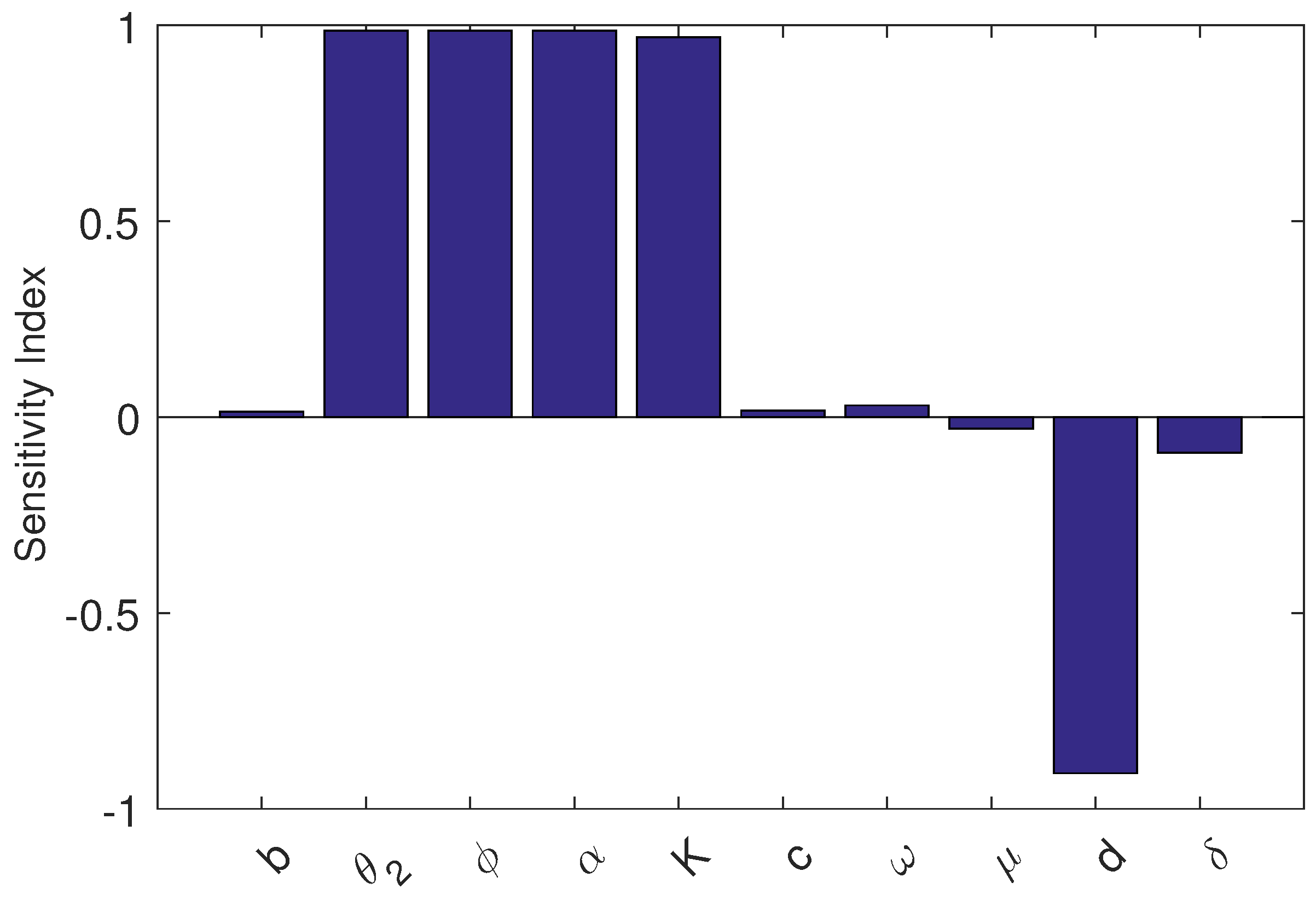
Figure 2.
PRCCs for the crop biomass (X) with respect to the dominant parameters of model (4). The sensitivity analysis is carried out using the Latin Hypercube Sampling (LHS) technique with 1500 realizations. The nominal values of the parameters employed in the analysis are given in Table 1.
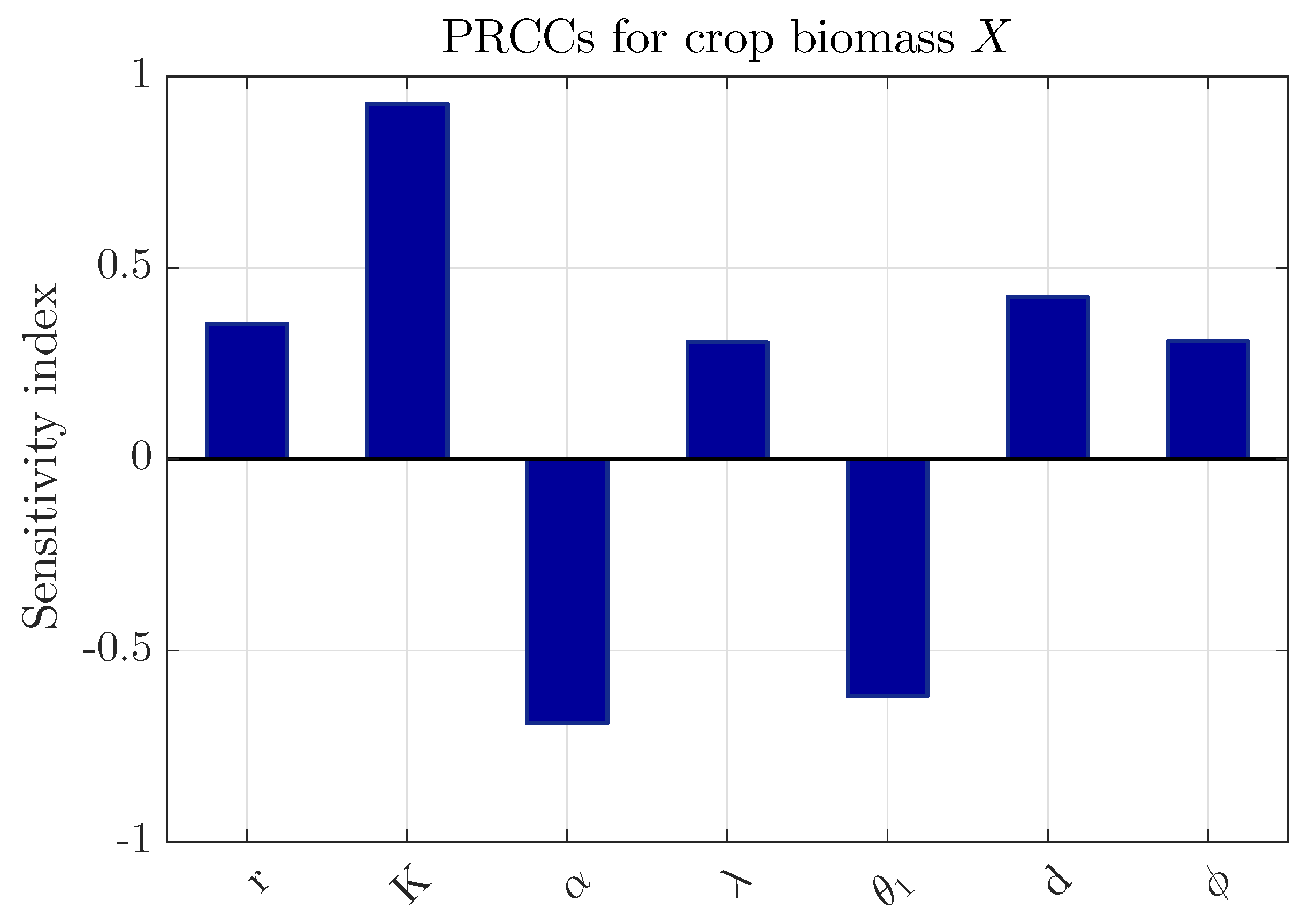
Figure 3.
PRCCs for the crop biomass (X) corresponding to parameters with smaller influence in model 4, displayed on a zoomed scale for clarity. The sensitivity analysis is conducted using the Latin Hypercube Sampling (LHS) technique with 1500 realizations. The nominal parameter values are listed in Table 1.
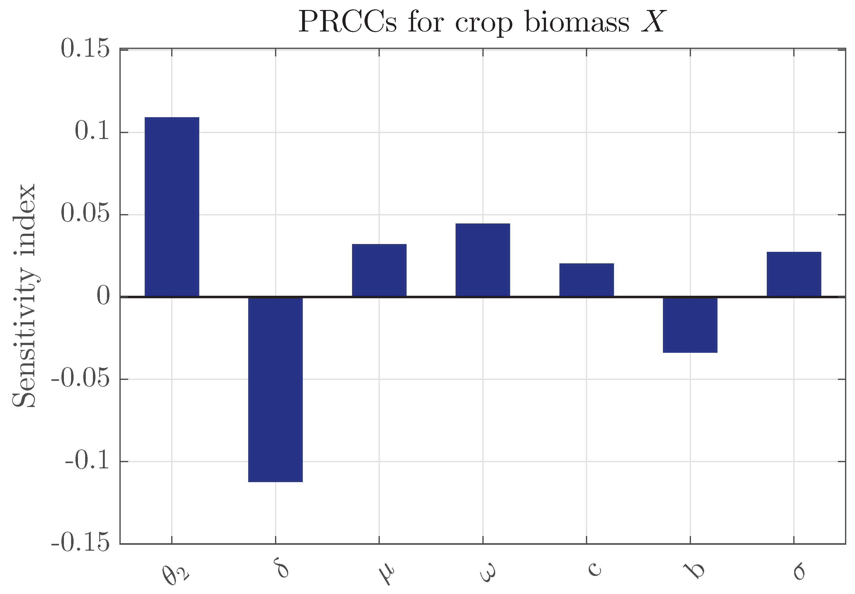
Figure 4.
Solution trajectories of the system (4) for . Other parameter values are taken from Table 1.
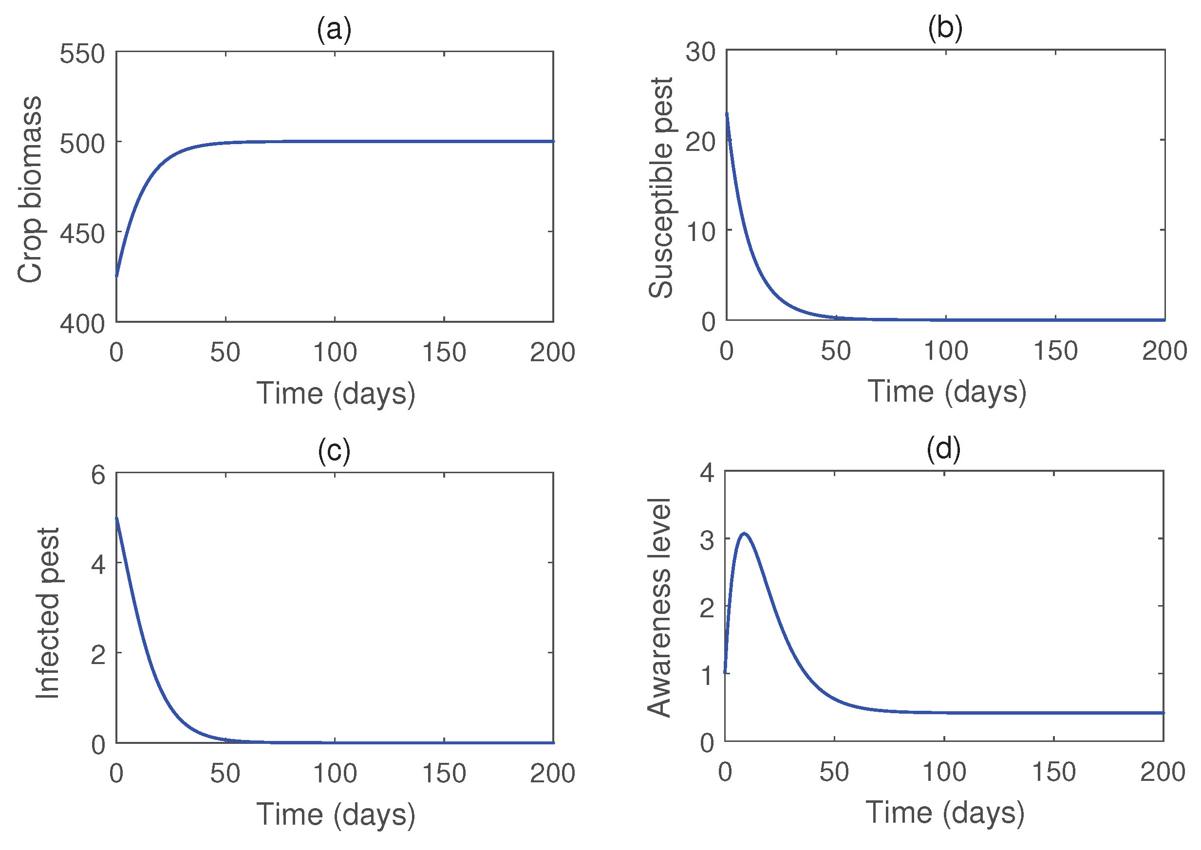
Figure 5.
Numerical solution of the system (4) for . Rest of the parameters have the same value as in Figure 4.
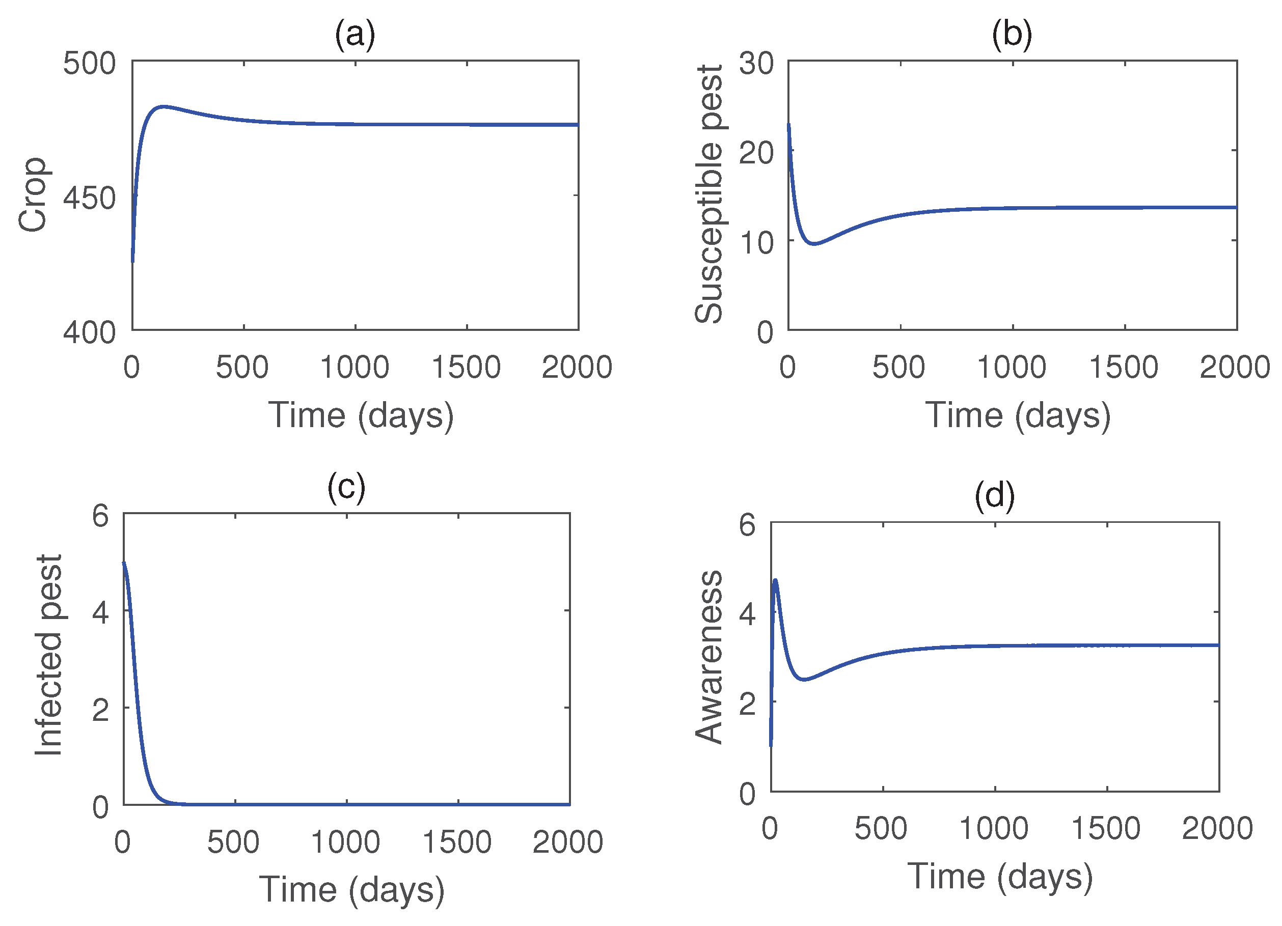
Figure 6.
Time series solutions of the system (4) for two values of b. Parameter values are taken from Table 1 except .
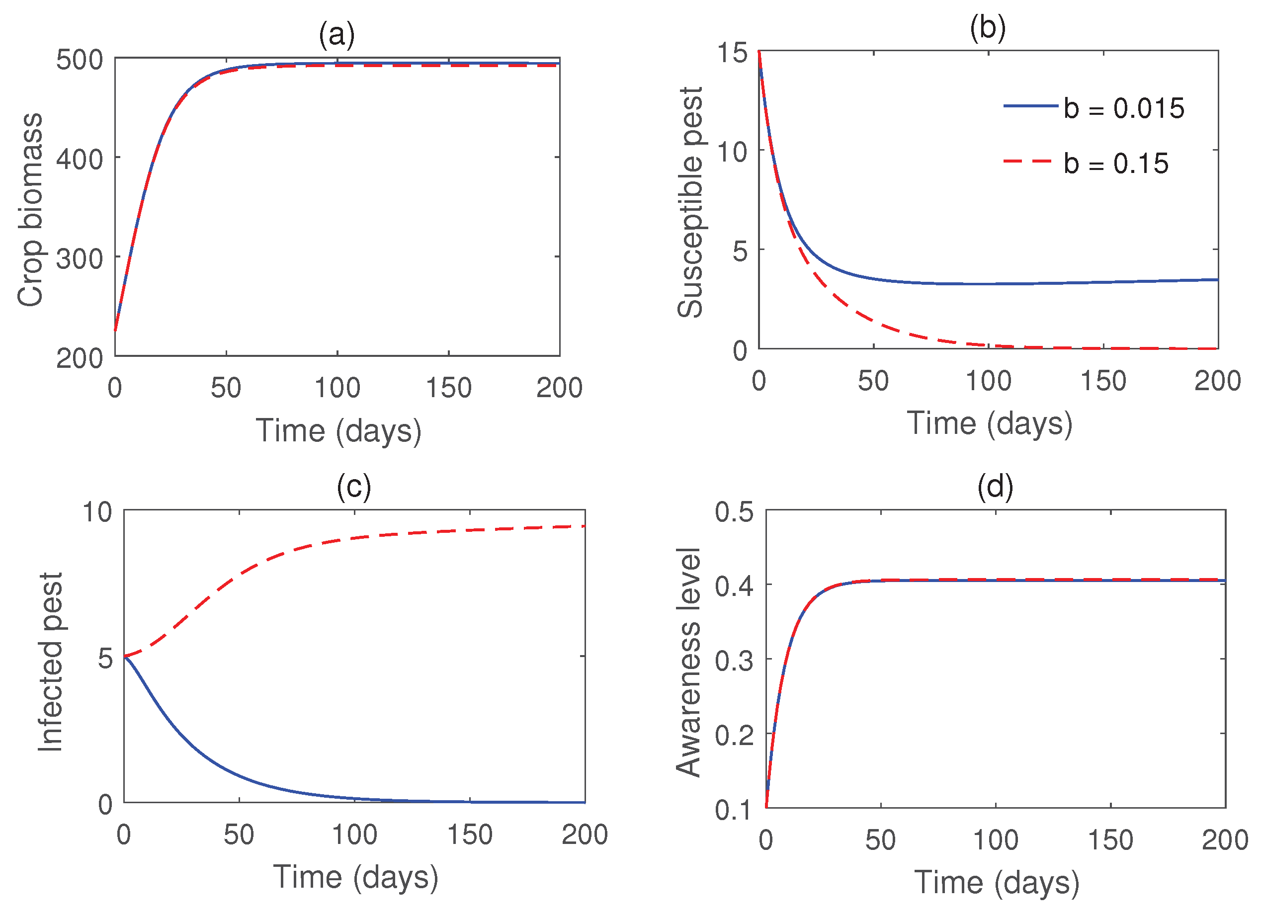
Figure 7.
Impact of the rate of release of infected pests. Parameter values are taken from Figure 6.
Figure 7.
Impact of the rate of release of infected pests. Parameter values are taken from Figure 6.
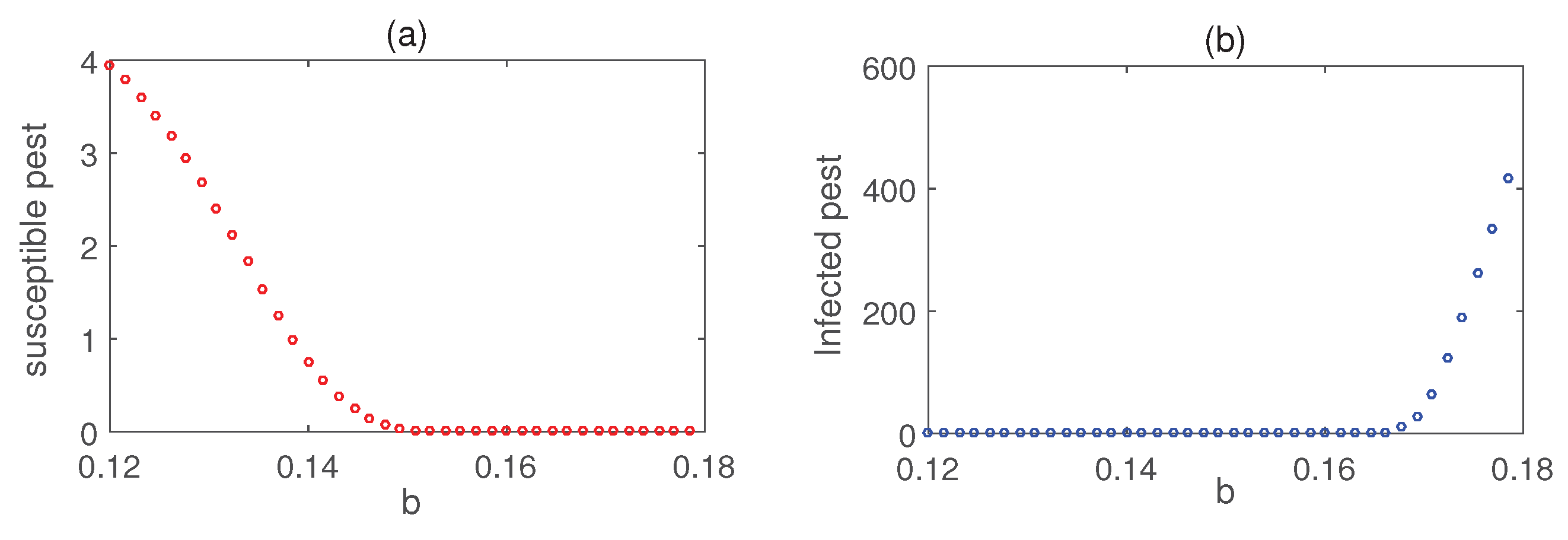
Figure 8.
Time series solutions of the system (4) for different values of . Other parameter values are taken from Table 1.
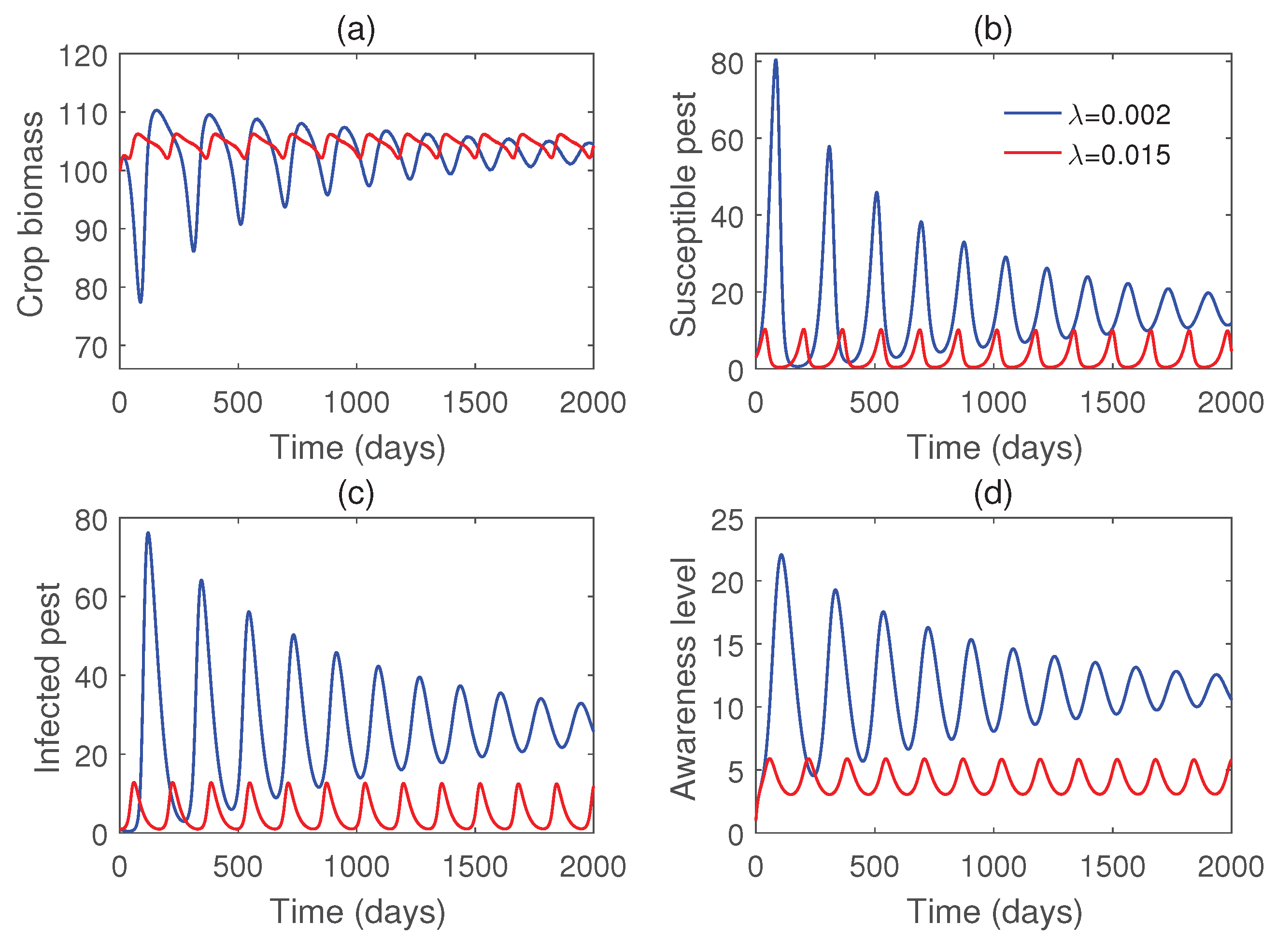
Figure 9.
Bifurcation diagram of system (4) with respect to the parameter . Rest of the parameters have the same value as in Fig. Figure 8.
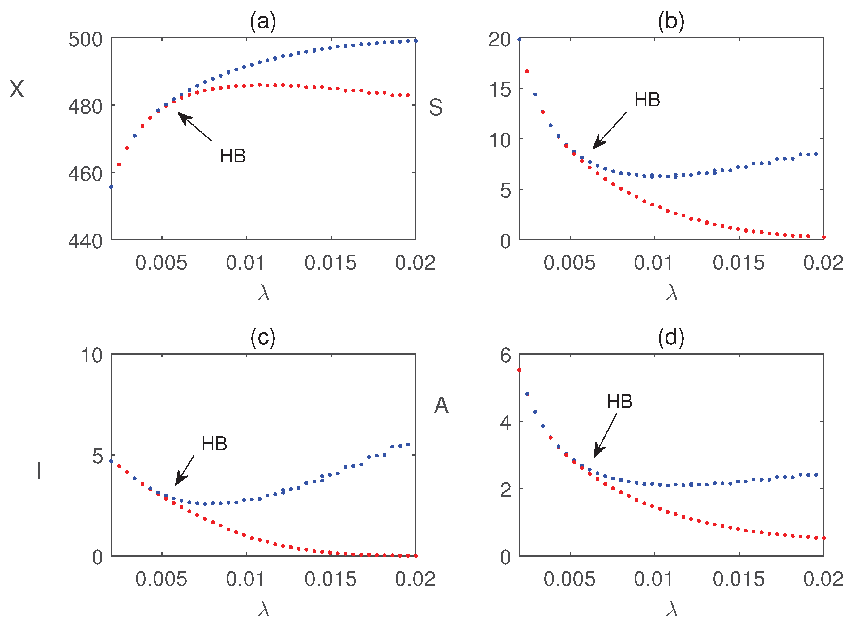
Figure 10.
Bifurcation diagram of system (4) with respect to the parameter b. Other parameter values are taken from Table 1.
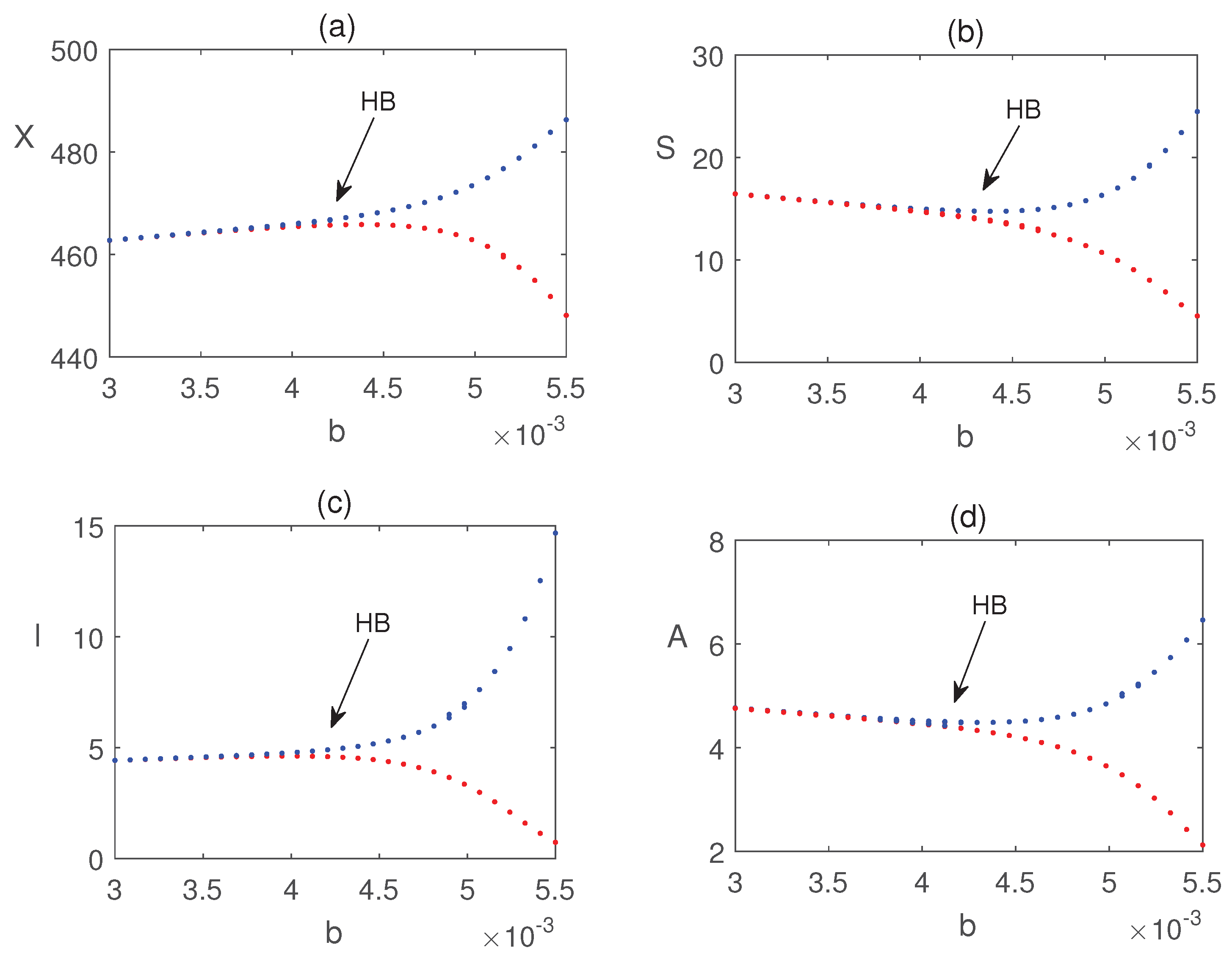
Figure 11.
Plot of with respect to and b. Parameter values are same as in Figure 10.
Figure 11.
Plot of with respect to and b. Parameter values are same as in Figure 10.
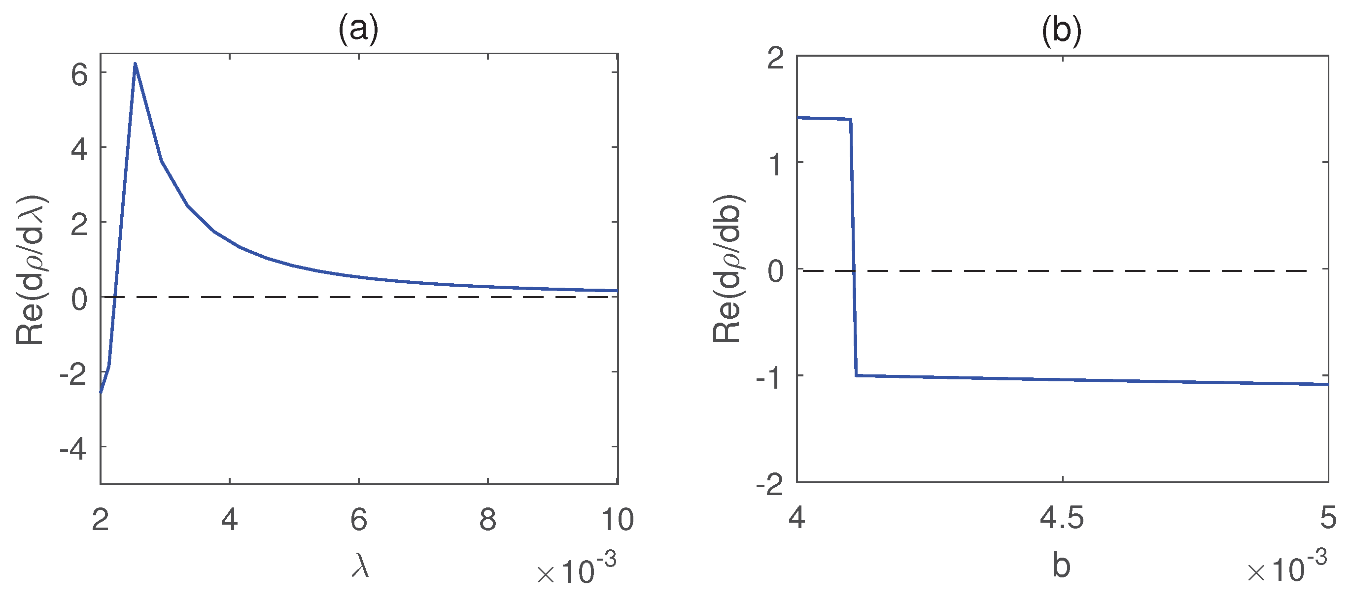
Figure 12.
Numerical solutions of the system (4) for different values of . Rest of the parameters have the same value as in Table 1.
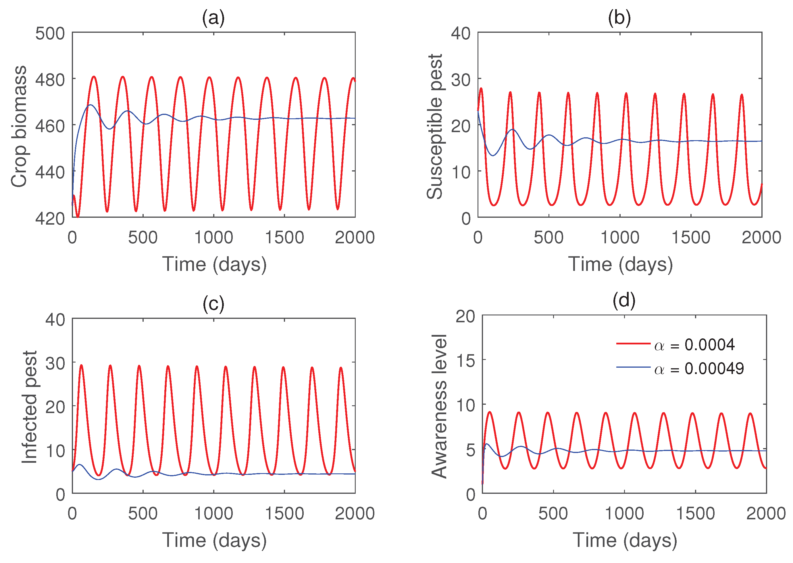
Figure 13.
Bifurcation diagram of system (4) with respect to the parameter . The rest of the parameter values are taken from Fig. Figure 12.
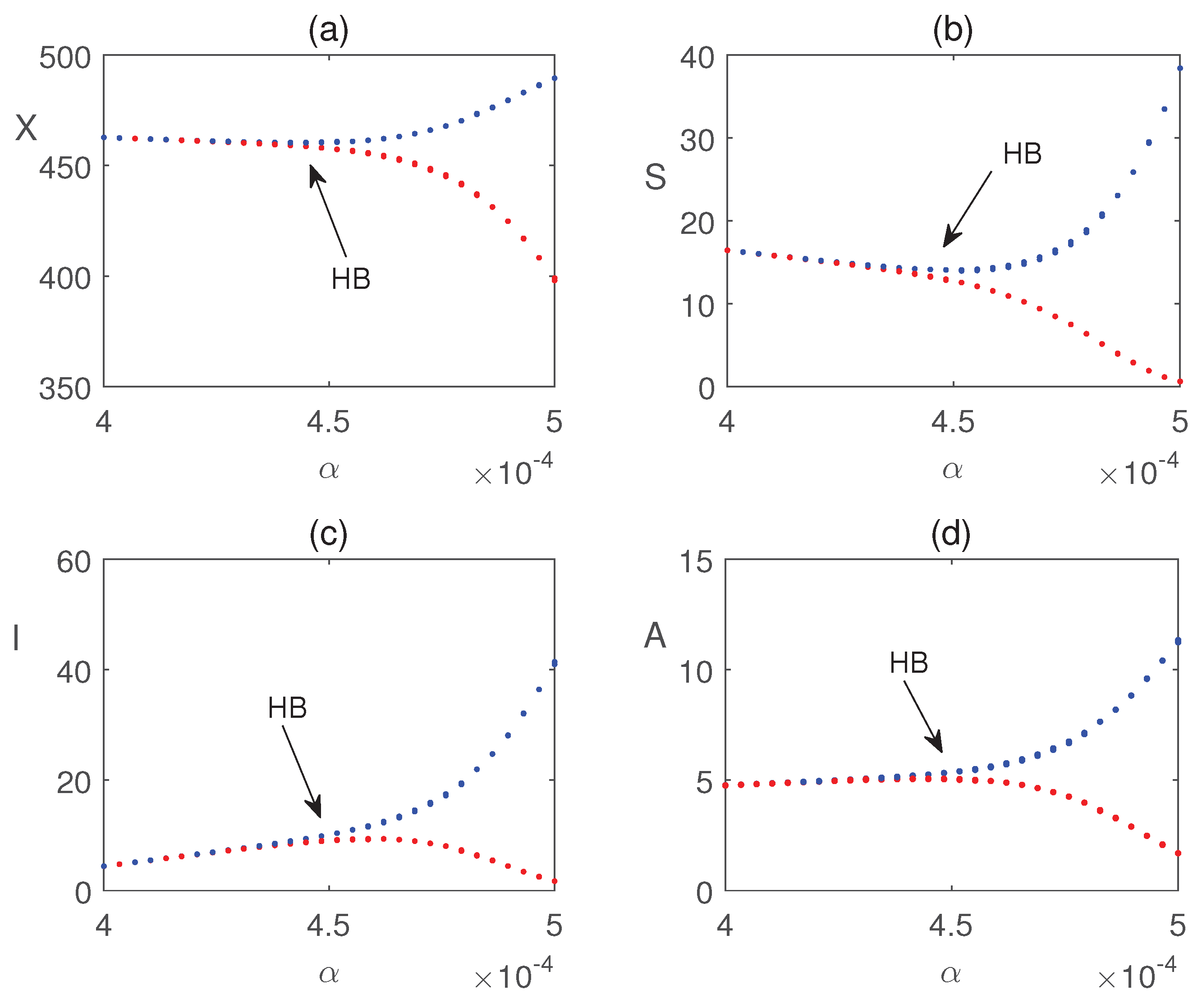
Figure 14.
Effect of nutrients efficacy on the equilibrium values of variables in system (4). Other parameter values are same as in Fig. Figure 10.
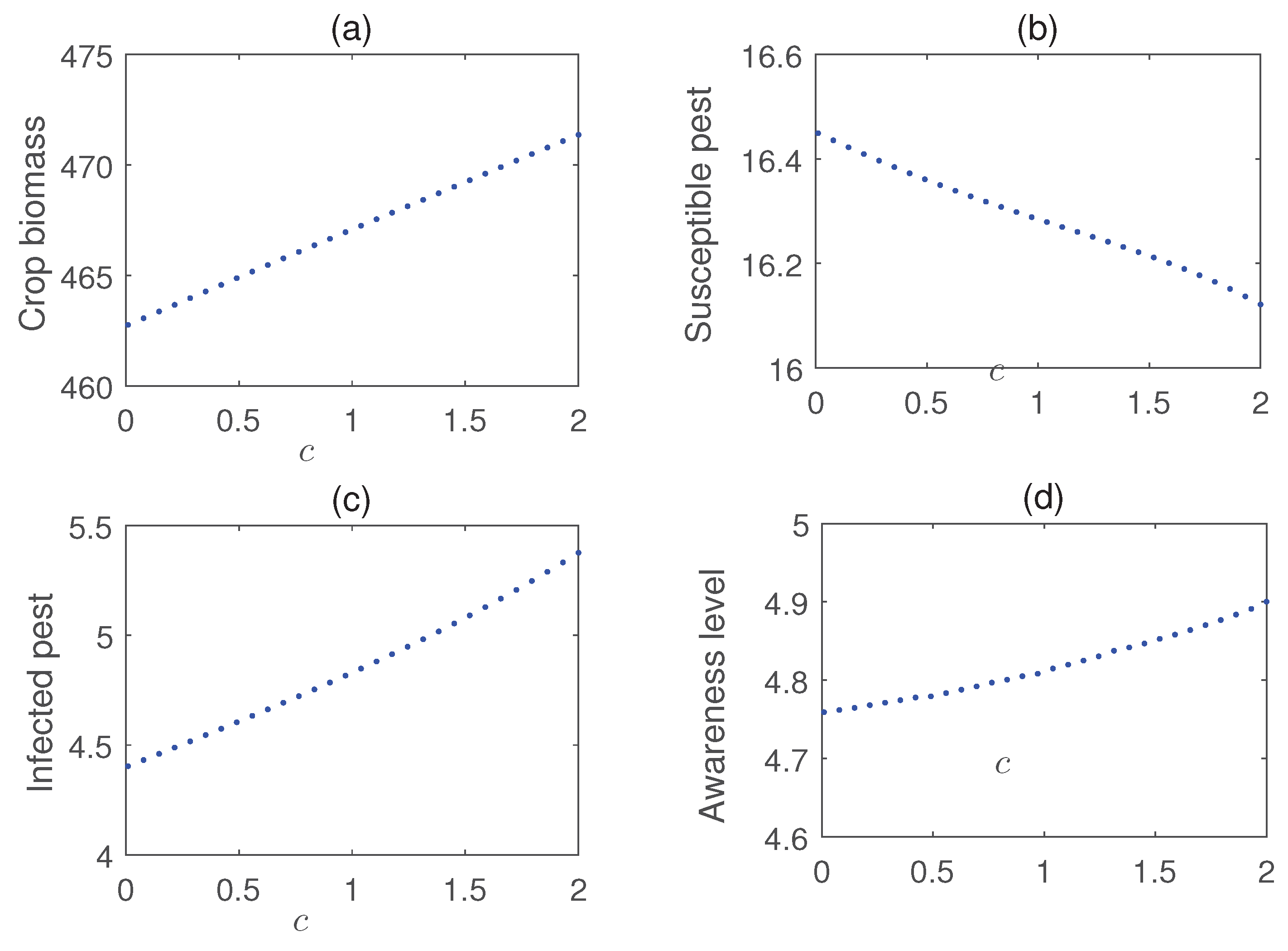
Figure 15.
Bifurcation diagram of system (4) with respect to the parameter c. Other parameter values are same as in Fig. Figure 10.The maximum and minimum values of the periodic solutions are plotted in blue and red dots, respectively.
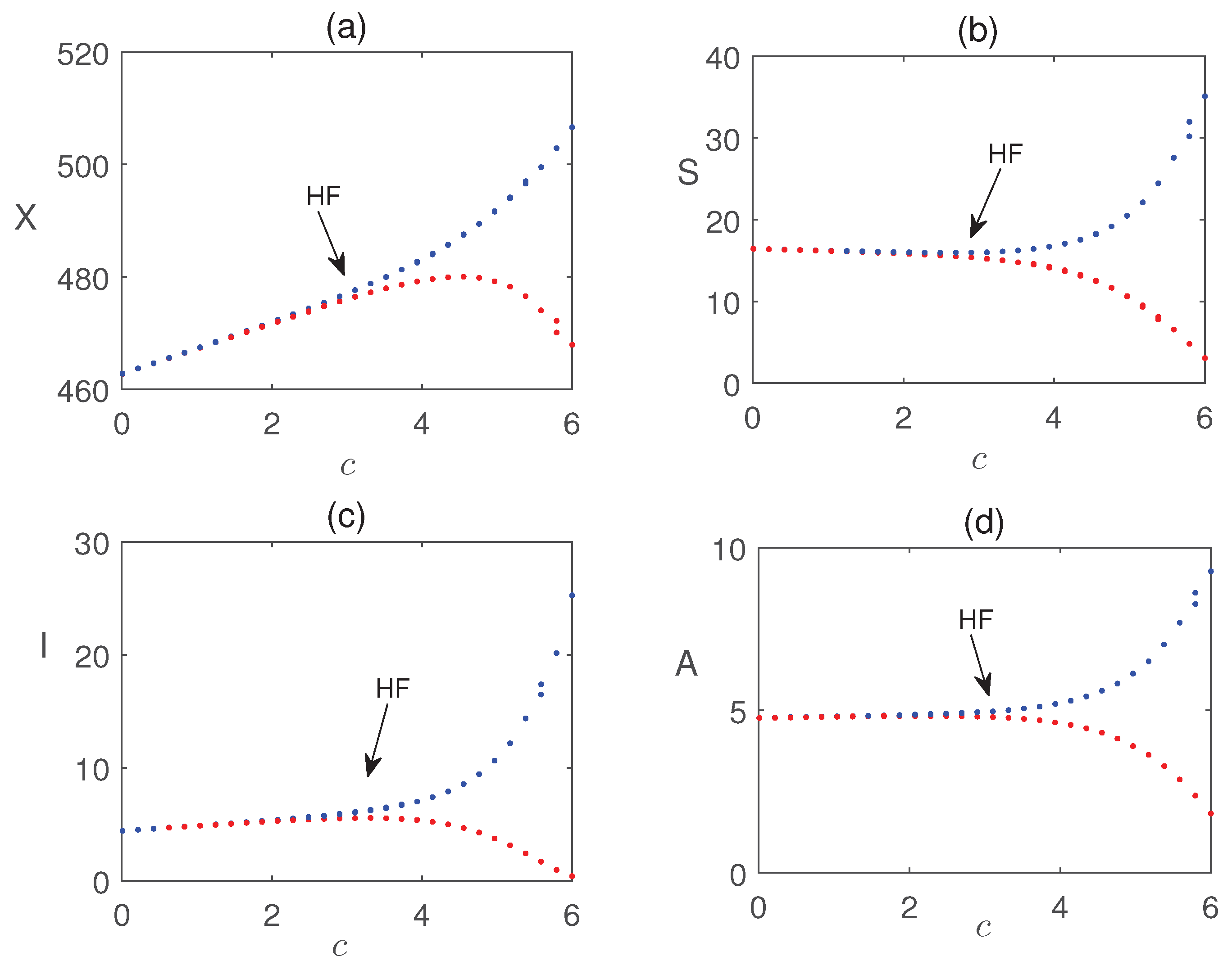
Figure 16.
Combined impacts of the parameters and on the equilibrium values of crop biomass ().
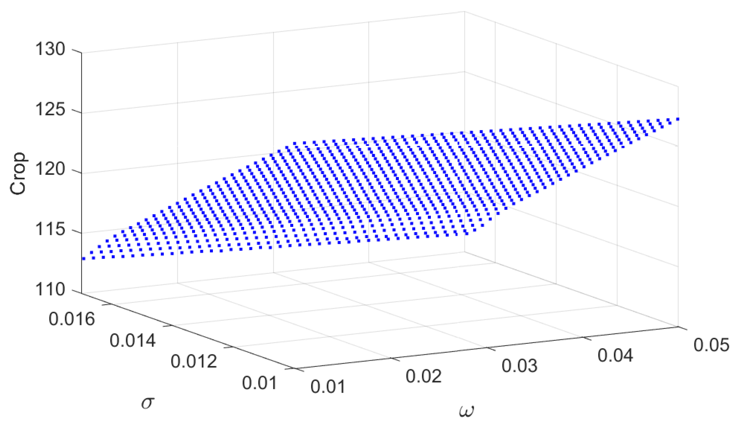
Figure 17.
Simulations of the control system (32) and the system without control (4) for the value of parameters given in Table 1.
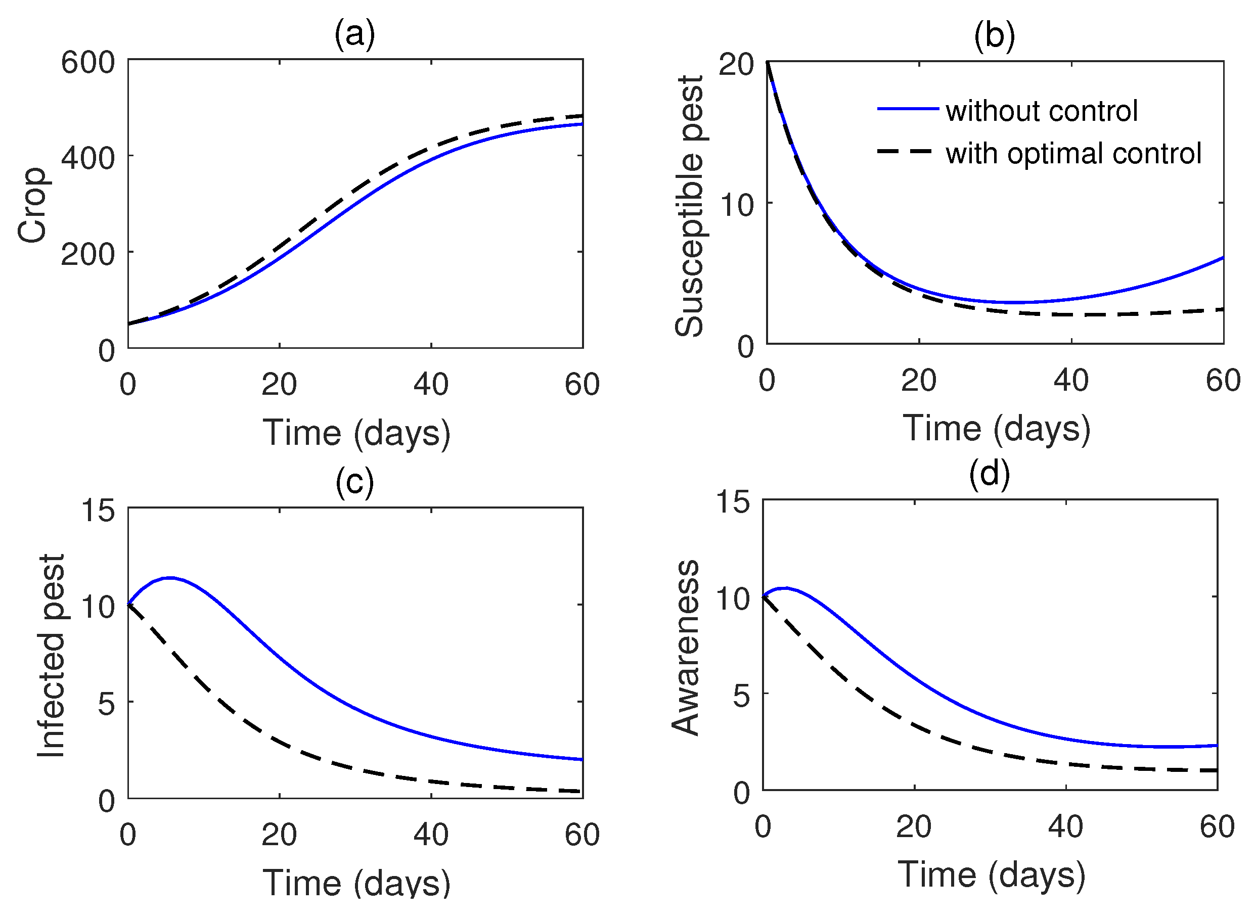
Figure 18.
Plots of the optimal controls with respect to time. Parameter values are same as in Fig. Figure 17.
Figure 18.
Plots of the optimal controls with respect to time. Parameter values are same as in Fig. Figure 17.

| Parameters | Definitions | Values | Units |
|---|---|---|---|
| r | Growth rate of crop biomass | 0.1 | |
| K | Maximum carrying capacity of crop biomass | 500 | g |
| Consumption rate of crop biomass by susceptible pests | 0.0004 | g | |
| Infection rate of susceptible pests by infected pests | 0.0025 | ||
| Conversion efficacy of susceptible pests | 0.6 | — | |
| Conversion efficacy of infected pests | 0.59 | — | |
| d | Natural death rate of pests | 0.1 | |
| Mortality of infected pests due to infection | 0.05 | ||
| Ineffectiveness rate of awareness campaign | 0.12 | ||
| Global awareness campaign rate | 0.05 | ||
| c | Efficacy of nutrient application | 0.01 | g |
| Fraction of nutrient uptake | 0.5 | — | |
| b | Rate of application of infected pests | 0–0.005 | pests |
Table 2.
Comparison of the baseline and optimal control outcomes.
| Scenario | PRR | CYI | CCRR | Control Cost | AE | IRE |
|---|---|---|---|---|---|---|
| Baseline (no control) | – | – | – | 0 | – | – |
| Optimal control | 0.47 | 0.22 | 0.28 | 35.4 | 1.85 | 0.91 |
Disclaimer/Publisher’s Note: The statements, opinions and data contained in all publications are solely those of the individual author(s) and contributor(s) and not of MDPI and/or the editor(s). MDPI and/or the editor(s) disclaim responsibility for any injury to people or property resulting from any ideas, methods, instructions or products referred to in the content. |
© 2025 by the authors. Licensee MDPI, Basel, Switzerland. This article is an open access article distributed under the terms and conditions of the Creative Commons Attribution (CC BY) license (http://creativecommons.org/licenses/by/4.0/).
Copyright: This open access article is published under a Creative Commons CC BY 4.0 license, which permit the free download, distribution, and reuse, provided that the author and preprint are cited in any reuse.


