Submitted:
13 December 2025
Posted:
15 December 2025
You are already at the latest version
Abstract
In this work, we pose and aim to answer the following questions, among others: Which
quantitative characteristics, being satisfied, led to the phase transition from "primordial
soup" to living organisms? How to measure the negentropy of a certain organic matter that
underpinned the appearance of a certain species? To what extent do the biosequences of
living organisms differ from random sequences? How do we quantitatively distinguish
primitive from higher-level organisms? How can we compare the complexity of two living
things? Is there an adequate mathematical structure that naturally and appropriately
represents each organism biosequence and all of them as a whole? What are the properties
of that structure? How does that structure evolve, and what are the theoretical limits of any
further evolution? Is it likely that these bounds will be reached, and what are the "limits of
life?" How to estimate the effect on the mechanism of evolution of natural selection vs. the
one of chance and mutations? To this end, we introduce relevant mathematical structures
and use them for modeling purposes. Finally, we also speculate on possible scenarios of
the origin of life, evolution, and related issues.
Keywords:
string
; bipartite graph
; tree
; monotone path
; local maximum
; helix
; entropy/negentropy
; biosequence
; random sequence
1. Introduction
The origin of life and evolution are foremost issues in science and worldview. Numerous theories about life formation have been proposed since ancient times till today, from various versions of divine creation, to Aristotle’s spontaneous generation, primordial soup origin, and out of the Earth dawning. Darwin’s evolutionary theory was followed by a variety of modifications and modern alternatives which attempt to explain life progression. Occasionally, scientific discussions among different schools include bitter and harsh arguments, without reaching answers satisfying all parties. Often, a new theory that is initially widely admired, a few decades later is criticized and neglected. To a great extent, this is natural: biology is not an exact (in the sense of quantitative, or mathematical) science; therefore, exact (or fully correct) answers cannot be expected. Moreover, we believe that for questions concerning the origin of life and the evolutionary process, developing a fully precise theory is largely impossible.
For example, the simple question at first glance of when life originated on Earth seems to be impossible to answer. The oldest known fossils are approximately 3.7 billion years old, but hypotheses exist that primitive living organisms may have existed nearly 4.1 billion years ago. Understandably, time estimations with a possible error of several hundred million of years look somewhat disquieting. Moreover, even if that above conjecture would be correct, it may not be justifiable because any traces may have disappeared due to various possible catastrophic events that may had arisen any evidence.
By similar reasons a precise theory about life formation looks largely impossible to develop. There is a solid list of requirements for a scientific theory to be acceptable, and most of them look unfeasible to achieve. For example, testing the theory through experimentation and observation may not be possible, since experiments cannot be performed under the Earth’s surface conditions which had been present a few billions of years ago and which are to a great extent unknown. Note that sometimes it could be difficult to provide fully convincing answers even to questions about very recent or ongoing events. For example, there are several quite diverse theories about the origin of Covid 19 pandemic - from an infected bat sold on Wuhan’s marked, to infected raccoon dogs, or bamboo rats, or civets, to leakage from Wuhan’s bio-laboratory. Some experts believe that the reason for the infection will never be found. And all this, provided that the pandemic was witnessed by all the world and Covid 19 is still around.
In view of the obvious difficulties to fabricate a theory of origin of life and evolution satisfying all criteria for a reasonable scientific theory, we believe that for such a theory most important is to meet the following norms:
- -
- The conjectured scenarios must be hypothetically possible;
- -
- The stated suppositions must agree with the available facts and evidences;
- -
- The hypotheses must be to a great degree a product of logical thinking, rather than a result of digging for fossils and presenting a theory based on the partial evidences obtained.
While the first two norms are typical for all natural sciences, the third one is most quintessential for mathematics. In recent decades the use of mathematics and computer science in biological research is becoming increasingly crucial and decisive. Disciplines like mathematical biology, theoretical biology, computational biology, and bioinformatics were established. A substantial body of literature was developed on pertaining topics. Mathematical models helped shedding light on various questions, typically related to the study of diverse living organisms and the processes that rule their anatomy, spread, and behavior.
In the present work we ask and try to answer some important questions related to the origin of life and the evolution. The principal among these are the following.
- -
- Which quantitative characteristics, being satisfied, led to phase transition from “primordial soup" to living organisms?
- -
- How to measure the negentropy1 of the constituents of the primordial soup?
- -
- How to measure the negentropy that fed the appearance of a certain species?
- -
- How to measure the negentropy of a group of organisms and of all living things?
- -
- To what extent do the biosequences of living organisms differ from random sequences?
- -
- How do the introduced quantitative parameters distinguish primitive from higher level organisms?
- -
- How to compare the complexity of two living things?
- -
- Is there an adequate mathematical structure which naturally and adequately represents each organism biosequence and all of them as a whole? What are the properties of that structure?
- -
- How does that structure evolve and what are the theoretical limits of any further evolution?
- -
- Is it likely these bounds will be reached? What are the “limits of life"?
- -
- How to estimate the effect on the mechanism of evolution of natural selection vs. the one of chance and mutations?
- -
- What are the likely scenarios of origin of life and of evolution?
Some of these questions were posed and deliberated in [6,7,8] by introducing appropriate mathematical constructs and performing relevant experiments. Typically, problems involving biosequences are approached using combinatorial techniques such as combinatorial pattern matching and combinatorics on words. Instead, we use geometric techniques in an attempt to address questions like those listed above.2 A key point of our approach is string geometrization which we have applied to biosequences. In the present work we build on our former results by introducing new concepts and further scrutinization of the matter.
In the following section we introduce notions and notations to be used in the sequel. In Section 3, we first recall some definitions related to string geometrization and related properties. Then we define new concepts such as discrete irregular helix, monotone graph, negentropy of monotone path and monotone graph, and we study the properties of some of the introduced structures. In Section 4, we define DNA Spatial Hyper-network and discuss how one can apply the proposed mathematical developments to that network. In Section 5, we contemplate the negentropy of species, of groups of species, and of the DNA Spatial Hyper-network. In Section 6, we speculate on distinction between biosequences and random sequences, borders of life in terms of some of the introduced parameters, the gradient between primitive and biologically complex organisms, and related questions. In Section 7, we share our viewpoint on origin of life, evolution of species, and a Global Life Network as alternative to Tree of Life. We also debate about certain related questions of philosophical flavor. We conclude with some final remarks and proposals for future work in Section 8.
Throughout, key conclusions and postulations are highlighted and indented for better comprehensibility. Some theoretical results related to string geometrization were stated in [6,8] without proof. We provide the corresponding proofs in Appendix A. In Appendix B we include a figure and three tables summing up some results of our former experiments.
2. Notions and Notation
2.1. General
By we denote the cardinality of a set X and by the straight line segment with endpoints x and y. By we denote the Euclidean distance between points x and y, and by the distance between point x and set Y.
Given a list T of nonnegative real numbers (not all of which equal 0), a normalization of T is obtained by multiplying each value in T by , where
Given an approximation algorithm A for a minimization problem with a set of instances , let be the value of an approximate solution on instance found by A. The approximation ratio of A on I is , where is the optimal solution for I; the worst case performance ratio of A is . We will say that an algorithm with performance ratio r finds an r-approximation to the optimal solution. For more details the reader is referred to [13,22].
2.2. Notions of Theory of Words
The theory of words studies the structural properties of strings composed from letters of a given alphabet, and provides algorithms for solving diverse problems defined on strings. Among the most important motivations for the discipline is its relevance to computational biology, and more precisely, to the automated analysis of biosequences. This includes a great variety of problems whose portrayal is beyond the purposes of the present paper. Some avenues of the ongoing research are surveyed in [2,3,4,5,14,39,54].
In the literature, the terms word, sequence, and string are often used interchangeably. A sequence is often defined in mathematics as a function whose domain consists of a set of consecutive integers, and a string over X, where X is a finite set, is often defined as a finite sequence s of elements from X (X is also sometimes called the alphabet). The term word is frequently used as an abstraction of the other two terms. In biology, the prevalent term is biosequence; biosequences are built from the four letters A, T, C, G, and have finite length.
Below, we recall a few basic notions and fix some notations to be used in this paper.
In string over set X, is the term of s (), which is some element of X. The number of elements in s is called the length of s and denoted . If , we say that s is the empty string, denoted by . We denote consecutive repetitions of term x in string s by .
A of a string s is obtained by selecting some or all consecutive elements of s. More formally, a string v is a substring of the string s if there are strings u and w such that (where we may have or ).
2.3. Notions of Graph Theory
Let be a simple graph, i.e., with no multiple edges between any pair of vertices and with no loops (edges that connect a vertex to itself). A simple path in G is a sequence of vertices of G such that no vertex is repeated. A shortest path between two vertices of G is a simple path of a minimum length (number of edges) connecting the vertices. A simple cycle is a closed simple path. G is triangle-free if contains no triangle, i.e., a cycle of length 3. G is connected if there is a path of edges of G between any two of its vertices. G is sparse if , otherwise it is dense. The chromatic number of G is the minimum number of colors sufficient to color the vertices of G, so that any two adjacent vertices are colored by different colors. G is 2-colorable (or 2-chromatic) if its chromatic number is 2. G is bipartite if its vertices can be divided into two parts, such that the graph edges can connect vertices only from different parts but not from the same part.
Graph G is geometric if its vertices are points of and its edges are segments containing graph vertices. A geometric graph G is rectilinear if each edge of G is a straight line segment, which is parallel to a coordinate axis.
A graph is called directed if its edges have directions. A directed path in a directed graph is a sequence of vertices such that for each vertex v in the sequence there is a directed edge pointing to a successor of v in the sequence. A directed graph is connected if there is a directed path between any two vertices. A directed graph is strongly connected if for any pair of vertices u, v there is a directed path from u to v and a directed path from v to u.
3. Theoretical Background: String Geometrization, Monotone Paths, Monotone Graphs, and Negentropy
3.1. Monotone Paths
In order to make the paper self-contained, in this section we first recall some basic definitions and related properties from [6,7,8]. Then we extend those considerations by introducing new structures and concepts to be used in biosequence interpretation.
Let be the origin of the Cartesian coordinate system. A monotone path in is a sequence of points (nodes) connected by segments which are unit edges of the rectangular grid, where the coordinates of any point , , are pairwise greater than or equal to the corresponding coordinates of any preceding point.
Let be a monotone path of length m. We define the maximum deviation from linearity of L as
and average deviation from linearity of L as
If for every node p of L, the voxel centered around p intersects the line segment , we call L a linear path. In the degenerate case where a monotone path is aligned with one of the coordinate axes, L is called inline path.
It is easy to see that the following facts hold:
Fact 1.
Given a point , there is at least one linear path from θ to p.
Fact 2.
If L is a linear path from θ to p, then .
Remark 1.
Note that when (which is the case for biosequences), the and of a linear string are at most 1.
The third characteristic of a string s will be called the number of local maxima of s and denoted . Formally, by a local maximum we mean a point for which is greater than and . However, regarding the usual applications of extrema of discrete functions, in particular in view of our own purposes, counting all such maxima does not seem to be very relevant. Instead, local maxima can be counted only if they “stand out" compared to other, “indistinguishable" local extrema, which differ very little from neighboring points. Thus, we adopt the notion of number of local maxima as “method dependent." Specifically, our choice of method is the one provided by [58].
Let be a point in . Denote by the set of all monotone discrete paths between and p. It is easy to see that the following holds.
Fact 3.
.
Each path consists of points, with initial point and terminal point p. Now let be the set of all monotone paths of length m. Then we have
Fact 4.
, where .
3.2. String Geometrization
Let be a string on an alphabet . We inductively construct an ordered set of points corresponding to string s as follows.
Let be the element of for . If for some j, , then we set . Thus, we obtain a monotone discrete path associated with the string s.
With a reference to formulas (1) and (2), we can define and average deviation from linearity of s as and . We call slinear string if its corresponding monotone path is linear. If is inline, then s is an inline string.
Now denote by the greatest attained by a permutation of string s, i.e.,
The following theorem (stated in [6] without proof) will be used in Section 4 in the deliberation on “borders of life". The proof of the theorem is given in Appendix A.
Theorem 1.
Given a string s over an alphabet in which letter appears times, ,
where P is the set of all partitions of into two disjoint, nonempty sets N and Z.
If is a partition for which is attained, then for every permutation of s whose corresponding discrete monotone path contains the point , where if and if , .
Remark 2.
Given a string s of length m, the numbers of appearances of the letters can be counted with operations. Once this is done, can be computed in time, i.e., the overall solution of the considered problem takes time. While this is exponential for an unbounded n, for a fixed n — as in the case of biosequences — the computation time is linear in the string length.
3.3. Relation to Minimum Enclosing Cylinder
Our definition of a linear string refers to a discrete monotone path whose voxels intersect the line segment between the initial and terminal points. Respectively, deviation from linearity refers to the distances from the points of the monotone path to that line segment.
Another possible approach is to consider a straight line that minimizes the maximal distance over all points of , which is the axis of the minimum enclosing cylinder for the set . Note that while in two dimensions the problem of finding the minimum enclosing cylinder can efficiently be solved in linear time, it is not so in higher dimensions. Even in 3D, the available exact algorithms take super-cubic time (see, e.g., [1,12,18]). This makes the problem practically intractable for strings of considerable size, e.g., like the biosequences we investigate in the following sections. The following theorem demonstrates that the deviation from linearity which we adopt is no more than twice greater than the one defined by the minimum enclosing cylinder. Moreover, the computation of the former requires only a linear number of operations for a fixed dimension n (4 in the case of biosequences), and is therefore without a doubt advantageous from a computational complexity perspective. Note also that in the course of our experiments, we measured a significant difference between the deviation from linearity of biosequences and random sequences; thus, a minimum enclosing cylinder approach – provided that one could afford to wait for the solution – would provide no advantage in distinguishing biosequences from random sequences aside from changing the magnitude of distinction by at most a factor of 2.
Theorem 2.
Let be a monotone discrete path of length at least 3. A 2-approximation to a minimum enclosing cylinder for L can be found with operations.
The proof is given in Appendix A.
3.4. Monotone Path and Irregular Discrete Helix
The monotone paths introduced and discussed in the previous sections can be regarded as irregular discrete helices. Figure 1 gives examples of two monotone paths in . The one on the left resembles a discrete analog of a standard cylindrical helix, which is known as triangular helix or regular skew-apeirogon. The one on the right features a similar (although irregular) helical structure, which we call irregular discrete helix. Clearly, in dimensions higher than three relevant illustrations are not possible. In dimension four, one can obtain certain evidence by viewing the projections of the monotone path on the four coordinate planes.
3.5. Negentropy of a Monotone Path
Broadly speaking, the term “negentropy" (short from “negative entropy") is interpreted as a trend towards creation, maintenance, and increasing the order within a system. For this, “free energy" is utilized (which, according to the theory of thermodynamics, is energy available to perform work). In biology, negentropy hints at the capability of living organisms to create, maintain, and increase their internal order and complexity by utilizing free energy from the environment through metabolism and adaptation (thus resisting against the second law of thermodynamics).
For the purpose of ease of adding the probabilities of independent events, the entropy is customarily defined as a logarithmic function. Likewise, given a monotone path L, we can define the negentropy of L as
or, alternatively, as
We have , as if and only if L is an inline path.
In turn, given a string s, its negentropy is
Let be a set of strings and the set of the corresponding monotone paths. Then the total negentropy of is
Note that the logarithmic function is strictly monotone, therefore both and (as well as ) are fairly good for comparative analysis of strings. Thus, as an alternative, one can measure the negentropy of a monotone path L by its maximum (or average) deviation from linearity. As in the definition using a logarithmic function, (resp. ) if and only if L is an inline path.
3.6. Monotone Graphs
Let be a set of monotone paths in , , and let be their union. can be regarded as a geometric graph, called monotone graph with vertices – the nodes of the paths, and edges – the grid edges of the paths in .
The monotone paths of are subgraphs of . If we assign directions on the edges of a path starting from the origin, we obtain a directed path with first vertex at the origin. Taking the directed paths for all , we obtain a directed graph .
3.6.1. Properties of and
Property 1.
is connected. is connected but not strongly connected and has no directed cycles.
Property 2.
In and all simple monotone paths between any two vertices have the same length.
Property 3.
and are rectilinear. By Property 2, all cycles of are of even length. Hence, is bipartite and 2-chromatic.
Property 4.
and are sparse. (The proof is given in Appendix A.)
Property 5.
is triangle-free (follows from Property 3).
Note:It is known [20] that a triangle-free graph with sufficiently many edges (e.g., of the order of ) is bipartite, otherwise it may be non-bipartite. Monotone graphs are always bipartite, regardless their low density.
Property 6.
Both in and one can find a shortest path from the origin to any vertex v in time, where p is the length of the shortest path (searching backward from v to the origin). Clearly, all of them have the same length.
Property 7.
Since any subgraph of a bipartite graph is bipartite, for any vertex v in the subgraph reachable from v within is a monotone graph.
4. DNA Spatial Hyper-Networks (DNA SHN)
We consider DNA molecules which are composed by the nucleotide bases (nucleic acids) adenine (A), guanine (G), cytosine (C), and thymine (T). Such a molecule is described by a string s on the alphabet . By string geometrization (Section 3.2) we obtain a monotone path , where the axes directions correspond to , and T, respectively. Each point of corresponds to a nucleic acid at a certain position in s. If we consider as a system, its points define states in a state space embedded in .
With a reference to the notion of irregular discrete helix introduced in Section 3.4, the monotone paths of biosequences can be regarded as such type of helices. The DNA sequences are known to have a helical structure. An irregular discrete helix of a biosequence is directly determined from that biosequence. There is a one-to-one correspondence between the helix and the sequence: knowing one of them, one can straightforwardly reconstruct the other. It is known that a real DNA helix looks differently from how it is rendered in textbook and magazine illustrations, and that it features irregularities. We hypothesize:
The physical DNA helix corresponds to the structure of the irregular discrete helix introduced in Section 3.4, in particular correlates with its irregularity.
The projections of the DNA helix on the four 3-dimensional spaces (the analogs of the coordinate planes in three dimensions) would look like in Figure 1, right.
We define a DNA Spatial Hyper-network (DNA SHN) as
where the union is on all living things on the earth. Likewise, one can define a network for any particular group of living organisms.
DNA SHN is a monotone graph satisfying properties 1-7. It is an example of an extremely large network. A recent estimate based on a new analytical technique and announced by the Census of Marine Life counts approximately 8.7 million species. The genome size of species varies from millions to several billions. Thus, the size of the DNA SHN is of the order of to .
Note also that, due to mutations and other environmental factors, the individual DNA sequences of organisms within the same species are different. As of 2020, the total number of individual animals on the earth is estimated as of the order of 20 quintillions. The total number of related DNA base pairs on Earth is estimated at , which is the order of the nodes of the DNA SHN of all individual living things. Thus, in addition to properties 1-7, DNA SHN features also the following:
- DNA SHN is an example of a very large network (see [30] for examples of other very large networks and for a proposal of a mathematical theory for studying such kind of networks);
-
DNA SHN is known only partially. Its exact size is generally unknown, and is changing continuously. Note also that:
- –
- More than 99% of all species, amounting to over five billion species that ever lived on the Earth, are estimated to be extinct;
- –
- All the time new individual organisms appear and other die. On the whole, the same holds for the species;
- –
- Moreover, due to mutations, the DNA sequences of the alive individual living things are changing, as well;
- Despite the dynamic changes of DNA SHN, its graph-theoretic properties are imperishable.
In view of the above, one can view the DNA Spatial Hyper-networks as existing in the five-dimensional hyperspace, the fifth dimension being the time. DNA SHN does not exist physically in our three dimensional world. However, it has existed as an exact model of the living organisms since their appearance around 4.1 billion years ago and will come to the end at latest with the absorption of the Earth by the Sun in several billion years (according to some hypotheses, this will happen in about 7 to 7.6 billion years).
We complete this section with one more note. Graphs, problems on graphs and their solutions have been widely used for modeling in evolutionary biology. This includes studies of various relationships and interactions of proteins, genes, and DNA sequences, and related functionalities and biological processes (see, e.g., [26]). Notable graph-theoretic problems involved in such kind of studies are Minimum Vertex Cover, Maximum Matching, Maximum Edge Cover, and Minimum Graph Coloring, among others (see [22]). More specifically, the above four are classical combinatorial problems known to be NP-complete. Only inefficient exponential algorithms are available for such problems and it is firmly believed that efficient polynomial algorithms for them cannot exist. However, on bipartite graphs the aforementioned problems can be solved by fast polynomial algorithms. The solution of other graph-theoretic problems used in modeling of biological processes within a biosystem also benefits from graph bipartiteness and sparsity.
The DNA Spatial Hyper-network is a sparse bipartite graph which by its construction provides a one-to-one representation of the DNA sequences. Relationships and interactions that had been of interest for researchers could be examined on that network or on its segments, as one would take advantage of the above-mentioned favorable properties of the network. More important to remark is that:
The development, interaction, and functioning of the biosystems and the entire biosphere have benefited from the favorable structural and combinatorial properties of the DNA SHN.
Note that these advantageous features had come about in a natural way rather than on “purpose".3
5. Negentropy of Species and Groups of Species
Most of the theories for origin of life (RNA First, Oparin-Haldane, Metabolism First, among others) have as a starting point the “Primordial Soup" from which life originated under different scenarios. In such a common framework, water vapor and chemical elements such as carbon, hydrogen and ammonia have reacted to form the first organic compounds in the primordial soup - organic monomers. Among these are the canonical nucleobases adenine, guanine, cytosine, thymine, and uracil, which later have formed the RNA and DNA molecules. It is natural to suppose that initially these were not situated in a certain organized manner and did not feature any structure. They were not connected in macromolecules but existed as disordered sets of monomers. Thus, their habitation with respect to each-other or as a whole was generally random.
In sum, in the eve of life formation, the organic entities existed as chaotic, disordered huddles of organic monomers. Such a huddle can be modeled by a random sequence of nucleobases with uniform distribution. Clearly, it had much higher entropy (resp., low negentropy) compared to the future living organisms.
Note that a well-structured object with low entropy can be fully incompatible with life. For example, a perfect crystal at 0 degrees Kelvin has entropy 0. In terms of entropy/negentropy of sequences introduced earlier, it can be modeled by a string on a single letter alphabet. Its corresponding monotone path would be an inline path (aligned with one of the coordinate axes) or a linear path.
Different chemical reactions had been performed until the initial organic matter occurred, more precisely, the nucleobases which are the ingredients of DNA and RNA. In general, chemical reactions tend to increase entropy. On the other hand, the rise of entropy of certain inanimate matter can increase the negentropy of a correlated organic matter. One can conclude:
Increasing the entropy of some inorganic matter was traded-off for decreasing the entropy (i.e., increasing the negentropy) of certain organic matter.
This trade-of worked towards life creation.
The definitions of Section 3.5 apply directly to negentropy of biosequences and assemblies of biosequences. Given a biosequence s, its negentropy is
where is the monotone path corresponding to s. Given a set of biosequences and the corresponding set of monotone paths, the total negentropy of is
Let us reiterate that because of the monotonicity of the logarithmic function, both and (resp. can be used for any comparative studies concerning biosequences of species.
6. DNA, Randomness, and Borders of Life
To test some of our hypotheses, in [7,8] we compared the deviation from linearity of the DNA sequences of 25 organisms with varying biological complexity, as well bb3,as hat of random sequences. The number and type of organisms we considered are typical of comparative analysis studies in molecular biology (see, e.g., [38]). We took the biosequences from the genome-scale repository and browser Ensembl Genomes, which is managed by the European Bioinformatics Institute.
Detailed presentation of experimental procedures and results is available in [6,7,8]. Here we only recall that before running our experiments, we investigated how the length of a biosequence affects its deviation from linearity, and ascertained that deviation increases with the size of the string. However, the rate of increase seems to be independent from the type of organism, and therefore an organism’s deviation from linearity relative to the deviation of other organisms is independent of the length of the biosequences, as long as the length is constant across organisms. More specifically, the slight initial fluctuations first disappear around substrings of length 50,000 (see Figure A1 in Appendix B). For this reason, we carried out our further experiments (which involve more trials) with substrings of this length. Moreover, fixing the length of the samples facilitates their comparison, since the (absolute) deviation from linearity of a string is generally dependent on its length. Since the genomes of different organisms have different lengths, and some genomes are still uncharted or studied only partially, a direct comparison of the linearity of entire genomes is not feasible.
We calculated the linearity measures , , and for each sample, repeating the procedure times with different random samples, found the average and standard deviation over the trials, and normalized the average for each linearity measure in order to better see the relationships between the 25 organisms and the random substrings. We also compute two measures of statistical dispersion, the coefficient of variation (CV) and the quartile coefficient of variation (QCV) (see Table A2 in Appendix B). The CV of a data sample is the standard deviation divided by the mean, and the QCV is where and are the first and third quartiles, respectively. The CV and QCV of and differ by .02 or less for most organisms, and never by more than 0.06. These similarities between and are also supported by Figure A2 (Appendix B), which shows that the graphs are nearly identical in appearance to the graphs. Typically, distributions whose coefficients of variation are less than one are regarded as low-variance. As Table A2 shows, the variance between the 1000 trials was relatively low.
In what follows, we briefly recall some of the results and put forward new inferences and conclusions.
6.1. Equilibrium Condition for Life
As already mentioned, the chemical reactions and mutations acting on organic macromolecules were not controlled or directed, these were largely random. Only the beneficial reactions and mutations on early DNA and RNA acted towards life formation and survival of the living things, but these were largely random, as well. The beneficial changes helped accumulation of negentropy measured by deviation from linearity, and in turn, from randomness.
Note however that continuing this process beyond a certain point would cause high compressibility and as a result degradation and eventually ceasing of the living form. The reason is that the very high incompressibility of DNA sequences seems to be a crucial condition for life existence and survival. As an argument in support of this claim, recall that according to information theory, a system with a low entropy (i.e. with a high negentropy) is more predictable and implies less information compared to a system with high entropy (i.e., with a low negentropy) and randomness features. Thus, the maintenance of high incompressibaility secured a potential for greater amount of information carried by the DNA molecules. Moreover, this way an economic and frugal encoding of information was achieved, removing unnecessary redundancies. It had not been refused by the metabolism of the organisms because it secured more optimal functionality.
In sum:
The process of life formation pursued high complexity and adaptivity of the organisms while maintaining high incompressibility.
The latter can be added to the set of important conditions relevant to and compatible with life. Thus we have an interesting dichotomy: on one hand, higher negentropy (which assumes higher compressibility) is a favorable condition for life, securing higher complexity and adaptivity. On the other hand, higher compressibility (which assumes lower negentropy) is another favorable condition for life, securing an economic way of stowing and conveying more information.
Our conclusion is that:
The life and its survival are possible if and only if a sensible equilibrium is achieved among negentropy and compressibility.
This supposition is compatible with an idea presented in [53] where the authors speculate in length about what kind of forces guided life occurrence. In sum, these processes realized energy transformation towards equilibrium, guided by the laws of thermodynamics.
6.2. Role of Mutations and Chance vs Role of Natural Selection
A major debating point for evolutionary biologists is the one about the role of chance vs the role of the natural selection in the evolution of species. There seem to be a passable agreement that the role of natural selection was fundamental, while the role of chance (including random processes, in particular mutations) was important. The question is for which species the respective DNA sequences showcase stronger randomness features compared to others.
It is logical to think that in some occasions the role of chance was higher than in others. Thus, in the early stages of evolution the influence of mutations comes across as being stronger than in later stages. This is because of various environmental conditions such as higher UV radiation rate due to volcanic activity, solar eruptions and storms and cosmic rays coming to Earth through sparser atmosphere. No matter at what point in time, local environmental conditions, such as temperature and available chemicals, affect the radiation rate.
Genetic mutations that introduce new traits into certain species are known to occur randomly and, in general, preserve randomness. On the other hand, natural selection is a nonrandom process and, in general, reduces randomness.
This is an example of the dialectic law of The unity and struggle of opposites, with the two opposing forces being the chance (e.g., mutations) and the natural selection.
We deem it pertinent to have a means of estimating the effect of mutations (and of chance, in general) on the evolution of particular species. It is natural to take as a source for such an estimation the DNA sequence of the species.
It is known that random (or closer to random) sequences are geometrically “more jagged" than nonrandom sequences that would have more predictable structures. Hence, one can reasonably expect that:
A certain geometric representation of a DNA string that was shaped by a great effect of the chance would be more jagged than the geometric representation of a DNA string on which mutations and other random factors had a weaker effect.
We put forward:
Indicator for such a distinction would be the parameter nlm(s) (number of local maxima of a string s)
introduced in Section 3.1. With a reference to the experimental results described in [6,7,8], as expected, the normalized average of on 1000 trials with random sequences equals 100. Those for primates – Human, Neanderthal, Gorilla, and Chimp – are 14.0, 14.8, 16.5, and 15.8, respectively. These values are comparatively lower than all of the other species that we have tested (the average for all the examined 25 species being 21.9). See Table A1 in Appendix B. One can interpret the above as an inference that:
The primates evolved mainly due to natural selection and adaptation rather than under the influence of mutations.
No pattern or principle is observed for the other tested species except that their ’s are higher than the primates’ ’s. Seemingly, environmental or other factors rather than organism’s complexity might have been decisive for the role of chance in the evolution of different species.
6.3. Distinction Between Biosequences and Random Sequences
As already discussed, life has originated from organic matter, which at the very beginning was in the form of disordered sets of organic molecules, which can be modeled by random sequences with uniform distributions on a four-letter alphabet. The biosequences evolved from random in a complex way whose mechanism is still not utterly clear. A number of past studies have attempted to address by quantitative means the question of what distinguishes biosequences from random sequences, and have met with varying levels of success. While by its very nature such a goal has been found quite elusive [9], there is substantial evidence in support of the argument that biosequences feature properties that are typical of random sequences. The most salient among these is their very high, near-total incompressibility [35]. Biosequences are hardly distinguishable from their random permutations by many criteria, although the latter are clearly incongruous with living organisms [32,41,56]. While this may seem quite obvious from a biological point of view, there have also been numerous computational arguments that support this claim. For example, in [42] Pande et al. present results of mapping some protein sequences onto so-called Brownian bridges, which revealed a certain deviation from randomness. In [55], by estimating the differential entropy and context-free grammar complexity, Weiss et al. have shown that the complexity of large sets of non-homologous proteins is lower than the complexity of the corresponding sets of random strings by approximately 1%. In the same work the authors state that biosequences can be regarded as “slightly edited random sequences", and modern proteins are believed to be “memorized" ancestral random polypeptides which have been slightly modified by the evolutionary selection process in order to optimize their stability under specific physiological conditions [3].
The biosequences have much higher average and maximum deviation from linearity than random sequences.
In view of the above-mentioned 1% difference demonstrated in [55], our experiments demonstrated differences in the order of several hundred percent, registered for the 25 biosequences compared to random sequences over the same alphabet and length. For example, the normalized averages of 1000 trials for and for random sequences were both 12.8, whereas the normalized and for C. Muridarum (Chlamydia)–the organism with the smallest deviation–are 29.3 and 29.7, respectively. For H. Sapiens (Human) these values were 88.9 and 89.9, respectively, and for G. Gorilla (Gorilla) the respective values were both equal to 100.
The criterion of presented an even more sizeable difference between random sequences and biosequences. The normalized for random sequences is 100.0, whereas the normalized for the organism with the largest number of local maxima is 39.8.
These vast differences compels us to conclude:
The biosequences cannot be regarded as slight editions of the random sequences. The editing had been substantial, but to a great extent preserving randomness features, such as biosequence incompressibility.
6.4. Rise of Deviation from Primitive to Biologically Complex Organisms
Provided the widely adopted postulates of the theory of evolution and in view of the available theoretical and experimental results, it was natural to conjecture that in the evolutionary process of organisms from primitive to biologically complex, their corresponding biosequences have been evolving from random or close to random toward ones that feature increasing deviation from randomness. As most primitive organisms, we considered bacteria and microscopic organisms; we considered plants the next most evolved organisms, followed by fish, reptiles, and other egg-laying vertebrates. Finally, we considered mammals and primates as organisms at the top of the evolutionary ladder. We expected that the graded change in the magnitude of deviation from linearity of different organisms would be in accordance with the aforementioned classification of their biological complexity. Our experiments based on the introduced measures confirmed this expectation (although not in equally indisputable terms as for the comparison between random sequences and biosequences).
In particular, the Human, Neanderthal, Gorilla, and Chimpanzee have the highest and ; the bacterium Chlamydia has the smallest and after the random sequence. The other organisms with the lowest deviations from linearity are two other bacteria, the yeast, sea squirt, and lizard. In the mid-low range are organisms like the fruit fly, medaka fish, and soybean plant, and in the mid-high range are organisms like the zebrafish, chicken, and mouse (see Table A1 in Appendix B).
6.4.1. Anomalities
Certain anomalies and incongruences with expectation were manifested. For example, when measured over substrings, the and of rice and corn are relatively high – higher, for example, than the and of the mouse and rat. A possible explanation for this aberration can be that on occasion rice and corn have been a subject of artificial selection and selective breeding, which may have significantly changed the DNA of these species. Effects like plasticity4 can support the rapid utilization of free energy towards quick evolution, even within a single generation.
Evolution of different species may be a result of different factors, as in any case it is a series of events, some of them driven by chance. This is a source of a multitude of exceptions from the general evolutionary trend. Occasionally, such abnormalities become a starting point of proposing new hypotheses and related arguments among scientists.
6.5. Borders of Life
As already mentioned, it would be interesting to know to what extent a biosequence s deviates from linearity compared to the maximum deviation over all of its permutations (recall that the latter quantity was labeled ). In view of the trend demonstrated in the previous sections, we want to find out if biosequences have the potential to achieve higher deviation from linearity as a result of further evolution, or their existing structures are already close to the possible maximum.
Theorem 1 applied to a 4-letter alphabet (which is the case with DNA sequences) implies the following.
Corollary 1.
For , is the maximum of the terms
, , , ,
, , and .
If, for example, the first of the above seven terms is largest for the given values of , then strings whose discrete monotone paths pass through the point or through the point attain . In particular, these would be all strings starting with and all strings ending with .
Using the above tool, we computed the ratio for the biosequences of Human, Gorilla, Mouse, Zebrafish, Tuberculosis, and Random Sequence, for substrings of length (see Table A3 in Appendix B). Taking the deviation from linearity of a biosequence as a measure of the level of its structural organization, one can deduce:
All organisms still have the capacity for a significant further structural increase.
Naturally, the computed ratios differ between organisms, with primitive organisms having a greater ratio than complex organisms. The minimum value of the ratio is reached for a substring of a length of the Human genome and equals 10.5, while the maximum value is reached for a substring of a length of the Tuberculosis genome and equals 144.9. The maximum value for a random substring is reached for one of a length and equals 397.
The results just commented can be interpreted in another way. Consider the values (the percent of the reciprocal of ), which represents the percentage that the deviation of a species constitutes with respect to the possible maximum range of the species’ deviation. The maximum and minimum percentages are reached for the same species, and these are 0.69% for the Tuberculosis and 9.5% for the Human, respectively, while for the one of a random substring the average ratio equals 0.32%. These values are obtained for sufficiently long substrings (6,000,000, resp. 1,000,000 nucleotide bases for the two species and 1,000,000 for the random sequence). This provides evidence that the degree of deviation of species is within certain bounds: a lower bound that is a fraction smaller than 1 (lower-bounded by the percentage for the random substring), and an upper bound (over all species) which seems to be not considerably greater than 10%. More accurate bounds can be established through extensive experimentation. Based on the initial results, one could expect that these bounds would not change significantly.
One can ask whether a significant increase of deviation from linearity can be expected in the future, or certain limits exist. Our surmise is that there are borders within which the deviation from linearity of species will be enclosed forever. The lower one is dictated by the value of negentropy (i.e., the level of structural organization) necessary to maintain sufficient complexity and functionality of the organism. The upper one is imposed by the necessary high level of incompressibility which does not allow immeasurable growth of negentropy and in turn of deviation from randomness and linearity.
These bounds can be viewed as borders of life, measured in terms of the introduced deviation trait. Leaving these borders would lead to a gradual degradation and, eventually, to extinct.
7. Origin of Life, Evolution of Species, and Global Life Network
Questions concerning origin of life, evolution of species, and tree of life are fundamental to science and philosophy of life. For a Century and a half since Darwin’s groundwork [15], various hypotheses and scenarios have been proposed and discussed in the scientific community. Among these are the theories of modern synthesis, extended evolutionary synthesis, epigenetics, and neutral evolution. While numerous new discoveries in natural sciences shed more light on the matter, unanswered questions still exist. In particular, several weaknesses of Darwinian theory of evolution have been exposed. The basic ones are the lack of a convincing explanation of the origin of DNA and life, the great diversity of organisms, the paucity of transitional species, and the irreducible cell complexity (some of these being used as arguments by the creationists). Attempts have been made to address these questions by bringing about new theories and expoundings, which usually in turn become subjects of arguments and criticism. In any case, it seems that the above-mentioned inquires related to origin of life and Darwinian theory of evolution to a great extent remain open. In the following, we propose a scenario in whose framework the issues noted above seem to receive more satisfactory explanation.
7.1. Origin of Life
7.1.1. Scenario for Life Creation
In the course of the processes leading to emergence of living organisms, different factors had been acting on organic matter. Initially, most important among these were chemical reactions and environmental conditions, such as temperature, moisture, present chemical elements, irradiation, etc. The inceptive chemical reactions, known as “simple chemistry”, were followed by complex molecular synthesis (dehydration synthesis reactions which combine multiple molecules into a single molecule, thus decreasing the entropy of the system). The latter, along with the effect of mutations, eventually led to formation of complex biopolymers and “proto-life” where cell-like structures featured primitive metabolism and contained replicating genetic information. Note that all these processes that lasted several hundred million years, took place at different locations where different organic substances were subject of the action of different factors. Clearly, some of these were unfavorable towards increasing the negentropy and organic matter’s organization, and in turn did not give rise to life. Other factors were favorable towards creating higher complexity as a basis for higher adaptivity of the future organisms. Those organic matters gave rise to life, once sufficient negentropy was achieved. This is an example of the dialectic law that Quantitative accumulations lead to qualitative changes.
Numerous differing scenarios leading to origin of life are available in the literature. Some of these are presented and discussed, for example, in the basic monographs [11,16,17,19,21,25,28,31,34,40,43,44,45,46,47,48,49,50,51,57,60]. A good survey with over 280 references is available at [59]. These scenarios differ mainly with respect to the sites where life occurred, the time when it happened, and the chemical reactions that led to the materialization of the necessary requisite polymers. Most of these have been supported by laboratory experiments simulating possible natural occurrence of organic monomers and DNA. Apparently, various other real scenarios which, in effect, led to life are still unknown and most probably will remain hidden forever.
On the basis of the existing theories about origin of life brought about by respected scientists, and the likely existence of many other unknown mechanisms that had taken place, our presumption (in all probability shared by other authors) is the following:
In early history of Earth, life appeared quasi-simultaneously, at different spots, under different scenarios, with different chemical processes involved.
7.2. Evolution and Global Life Network
As commented earlier, initially organic matter existed in a form of soup of organic monomers, and later in a form of organic macromolecules exposed at different spots on the Earth.
Consider an assemblage of organic biopolymers of a specific type and at a certain spot on the Earth. After its formation, different parts of that assemblage kept evolving under the action of chemical reactions. These reactions would be similar because the reacting chemical elements were found at the same spot, where the environmental conditions (such as temperature and moisture) were alike. However, due to the chance involving various sources of randomness and diversity, the process of life formation at the considered hypothetical spot would result in, most probably moderately diverse, protolife components. Those would be a subject of different kind of actions. Thus, still before life occurrence, organic matter of a certain kind started branching in a tree model. Different branches of that tree could be a subject of different kind of actions. Some of the tree branches would have developed enough due to favorable factors and enough accumulation of free energy, and eventually have given rise to certain species. Other branches would give rise to other species. Branches exposed to unfavorable factors (such as “harmful" or “bad" chemical reactions and/or mutations or insufficient access to free energy) either did not give rise to living things or they did but these species did not survive.
Since all branches of the tree originated from an assemblage of similar organic matters and being a subject of similar chemical reactions, the species which arose from the tree branches were most probably similar, as well. Therefore, in the course of the following evolutionary process, they would evolve to species belonging to the same taxon (e.g., same family or class).
The same happened with other assemblages of biopolymers on other spots on the Earth, that exhibited different physical environments and in turn, possibly different chemical reactions which acted on them. They gave rise to other trees of life producing other species, falling within other taxa in the course of evolution. Some branches of different trees of life could connect and give rise to new species via genetic recombination (reshuffling). 5
Thus, a global life network of a type `multiple source–multiple sink’ was brought into being. Its structure is illustrated in Figure 2 and can be regarded as an alternative to the Tree of Life adopted in evolutionary theory. In the proposed framework, we state:
Numerous trees of life (rather than a single one) grew comparatively independently and quasi-simultaneously, giving rise to different taxa, which developed in a relatively self-reliant way.
The presented scenario of origin of life and evolution typifies the genesis and progression of the global life network as of a decentralized system. Such kind of systems have the advantage to be more easily adaptable to the encompassing conditions, more resistant to disasters, mitigating the risk of abusing the entire structure by snags of a local character. Thus we are of the opinion that:
The decentralized nature of the global life network had been critical for the success of life dawning and the survival of the living organisms in the course of evolution.
We consider truthful that the presented abiogenesis and evolution scenario explains better the questions listed at the beginning of this section. In the following we concisely comment how irreducible complexity, diversity, and paucity fit within our framework.
7.2.1. Irreducible Complexity
Irreducible complexity is a criticism related to survival in the course of evolution. Basically, it was claimed that “biological systems cannot have evolved by successive small modifications to preexisting functional systems through natural selection, because no less complex system would function [10]." Moreover, “Darwinian evolution relies on random mutations that are preserved by a blind, undirected process of natural selection that has no long-term ’goals.’ Such a random and undirected process tends to harm organisms and does not improve them or build complexity”.
The common condemnation of the irreducible complexity argumentation is that it excludes the possibility for evolutionary passageways that would make possible for an ancestral system to gradually evolve to a complex one (see, e.g., [37,52])
In the framework of our scenario, the species obtained within a specific tree of life from specific “first ancestor(s)" developed independently by small changes due to mutations and adaptation (as described earlier). Clearly, such a criticism to irreducible complexity would sound more convincing if applied to a particular (sub)tree of life within our global life network, involving similar species of the same taxon, rather than to the conventional tree of life charted for all living things.
7.2.2. Diversity
Before life occurrence, there was a variety of different organic matters in the primordial soup, located in different spots and subject to different sources of free energy. As already discussed, their diverse random sequences were developing independently and differently because of the different physical environments, different chemical reactions, and different mutations which acted on them.
Due to that diversity, numerous non-identical primitive life forms occurred here and there, provided presence of favorable factors and sufficient amount of free energy. Some of those could be similar while others could be moderately or fairly diverse. As hypothesized earlier, the life occurred quasi-simultaneously at different spots on the Earth, and featured diversity still at a proto-life level. It looks quite logical to suppose that different starting points and different processes resulted in different outcomes. Call such a first life representative first ancestor (FA). Each specific FA gave rise to a particular tree of life.6
Although species have emerged independently from different FA’s, some of them likely had similar characteristics and could have fallen within the same taxon according to nowadays classifications. Thus, the basis for various domains, kingdoms, phylums, classes, etc. had been led at the very beginning, rather than had resulted from long lasting transformations among representatives of different taxa. This scenario would be possible no matter whether life occurred according to RNA world or Metabolism first models (or, most probably, if it happened in both ways): in the former case different RNA’s were obtained; in the latter case there were different types of metabolism. Either way led to a great variety of life forms, predetermined by the vast variety of outsets.
7.2.3. Paucity
According to our layout, the evolution of organisms took place in a way that existing species evolved to other species within the same taxon (such as phylum, class, or order). Different member of the taxon did not differ very significantly. Thus the evolution led to appearance of new sub-taxa, as the transition to those sub-taxa did not feature significant changes. Therefore, numerous transition forms cannot be distinguished and observed.
7.3. Animate, Inanimate, and Transmute Matter
It is very well known how new living organisms presently appear. For example, when a spermatozoon (germ cell) of a male mammal successfully couples with an ovum (egg cell) of a female mammal, a process follows that eventually would lead to the appearance of a new baby mammal. However, it is quite different and incomparably harder to know the mechanism of the phase transition from inanimate organic matter to the first living things (the FA’s).
To make clearer what we mean, note that according to the current understanding in life science, an object cannot be alive and not alive at the same time, as an entity is either considered living or non-living. This, coupled with the unalterable postulate that the time is a continuous variable, would imply that there would be a point on the time line up to which the organic entity in question is an inanimate matter, and from which on it becomes a living thing. In our opinion, such a happening would look from preternatural to divine. At any rate, it suggests to think about a relevant modification of the definition of life and a living thing. The widely adopted convention is that a living thing is able to feature cellular organization and perform life functions, such as growth, metabolism, reproduction, response to stimuli, and adaptation towards survival. Are all these characteristics mandatory for classifying an object as a living thing? Is it indeed veracious and unerring that an object must either be living or non-living but not both?
We see two possible ways to address the above questions. The one is to assume that a first ancestor had come to existence from a proto-living thing, i.e., from a cell-like entity with primitive metabolism and ability to replicate genetic information. Over the time and under the action of certain forces it was enhanced with all life features, such as the ability to respond to stimuli and grow, and eventually became a living organism. This transition has been materialized smoothly, without a definite turning point from inanimate matter to life. Then:
The transition time period can be regarded as a period of time, during which the transforming entity was neither living nor nonliving.
Such a intermediate matter can be called transmute matter. A second way is to adopt the following convention:
The sine qua non which unlocks the life status is reaching a negentropy value that is, in essence, compatible with life, enabling compliance with the criteria of a living matter.
It can be measured by a real number representing the or parameter defined earlier. Once a sufficient value is met, the particular entity can formally be regarded as a living thing. How could one determine that real number billions of years after the event? This is a question to be additionally looked into, but the salient point is that such a value undoubtedly exists.
Note that the above two delineations do not contradict each other and can be effortlessly combined.
8. Concluding Remarks
In this exposition we presented some results and ideas related to the basal questions of origin of life and evolution. These can be extended with supplemental investigations on germane issues. For example, one can define a relevant metric on monotone paths which would allow to measure the closeness of different species.
As the proposed quantitative measures seem to be quite robust and reliable in practice, important future tasks are seen in performing systematic extensive experiments on a larger set of biosequences, their interpretation and deeper analysis from a biological point of view, as well as comparison with results obtained by other approaches. In addition to a more extensive study of the general trends exhibited in the present work, possible future tasks can pursue understanding the meaning and functions (from a biological point of view) of biosequence locations where deviation from linearity achieves local maxima or minima.
Our study was meant to be a pilot one rather than exhaustive. It was intended to provide initial tests of the proposed approach and to serve as a prelude to a more complete interdisciplinary investigation, involving specialists who are better equipped to carry out large-scale experiments and interpret the results.
Other, more philosophical questions (similar to those discussed in Section 7.3) may be a subject of rumination. We believe this may lead to an interesting line of reasoning and to absorbing and surprising answers. Finally, in a future work, we are going to focus on the conceivably most remarkable member of Animalia kingdom – the Human.
Funding
This research received no external funding.
Institutional Review Board Statement
Not applicable.
Informed Consent Statement
Not applicable.
Conflicts of Interest
The author declares no conflicts of interest.
Appendix A
Appendix A.1. Proof of Theorem 1
Lemma A1.
Let P be a convex polytope of dimension n and S be a closed convex proper subset of P. Then, some vertex of P satisfies .
Proof.
Let a be a point of P that satisfies , and suppose that a cannot be chosen to be a vertex. Let x be the (unique) point of S for which , so for every , and for every vertex v of P.
Clearly, a must belong to the boundary of P, as otherwise the segment could be extended until it intersects the boundary of P. Let F be the face of P that contains a, F having dimension between 1 and . Let be the vertices of F. Since F is a convex polytope, any point in F can be expressed as a convex combination of its vertices; thus, we can write for some with , (where because we assumed a is not a vertex). Also by assumption, for all . Thus, we have:
This is a contradiction. □
Corollary A1.
Let and consider the parallelepiped K with main diagonal the segment , where o is the origin of the coordinate system, and edges parallel to the coordinate axes. Then is reached at some vertex of K.
Now let s be a string of length m over the alphabet and be the corresponding monotone path. Let letter appear times in s for . Taking the segment connecting the first and the last points of — the origin and the vector — we can consider the associated parallelepiped K with a main diagonal and axes parallel to the coordinate axes. We have the following plain fact.
Fact 5.
For every vertex v of K there is a permutation of the elements of s such that the corresponding monotone path contains v.
With this preparation, we can finalize the proof of Theorem 1.
Proof of Theorem 1 With a reference to Corollary 1 and Fact 5 and the related notations, we have that is attained at some of the vertices of the parallelepiped K. These are of the form where equals either or 0. Since is clearly not attained for the points o and a, we may exclude them from consideration. Thus a particular vertex v of K different from o and a corresponds to a partition of the set into two nonempty sets N and Z, the former containing the indexes of the nonzero components of v and the latter containing the indexes of its zero components.
The above considerations also imply the validity of the second part of the theorem. □
Appendix A.2. Proof of Theorem 2
Let l be the straight line through the first and the last points of path L, which is the axis of an enclosing cylinder for L.
Let be a point of L which maximizes the distance to l and denote .
Let be an enclosing cylinder for L of minimal radius centered about an axis . We have , as the second inequality holds form the following argument. Let be the foot of the perpendicular from p to l, i.e., . By the construction of path L and plain geometric arguments, we have that a minimal enclosing cylinder for the three points , and p has axis that is parallel to line l and passes through the midpoint of segment ; obviously, the radius of satisfies . Since , we have and thus .
The estimate of the time necessary to compute r follows from related calculus formulas. Let l have a parametric equation , where , , and let point be as defined above. Point belongs to l, so for some . Vector is orthogonal to vector a, i.e., their scalar product satisfies . From the last equality one easily obtains
Obviously, and can be found with arithmetic operations and a single square root computation; the latter is not necessary to perform when comparing distances from points of L to line l. □
Appendix A.3. Proof of Property 4
We use induction on the number of the monotone paths that compose a monotone graph. Obviously, the statement holds for , i.e., if G consists of a single monotone path. Let the statement be true for any monotone graph composed by distinct monotone paths, each of a length at most r, where r is a positive integer. Such a graph has no more that vertices and by its sparsity, no more than edges for some absolute positive constant c (i.e., has edges).
Now let G be a monotone graph made of distinct monotone paths (), of a length at most r, where r is a positive integer. Let P be a shortest among these paths. Let be the graph obtained by removing P from G. is monotone as formed by monotone paths and has no more than vertices. Moreover, is sparse by the induction hypothesis, i.e., has edges.
Now consider the graph G and the path P within it. Parts of path P may be parts of other paths of G. Let be other portions of P which are not parts of other paths, and let be the number of vertices in these portions. Since all paths composing G are distinct, . Also, clearly and . Moreover, for the number of edges in , , we have that . Then for the total number of edges in we have . (Note that some pairs of sets may have a common vertex, so the above inequality may be strict.) Recalling that is sparse and has edges, we obtain that the total number of edges in G is of the order of , hence, G is sparse. □
Appendix B
Figure A1.
Absolute and normalized and measured for substrings and subsequences of increasing length. These graphs show that and are essentially independent of length, since the lines remain in the same relative positions as length varies. Note also that the lowest line in each graph, (which stands out significantly when the samples are substrings) corresponds to the random sequence.
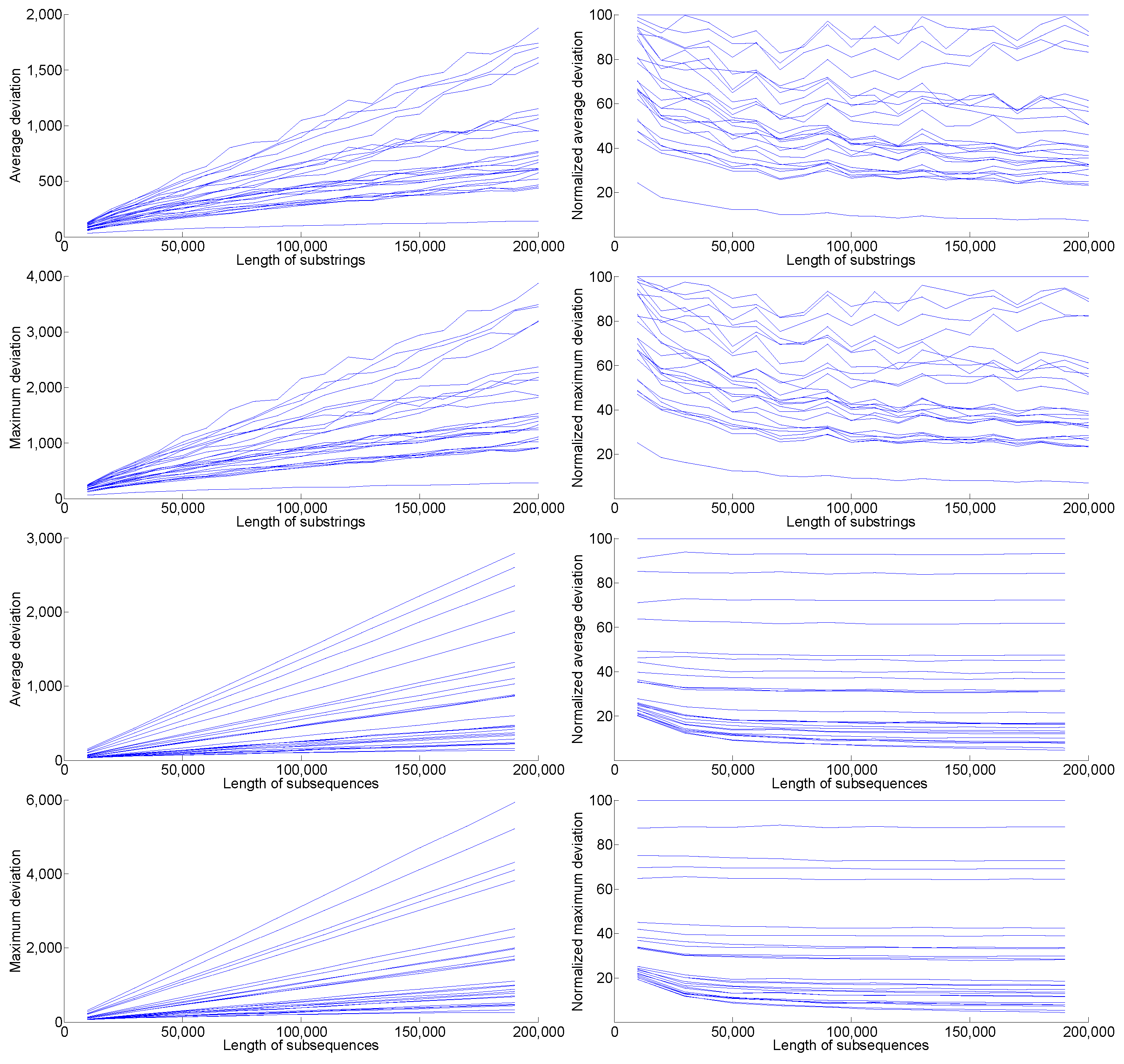

Table A1.
Normalized averages of 1000 trials
| Scientific Name | Common Name | Substrings | ||
| Random Sequence | Random | 12.8 | 12.8 | 100.0 |
| H. Sapiens | Human | 88.9 | 89.9 | 14.0 |
| H. Neanderthalensis | Neanderthal | 85.5 | 85.1 | 14.8 |
| G. Gorilla | Gorilla | 100.0 | 100.0 | 16.5 |
| P. Troglodytes | Chimp | 81.2 | 81.0 | 15.8 |
| C. Familiaris | Dog | 71.8 | 74.3 | 18.7 |
| G. Gallus | Chicken | 59.1 | 57.2 | 22.5 |
| C. Jacchus | Marmoset | 55.0 | 55.8 | 24.7 |
| R. Norvegicus | Rat | 68.2 | 68.0 | 22.9 |
| M. Musculus | Mouse | 62.5 | 64.9 | 19.8 |
| O. Anatinus | Platypus | 41.2 | 41.7 | 27.1 |
| A. Carolinensis | Lizard | 31.6 | 32.3 | 39.8 |
| D. Rerio | Zebrafish | 59.6 | 58.5 | 25.6 |
| O. Latipes | Medaka fish | 46.6 | 47.5 | 34.7 |
| D. Melanogaster | Fruit fly | 49.1 | 49.3 | 31.1 |
| C. Intestinalis | Sea squirt | 32.8 | 32.2 | 32.0 |
| C. Elegans | Nematode | 51.6 | 52.4 | 22.7 |
| S. Cerevisiae | Yeast | 39.4 | 39.8 | 27.4 |
| C. Muridarum | Chlamydia | 29.7 | 29.3 | 27.9 |
| M.Tuberculosis | Tuberculosis | 33.8 | 34.0 | 23.2 |
| P. Gingivalis | Gingivalis | 50.0 | 48.1 | 18.5 |
| S. Thermophilus | Streptococcus | 37.2 | 36.5 | 22.6 |
| O. Sativa | Rice | 73.8 | 76.9 | 24.5 |
| Z. Mays | Corn | 76.1 | 80.3 | 18.9 |
| A. Thaliana | Cress | 44.8 | 44.4 | 27.8 |
| G. Max | Soybean | 52.2 | 53.0 | 22.7 |
| Maximum pre-normalized value: | 554.5 | 1100.8 | 21.9 | |
Table A2.
Coefficient of variation (CV) and quartile coefficient of variation (QCV) of the 1000 trials
Table A2.
Coefficient of variation (CV) and quartile coefficient of variation (QCV) of the 1000 trials
| Common Name | Substrings | |||||
| CV | QCV | |||||
| Random | 0.24 | 0.21 | 0.45 | 0.16 | 0.14 | 0.27 |
| Human | 0.43 | 0.42 | 0.71 | 0.29 | 0.28 | 0.33 |
| Neanderthal | 0.43 | 0.42 | 0.72 | 0.26 | 0.27 | 0.33 |
| Gorilla | 0.52 | 0.48 | 0.86 | 0.35 | 0.34 | 0.67 |
| Chimp | 0.43 | 0.43 | 0.78 | 0.27 | 0.28 | 0.33 |
| Dog | 0.43 | 0.41 | 0.60 | 0.28 | 0.26 | 0.50 |
| Chicken | 0.48 | 0.46 | 0.97 | 0.37 | 0.36 | 0.50 |
| Marmoset | 0.44 | 0.42 | 0.61 | 0.26 | 0.24 | 0.40 |
| Rat | 0.59 | 0.61 | 0.76 | 0.41 | 0.39 | 0.56 |
| Mouse | 0.33 | 0.36 | 0.57 | 0.23 | 0.26 | 0.25 |
| Platypus | 0.42 | 0.38 | 0.58 | 0.24 | 0.23 | 0.45 |
| Lizard | 0.33 | 0.32 | 0.51 | 0.23 | 0.22 | 0.38 |
| Zebrafish | 0.41 | 0.36 | 0.57 | 0.28 | 0.26 | 0.40 |
| Medaka fish | 0.42 | 0.37 | 0.54 | 0.26 | 0.25 | 0.43 |
| Fruit fly | 0.48 | 0.46 | 0.69 | 0.35 | 0.32 | 0.50 |
| Sea squirt | 0.34 | 0.31 | 0.59 | 0.21 | 0.20 | 0.38 |
| Nematode | 0.36 | 0.35 | 0.55 | 0.26 | 0.21 | 0.33 |
| Yeast | 0.33 | 0.30 | 0.40 | 0.18 | 0.20 | 0.27 |
| Chlamydia | 0.34 | 0.28 | 0.49 | 0.23 | 0.20 | 0.33 |
| Tuberculosis | 0.42 | 0.41 | 0.71 | 0.25 | 0.26 | 0.40 |
| Gingivalis | 0.46 | 0.45 | 0.58 | 0.30 | 0.28 | 0.43 |
| Streptococcus | 0.37 | 0.34 | 0.54 | 0.22 | 0.22 | 0.40 |
| Rice | 0.47 | 0.45 | 0.54 | 0.30 | 0.29 | 0.40 |
| Corn | 0.45 | 0.45 | 0.56 | 0.31 | 0.35 | 0.50 |
| Cress | 0.29 | 0.29 | 0.49 | 0.20 | 0.18 | 0.27 |
| Soybean | 0.34 | 0.33 | 0.48 | 0.19 | 0.21 | 0.33 |
Table A3.
The ratio computed for substrings of length
| Human | 17.3 | 15.0 | 12.6 | 13.2 | 15.6 | 10.5 | 13.1 | 11.4 | 14.3 | 12.2 |
| Gorilla | 12.7 | 20.1 | 15.2 | 12.0 | 11.8 | 13.5 | 13.0 | 11.2 | 10.6 | 10.9 |
| Mouse | 19.9 | 28.1 | 30.8 | 40.2 | 37.9 | 41.7 | 45.2 | 57.1 | 46.7 | 50.0 |
| Zebrafish | 28.2 | 24.9 | 27.7 | 32.7 | 31.7 | 28.6 | 32.8 | 37.0 | 26.6 | 40.8 |
| Tuberculosis | 44.6 | 64.8 | 66.5 | 84.6 | 88.1 | 96.5 | 105.1 | 116.3 | 122.5 | 144.9 |
| Random Sequence | 126.7 | 164.3 | 205.7 | 260.2 | 280.7 | 304.7 | 325.1 | 336.0 | 351.2 | 397.0 |
| 1 | For the notion of negentropy see Section 3.5. |
| 2 | |
| 3 | Often when a mathematician is asked to explain why certain bizarre mathematical fact may be true, the answer in mathematical jargon is “That’s life!" |
| 4 | This term refers to the observation that some organisms have the potential to adapt to changing environments very rapidly and comprehensively than others. |
| 5 | Genetic recombination (reshuffling) is the exchange of genetic material between different organisms which results in fabrication of offspring that combine traits different from those found in the parents. |
| 6 | Note that this layout does not contradict the findings about the hypothetical common ancestor of all known living things, known as the Last Universal Common Ancestor (LUCA); it is known that LUCA was not the first form of life, and life forms had existed long before it, probably a billion of years prior to LUCA [33] |
References
- Agarwal, P.; Aronov, B.; Sharir, M. Line transversals of balls and smallest enclosing cylinders in three dimensions. Discrete & Computational Geometry 1999, 21(3), 373–388. [Google Scholar] [CrossRef]
- Apostolico, A.; Giancarlo, R. Sequence alignment in molecular biology. Journal of Computational Biology 1998, 5(2), 173–196. [Google Scholar] [CrossRef] [PubMed]
- Apostolico, A.; Cunial, F. Probing the randomness of proteins by their subsequence composition. Proc. Data Compression Conference DCC ’09, NW Washington, DC, United States, 2009, 173–182.
- Apostolico, A.; Cunial, F. The subsequence composition of polypeptides. Journal of Computational Biology 2010, 17(8), 1–39. [Google Scholar] [CrossRef] [PubMed]
- Apostolico, A.; Z. Galil, Z. (Eds.) Pattern Matching Algorithms; Oxford University Press: New York, USA, 1997. [Google Scholar]
- Brimkov, B. Geometric approach to string analysis for biosequence classification. J. Integr. Bioinform. 2014, 11(3). [Google Scholar] [CrossRef]
- Brimkov, B.; Brimkov, V.E. Brimkov, B., Brimkov, V.E. Geometric approach to string analysis: deviation from linearity and its use for biosequence classification. arXiv:1308.2885, https://arxiv.org/pdf/1308.2885 2013.
- Brimkov, B.; Brimkov, V.E. Geometric Approach to Biosequence Analysis. Proc. 8th International Conference on Practical Applications of Computational Biology and Bioinformatics, Salamanca, Spain, 2014, 97–104.
- Broox, F.P., Jr. Three great challenges for half-century-old computer science. J. ACM 2003, 50, 25–26. [Google Scholar]
- Behe, M.J. Darwin’s Black Box: The Biochemical Challenge to Evolution. In Touchstone book, 2 ed.; Free Press: United States, 2006. [Google Scholar]
- Cairns-Smith, A.G. Seven Clues to the Origin of Life: A Scientific Detective Story; Cambridge University Press, 1990. [Google Scholar]
- Chan, T. Approximating the diameter, width, smallest enclosing cylinder, and minimum-width annulus. Proc. 16th Annual Symposium on Computational Geometry, Clear Water Bay, Kowloon, Hong Kong, 2000, 300–309.
- Cormen, Th.H.; Leiserson, Ch.E.; Rivest, R.L.; Stain, C. Introduction to Algorithms; MIT Press & McGraw Hill: Cambridge, Mass., 2001. [Google Scholar]
- Crochemore, M.; Rytter, W. Text Algorithms; Oxford University Press, 1994. [Google Scholar]
- Darwin, Ch.M.A. On the Origin of Species by Means of Natural Selection, or the Preservation of Favoured Races in the Struggle for Life; New York, D. Appleton & Co., 1859. [Google Scholar]
- Davies, P. The Fifth Miracle: The Search for The Origin and Meaning of Life; Simon & Schuster, 2000. [Google Scholar]
- Deamer, D. First Life: Discovering the Connections between Stars, Cells, and How Life Began; University of California Press, 2012. [Google Scholar]
- Devillers, O.; Preparata, F. Evaluating the cylindricity of a nominally cylindrical point set. Proc. SODA, San Francisco, California, USA, 2000, SIAM publisher, 518–527.
- Dyson, F. Origins of Life; Cambridge University Press, 1999. [Google Scholar]
- ErdPos, P.; Gyori, E.; Simonovits, M. How many edges should be deleted to make a triangle-free graph bipartite? In Sets, Graphs and Numbers; Budapest, Hungary, 1991; Colloq. Math. Soc. János Bolyai, 60, 239-263, North-Holland, Amsterdam, 1992. [Google Scholar]
- Fry, I. Emergence of Life on Earth: A Historical and Scientific Overview; Rutgers University Press, 2000. [Google Scholar]
- Garey, M.; Johnson, D. Computers and Intractability; W.H. Freeman & Company: San Francisco, 1979. [Google Scholar]
- Gates, M. A simple way to look at DNA. Journal of Theoretical Biology 1986, 119(3), 319–328. [Google Scholar] [CrossRef] [PubMed]
- Haldane, J.B.S. The Origin of Life. The Rationalist Annual 1929, 148, 3–10. [Google Scholar]
- Hazen, R. Genesis: The Scientific Quest for Life’s Origin; National Academies Press, 2005. [Google Scholar]
- Kell, D.B. Scientific discovery as a combinatorial optimization problem: How best to navigate the landscape of possible experiments? BioEssays 2012, 34(3), 163–251. [Google Scholar] [CrossRef] [PubMed]
- Klette, R.; Rosenfeld, A. Digital Geometry – Geometric Methods for Digital Picture Analysis; Morgan Kaufmann: San Francisco, 2004. [Google Scholar]
- Lane, N. The Vital Question: Energy, Evolution, and the Origins of Complex Life; W. W. Norton and Company, Inc., 2015. [Google Scholar]
- Leong, P.M.; Morgenthaler, S. Random walk and gap plots of DNA sequences. Comput. Appl. Biosci. 1995, 11(5), 503–507. [Google Scholar] [CrossRef] [PubMed]
- Lovász, L. Large Networks and Graph Limits, American Mathematical Society, Colloquium Publications, Vol. 60, 2012, https://lovasz.web.elte.hu//bookxx/hombook-almost.final.pdf.
- Luisi, P.L. The Emergence of Life: From Chemical Origins to Synthetic Biology; Cambridge University Press, 2010. [Google Scholar]
- Monod, J. Chance and Necessity; Collins: London, 1972. [Google Scholar]
- Moody, E.; Álvarez-Carretero, S.; Mahendrarajah, T. The nature of the last universal common ancestor and its impact on the early Earth system. Nature Ecology and Evolution 2024, 8(9), 1654–1666. [Google Scholar] [CrossRef] [PubMed]
- Morowitz, H.J. Beginnings of Cellular Life: Metabolism Recapitulates Biogenesis; Yale University Press, 2004. [Google Scholar]
- Nevil-Manning, C.; Witten, I. Protein is incompressible. Proc. Conf. Data Compression, Snowbird, Utah, USA, 1999, p. 257.
- Oparin, A.I. Vozniknovenie zhizni na zemle (The Origin of Life on Earth), Moscow, Izd. Akad. Nauk SSSR, 1936.
- Pigliucci, M. Design Yes, Intelligent No. A Critique of Intelligent Design Theory and Neo-Creationism, 2000, Internet Infidels, http://www.infidels.org/library/modern/features/2000/pigliucci1.html.
- Salzburger, W.; Steinke, D.; Braasch, I.; Meyer, A. Genome desertification in eutherians: can gene deserts explain the uneven distribution of genes in placental mammalian genomes? J. Mol. Evol. 2009, 69(3), 207–216. [Google Scholar] [CrossRef] [PubMed]
- Sankoff, D.; Kruskal, J.B. (Eds.) Time Warps, String Edits, and Macromolecules: The Theory and Practice of Sequence Computation; Addison-Wesley: Reading, MA, 1983. [Google Scholar]
- Schopf, J.W. (Ed.) Life’s Origin: The Beginnings of Biological Evolution; University of California Press, 2002. [Google Scholar]
- Schwartz, R.; King, J. Sequences of hydrophobic and hydrophilic runs and alternations in proteins of known structure. Protein Sci. 2006, 15, 102–112. [Google Scholar] [CrossRef] [PubMed]
- Pande, V.; Grosberg, A.; Tanaka, T. Nonrandomness in protein sequences: evidence for a physically driven stage of evolution. Proc. Natl. Acad. Sci. USA 1994, 91, 12972–12975. [Google Scholar] [CrossRef] [PubMed]
- Pross, A. What is Life?: How Chemistry Becomes Biology; Oxford University Press, 2012. [Google Scholar]
- Rasmussen, S.; Bedau, M.A.; Chen, L.; Deamer, D.; Krakauer, D.C.; Packard, N.H.; Stadler, P.F. (Eds.) Protocells: Bridging Nonliving and Living Matter; The MIT Press, 2008. [Google Scholar]
- Rauchfuss, H. Chemical Evolution and the Origin of Life; Springer Verlag, 2008. [Google Scholar]
- Russell, M. (Ed.) Abiogenesis: How Life Began. The Origins and Search for Life; Cosmology Science Publishers, 2011. [Google Scholar]
- Schrodinger, E. What is Life? Cambridge University Press, 1944. [Google Scholar]
- Schulze-Makuch, D.; Irwin, L.N. Life in the Universe: Expectations and Constraints (Advances in Astrobiology and Biogeophysics); Springer, 2008. [Google Scholar]
- Smith, E.; Morowitz, H. The Origin and Nature of Life on Earth: The Emergence of the Fourth Geosphere; Cambridge University Press, 2016. [Google Scholar]
- Smith, J.M.; Szathmáry, E. The Origins of Life: From the Birth of Life to the Origin of Language; Oxford University Press, 2000. [Google Scholar]
- Sullivan III, W.T.; Baross, J.B. (Eds.) Planets and Life: The Emerging Science of Astrobiology; Cambridge University Press, 2007. [Google Scholar]
- Than, K. Why scientists dismiss ’intelligent design’, LiveScience, NBC News. 2005. [Google Scholar]
- Vanchurin, V.; Wolf, Y.I.; Koonin, E.V.; Katsnelson, M.I. Thermodynamics of evolution and the origin of life, https://www.pnas.org/doi/epub/10.1073/pnas.2120042119, Proc. Natl. Acad. Sci. USA, 2022.
- Waterman, M.S. Introduction to Computational Biology. Maps, Sequences and Genomes; Chapman Hall, 1995. [Google Scholar]
- Weiss, O.; Jiménez-Montañgo, M.; Herzel, H. Information content of protein sequences. J. Theoret. Biology 2000, 206, 379–386. [Google Scholar] [CrossRef] [PubMed]
- White, S.; Jacobs, R. Statistical distribution of hydrophobic residues along the length of protein chains. Biophys. J. 1990, 57, 911–921. [Google Scholar] [CrossRef] [PubMed]
- Wills, Ch.; Bada, J. The Spark Of Life: Darwin And The Primeval Soup; Oxford University Press: Oxford New York, 2001. [Google Scholar]
- Yoder, N. PeakFinder (update 2011, File ID: #25500), Matlab Central, http://www.mathworks.com/matlabcentral/fileexchange/25500-peakfinder.
- Abiogenesis, https://en.wikipedia.org/wiki/Abiogenesis.
- Zubay, G. Origins of Life: On Earth and in the Cosmos, 2nd Ed. ed; Academic Press, 2000. [Google Scholar]
Figure 1.
Left: Regular triangular helix (regular skew-apeirogon). Right: Irregular triangular helix (irregular skew-apeirogon).
Figure 1.
Left: Regular triangular helix (regular skew-apeirogon). Right: Irregular triangular helix (irregular skew-apeirogon).
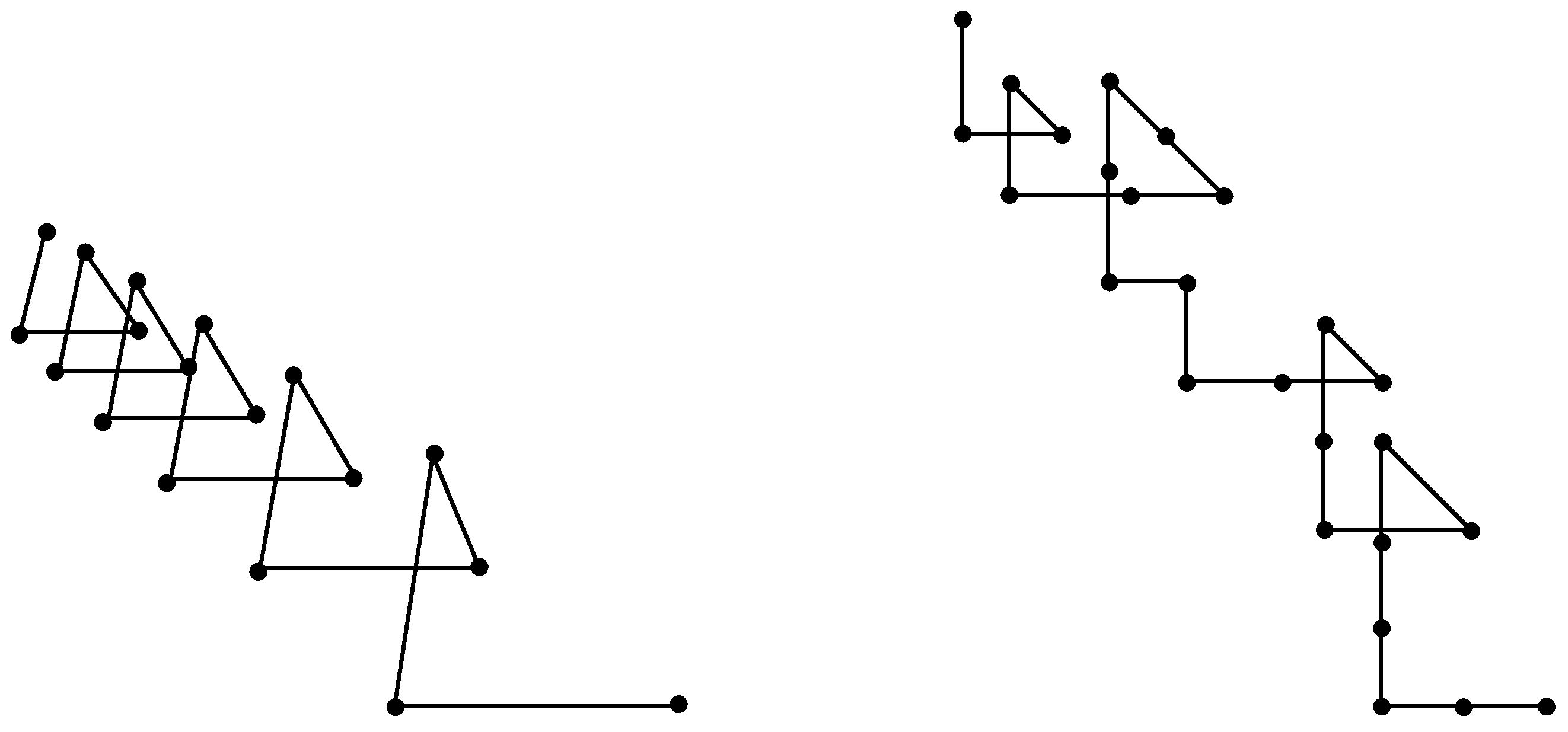
Figure 2.
Illustration to the structure of the global life network.
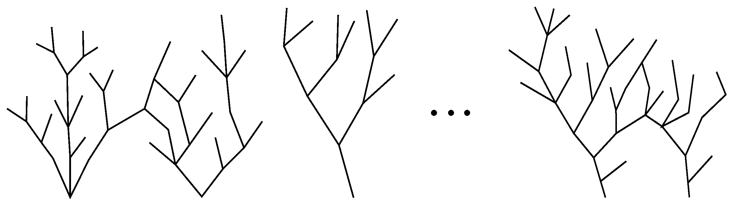
Disclaimer/Publisher’s Note: The statements, opinions and data contained in all publications are solely those of the individual author(s) and contributor(s) and not of MDPI and/or the editor(s). MDPI and/or the editor(s) disclaim responsibility for any injury to people or property resulting from any ideas, methods, instructions or products referred to in the content. |
© 2025 by the authors. Licensee MDPI, Basel, Switzerland. This article is an open access article distributed under the terms and conditions of the Creative Commons Attribution (CC BY) license (http://creativecommons.org/licenses/by/4.0/).
Copyright: This open access article is published under a Creative Commons CC BY 4.0 license, which permit the free download, distribution, and reuse, provided that the author and preprint are cited in any reuse.


