1. Introduction
High-resolution land surface temperature (LST) products are required in several applied domains. In precision agriculture, field-scale thermal patterns support irrigation timing, detection of crop water stress, and yield-related diagnostics. These tasks need spatial detail below the scale of typical numerical weather prediction (NWP) grids. [
1,
2,
3] Local decision workflows also benefit from combining satellite information with dense, near-surface meteorological predictions. This includes fusion of global forecasts with station data and land reanalysis to improve actionable temperature estimates for farms. [
4,
5,
6] Beyond agriculture, high-resolution LST is used to quantify urban heat exposure, to parameterize energy-balance models, and to characterize surface extremes driving hydrological hazards. [
7] These application demands motivate methods that provide LST at fine spatial resolution with continuous temporal coverage.
LST is an essential climate variable. It links the surface energy balance with boundary-layer processes. It is therefore used in climate monitoring, evapotranspiration modeling, and drought or heat-wave assessment. [
8] However, high spatial resolution and high temporal frequency are rarely available in the same product. NWP and reanalysis data such as ERA5 provide hourly continuity, but their spatial resolution remains coarse for heterogeneous landscapes. [
9] Land-focused reanalyses such as ERA5-Land improve spatial detail but still do not resolve field-scale thermal contrasts. [
10] In contrast, Landsat thermal infrared (TIR) observations provide LST close to 100 m. Their revisit interval is about 8 days and observations are clear-sky only. [
11]
Cloud contamination is the main limit of TIR-based LST. Globally, clouds obscure land surfaces for most overpasses. As a result, LST fields derived from optical TIR sensors contain large spatial and temporal gaps. [
12] Accurate masking of clouds and cloud shadows is therefore a key preprocessing step. The Fmask family of algorithms is a standard baseline for Landsat cloud detection. [
13] In ALIANCE first-year work we developed operational workflows for cloud-robust land monitoring and local temperature forecasting. [
4,
14] The present study extends these results. It adds improved cloud masking for the Landsat thermal band and uses the resulting clear-sky patches for supervised fusion with NWP data.
Several approaches target all-weather or gap-free LST. A common direction is multi-sensor fusion of TIR with passive microwave (PMW) observations, because PMW penetrates clouds but has coarse resolution. Random-forest fusion of MODIS with PMW brightness temperatures has provided daily all-weather LST and reduced cloud-induced gaps. [
15,
16] Other studies apply physically consistent PMW retrieval under clouds. [
20] An alternative route merges TIR with model temperatures using radiative transfer or statistical decomposition, thus exploiting temporal continuity of NWP or reanalysis fields. [
17]
Purely data-driven gap filling has also progressed. MDINEOF integrates radiative flux drivers into empirical orthogonal reconstruction and improves cloudy-sky LST without PMW data. [
8] GraphProp models pixels as graph nodes and propagates clear-sky values across spectral-spatial neighborhoods, achieving low error even under extreme cloud cover. [
18] Physically based optical methods further exploit solar–cloud–satellite geometry to estimate sub-cloud LST from TIR scenes. [
19] These approaches provide gap reduction but do not directly address superresolution from coarse model grids to Landsat scale.
Superresolution and spatiotemporal fusion methods aim to transfer temporal frequency from coarse sensors or models to fine TIR grids. Early work evaluated thermal disaggregation of MODIS toward Landsat-like resolution. [
21] Recent fusion frameworks combine Landsat and MODIS to reconstruct high-resolution LST series. [
22,
23] Spatial downscaling components are often embedded through geographically weighted regression or machine-learning predictors. [
24,
25] Hybrid pipelines that couple spatial downscaling with spatiotemporal fusion show improved robustness across landscapes and seasons. [
26] Continental products at 100 m and daily or hourly frequency have been demonstrated using unbiased fusion or multistage assimilation, but they still require sufficient clear-sky satellite inputs and usually depend on multi-sensor TIR availability. [
27,
28]
In this paper we propose a two-stage fusion strategy to derive 100 m LST from coarse NWP temperature fields and sporadic Landsat observations. The method follows the physical complementarity of sources. ICON-EU provides hourly surface temperature proxies at ~7 km. Landsat provides fine-scale TIR structure for clear-sky moments. A convolutional network with U-Net topology learns the mapping from the coarse NWP field and recent Landsat context to the current Landsat-scale LST. [
29]
Research objectives.
This study aims to:
Train a deep fusion model that super-resolves hourly ICON-EU surface temperatures to 100 m using Landsat context.
Quantify accuracy and temporal consistency of the fused LST against Landsat clear-sky observations.
Demonstrate domain relevance for agricultural and environmental applications requiring all-weather, field-scale thermal dynamics.
2. Materials and Methods
2.1. Study Area
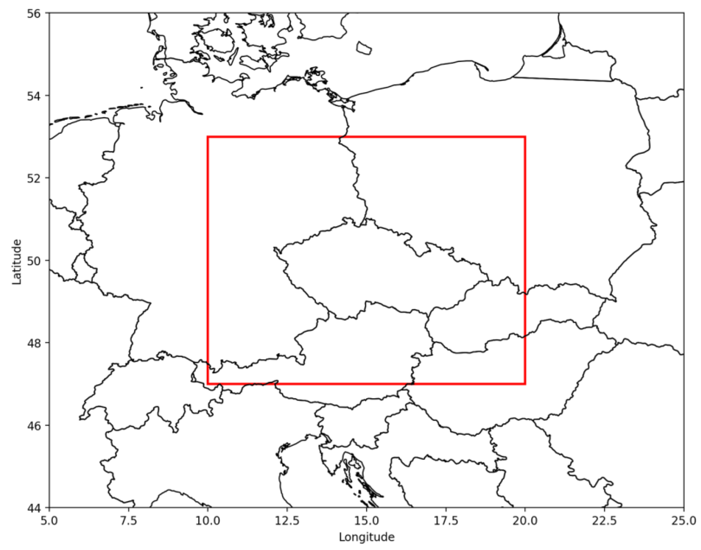
The study area covers central Europe, from 47° N to 53° N and from 10° E to 20° E. The region includes Central European lowlands, hilly terrain, and Alpine foreland. Land cover is dominated by arable land, grassland, forest, and urban areas. This heterogeneity is suitable for evaluating superresolution of land surface temperature (LST) across a range of surface types and roughness conditions.
The analysis domain is discretized into fixed tiles of 256 × 256 Landsat pixels (about 25 × 25 km). All training and validation samples are subwindows of these tiles. Only samples with sufficient valid clear-sky LST targets are retained for model training and evaluation.
Figure 1.
Region of interest.
Figure 1.
Region of interest.
2.2. Data
2.2.1. Landsat 8/9
Landsat 8 and Landsat 9 Level-2 Tier 1 Surface Reflectance products are used as the primary high-resolution data source. Products are accessed via Google Earth Engine using the LANDSAT/LC08/C02/T1_L2 and LANDSAT/LC09/C02/T1_L2 collections. These datasets provide atmospherically corrected surface reflectance in the visible to shortwave infrared bands and a thermal infrared (TIR) band processed to orthorectified surface temperature. [
11]
Cloud-, cloud-shadow-, and snow-contaminated pixels are excluded using the QA_PIXEL band and the associated CFMask/Fmask-derived bit flags provided with the Landsat Collection 2 Level-2 product. [
13] In this study, masking is treated strictly as a preprocessing step to define reliable clear-sky reference pixels for training and validation; we do not introduce, modify, or evaluate a new cloud-detection procedure or a dedicated thermal-band cloud mask. Where needed to minimize residual contamination (e.g., thin cirrus or mixed cloud–land edges), the clear-sky selection may be conservatively tightened using established thermal-quality screening rules reported in prior work, applied as a fixed filter rather than as a methodological contribution. [
14]
LST is expressed in degrees Celsius and resampled to a common grid of 0.001° (≈100 m) for all scenes. Only pixels flagged as clear by QA_PIXEL (and passing the conservative thermal-quality screening, where applied) are retained as targets for model training and validation.
Landsat 8 and 9 jointly provide a nominal revisit of approximately 8 days at the equator, with shorter effective intervals at the higher latitudes of the study area. Over central Europe, overpass time is around 09:30–10:30 UTC, which defines the local time window for NWP–satellite matching.
2.2.2. ICON-EU Surface Temperature
Among the operational numerical weather prediction (NWP) models, ICON (ICOsahedral Nonhydrostatic) provides a regional European configuration (ICON-EU) with a spatial resolution of about 0.06° (≈7 km) and high update frequency. ICON-EU forecasts are available via the DWD Open Data portal and through the Open-Meteo Historical Forecast API. [
12,
13,
14,
15]
The variable soil_temperature_0cm from ICON-EU is used as the coarse-resolution temperature input. This variable approximates the temperature at the land–atmosphere interface and is therefore the closest model analogue to satellite-derived LST. For each Landsat overpass, the forecast with 0 h lead time closest in time to the acquisition is selected. This minimizes forecast error and aligns the model state with the observation time.
ICON-EU outputs are provided at hourly resolution by temporal interpolation of the 3-hourly native forecast cycles. The corresponding model grid is reprojected and resampled to the Landsat grid using bilinear interpolation. The resulting ICON-EU field at 100 m resolution is used as input to the fusion model and to the baseline comparison.
2.2.3. Temporal Matching and Feature Construction
For each Landsat tile and date, a training or validation sample is constructed if the target Landsat scene has sufficient clear-sky coverage in the thermal band after standard QA_PIXEL-based clear-sky screening (Fmask/CFMask flags), used solely to define training/validation reference pixels, and the corresponding ICON-EU forecast at 0 h lead time is available within ±30 min of the Landsat overpass.
Each sample consists of: the thermal Landsat target, a sequence of up to five most recent Landsat acquisitions over the tile (all surface-reflectance bands and the thermal band), andthe temporally matched ICON-EU soil_temperature_0cm field, resampled to the Landsat grid.
The data are aligned to the common model grid.
2.3. Model Architecture
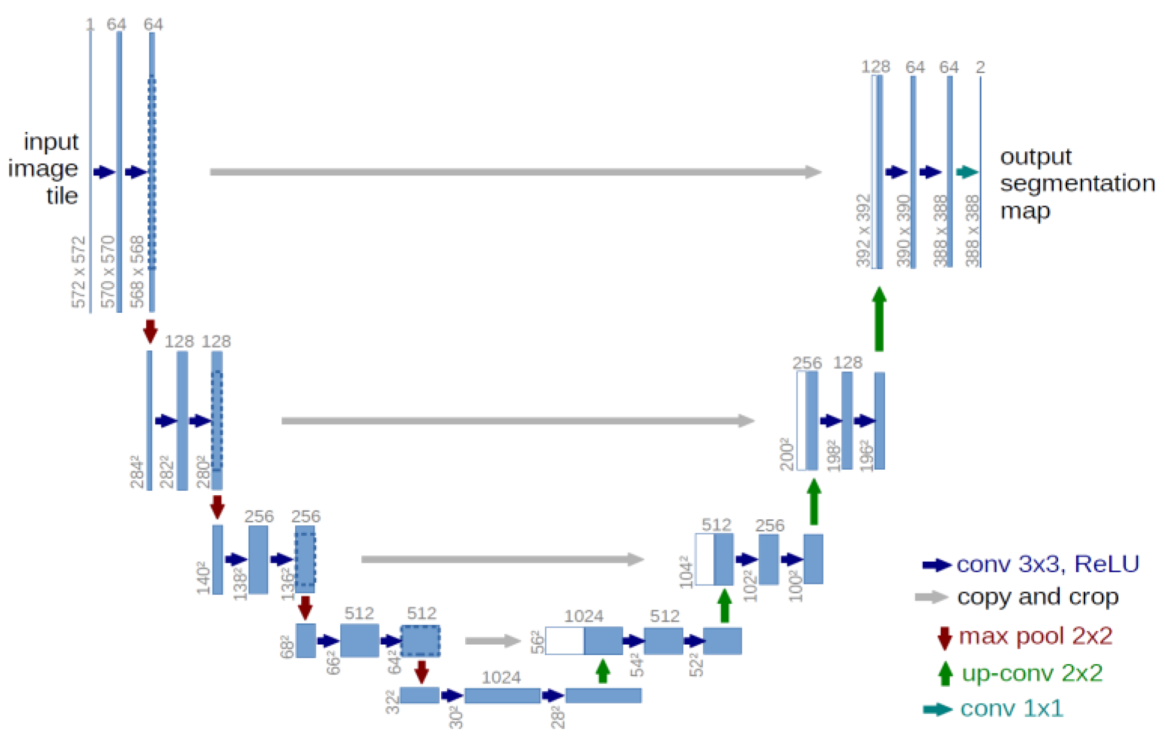
The baseline model is a convolutional encoder–decoder network based on the U-Net architecture. [
16,
29] U-Net is widely used in remote sensing for dense prediction tasks due to its symmetric contracting and expanding paths and skip connections, which preserve fine spatial detail.
The network operates on 256 × 256 pixel patches. The Landsat sequence is flattened in the channel dimension and concatenated with the upscaled ICON-EU temperature field, producing a multi-channel input tensor. This allows early layers to learn joint spectral–temporal features from the satellite data while conditioning on the coarse-scale temperature field from ICON-EU.
Figure 2.
U-Net architecture [
29].
Figure 2.
U-Net architecture [
29].
The encoder consists of successive convolutional blocks with 3 × 3 kernels, each followed by non-linear activation and downsampling via max-pooling. The decoder applies transpose convolutions (or bilinear upsampling with convolutions) to restore spatial resolution, concatenating encoder feature maps via skip connections at each level. The final layer is a 1 × 1 convolution that outputs a single LST channel at Landsat resolution.
Training uses mean absolute error (MAE) between predicted and reference Landsat LST as loss function. MAE is preferred over mean squared error because it is less sensitive to outliers and its units are directly interpretable as degrees Celsius.
Optimization is performed with mini-batch stochastic gradient descent using a batch size of 16. Weight updates use the Adam optimizer with standard parameters. Training continues until convergence of the validation loss, monitored over the independent validation year.
2.4. Experimental Design and Validation
2.4.1. Train–Validation Split
The training set consists of all valid tiles over the study area for the full calendar year 2023. The validation set uses the full year 2024 and is spatially overlapping but temporally disjoint from the training period. This split tests generalization across interannual variability in temperature and cloudiness.
2.4.2. Baselines
Two ICON-EU baselines are defined for comparison:
ICON-EU nearest: ICON-EU soil_temperature_0cm field resampled to the Landsat grid using nearest-neighbor interpolation;
ICON-EU linear: ICON-EU soil_temperature_0cm field resampled using bilinear interpolation.
Both baselines are evaluated against Landsat LST using the same metrics as the U-Net model. This isolates the added value of the fusion network relative to simple spatial interpolation of the NWP field.
2.4.3. Accuracy Metrics
Model and baseline performance are evaluated using mean absolute error (MAE) and root mean square error (RMSE) computed over all valid pixels in the validation set.
All metrics are computed on the original LST scale without additional detrending or bias correction. Separate aggregations by season and land-cover class can be derived but are not required for the core validation protocol.
3. Results
3.1. Quantitative Performance Relative to ICON-EU Baselines
The U-Net fusion baseline improves Landsat-scale LST reconstruction relative to direct ICON-EU upscaling. On the independent validation year (2024), the U-Net reaches MAE = 2.55 °C and RMSE = 3.50 °C. The linearly interpolated ICON-EU field reaches MAE = 3.24 °C and RMSE = 4.48 °C. Nearest-neighbor ICON-EU gives similar error (MAE = 3.26 °C; RMSE = 4.50 °C). The fusion therefore reduces MAE by 0.69 °C and RMSE by 0.98 °C compared with the linear baseline.
Table 1 reports the aggregate validation accuracy over all clear-sky pixels. It provides the primary comparison between the fusion model and the two ICON-EU interpolation baselines.
The gain indicates that the model learns a stable mapping between coarse NWP temperature structure and fine-scale Landsat thermal patterns. It reduces the smoothing error inherent to the NWP grid and corrects part of the systematic warm-season bias.
Seasonal stratification tests if the mapping remains stable across solar forcing regimes and if residual biases are concentrated in summer or winter.
Table 2.
Seasonal performance (validation year).
Table 2.
Seasonal performance (validation year).
| Season |
ICON-EU linear MAE (°C) |
U-Net MAE (°C) |
ICON-EU linear RMSE (°C) |
U-Net RMSE (°C) |
| DJF |
2.16 |
2.36 |
3.22 |
3.12 |
| MAM |
3.49 |
2.69 |
4.66 |
3.62 |
| JJA |
4.01 |
2.77 |
5.37 |
3.88 |
| SON |
2.51 |
2.23 |
3.47 |
3.03 |
Land-cover stratification evaluates whether the model correctly handles surfaces with different emissivity, heat capacity, and sub-grid heterogeneity such as cropland, forest, and urban areas.
Table 3.
Performance by land-cover (using ESA WorldCover v200) class (validation year).
Table 3.
Performance by land-cover (using ESA WorldCover v200) class (validation year).
| Class |
N pixels |
ICON-EU linear MAE (°C) |
U-Net MAE (°C) |
ICON-EU linear RMSE (°C) |
U-Net RMSE (°C) |
| Tree cover |
46316857 |
2.37 |
2.29 |
3.31 |
3.13 |
| Grassland |
19331399 |
3.62 |
2.64 |
4.74 |
3.61 |
| Cropland |
34294237 |
3.98 |
2.78 |
5.35 |
3.81 |
| Built-up |
4279537 |
4.76 |
2.85 |
6.01 |
3.84 |
| Snow and ice |
25935 |
9.11 |
7.54 |
10.15 |
8.52 |
| Water bodies |
1177626 |
3.23 |
2.65 |
4.25 |
3.69 |
Error by temperature regime identifies whether improvements persist at cold and hot extremes. This is important for heat-stress and drought monitoring use cases.
Table 4.
Error by temperature regime (validation year).
Table 4.
Error by temperature regime (validation year).
| LST quantile |
ICON-EU linear MAE (°C) |
U-Net MAE (°C) |
| 0–25% |
2.23 |
2.48 |
| 25–50% |
2.34 |
2.35 |
| 50–75% |
2.83 |
2.22 |
| 75–100% |
5.56 |
3.13 |
The robustness of reconstruction under limited clear-sky availability is assessed by stratifying errors against the cloud fraction in each Landsat tile.
Table 5.
Error versus cloud fraction in the Landsat tile (evaluation on valid clear-sky pixels).
Table 5.
Error versus cloud fraction in the Landsat tile (evaluation on valid clear-sky pixels).
| Cloud fraction bin |
N scenes |
ICON-EU linear MAE (°C) |
U-Net MAE (°C) |
| 0–20% |
21 |
3.72 |
2.38 |
| 20–40% |
235 |
3.73 |
2.49 |
| 40–60% |
504 |
3.28 |
2.50 |
| 60–80% |
614 |
3.17 |
2.55 |
| 80–100% |
244 |
2.79 |
2.69 |
3.2. Random Spatial Reconstruction Examples
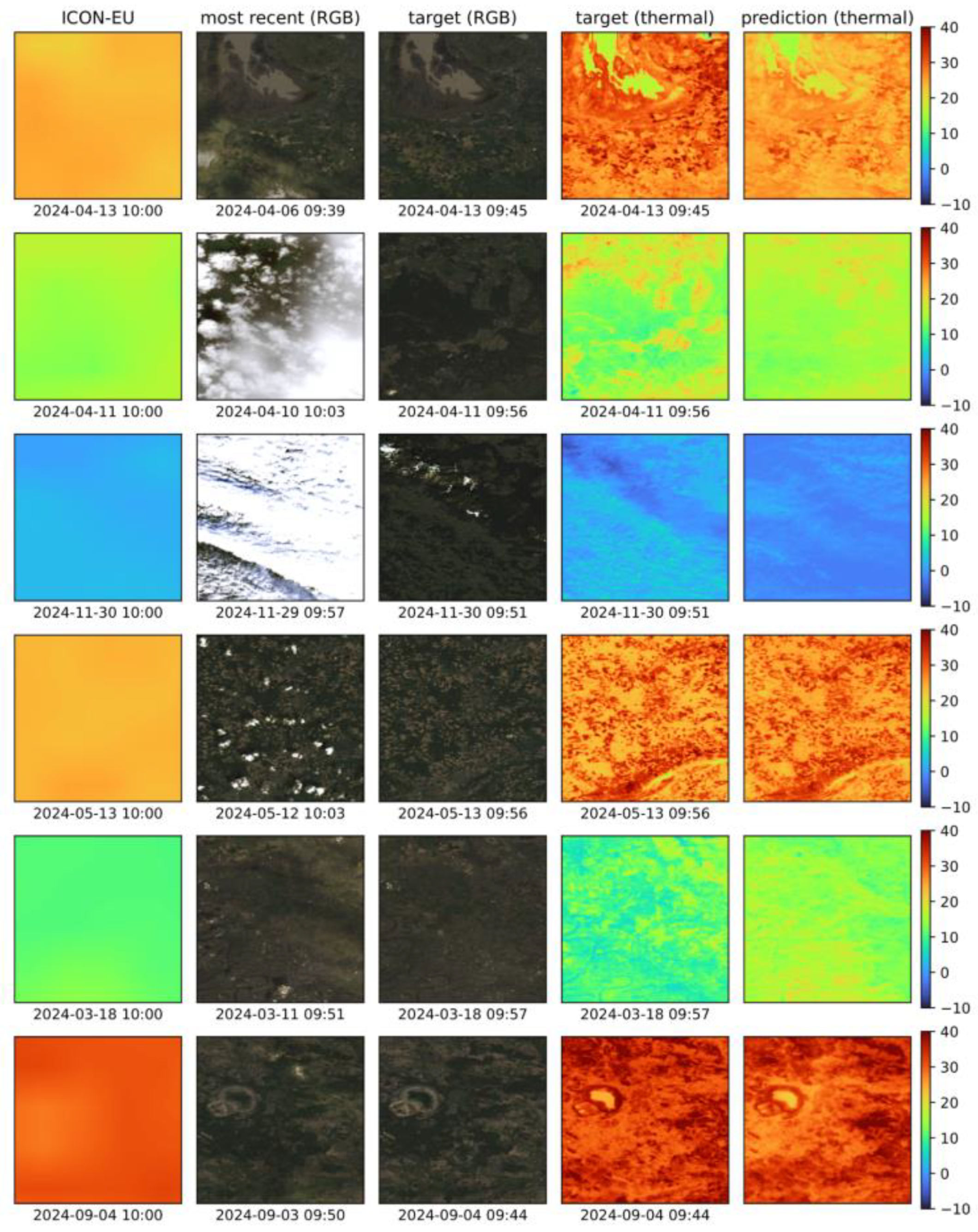
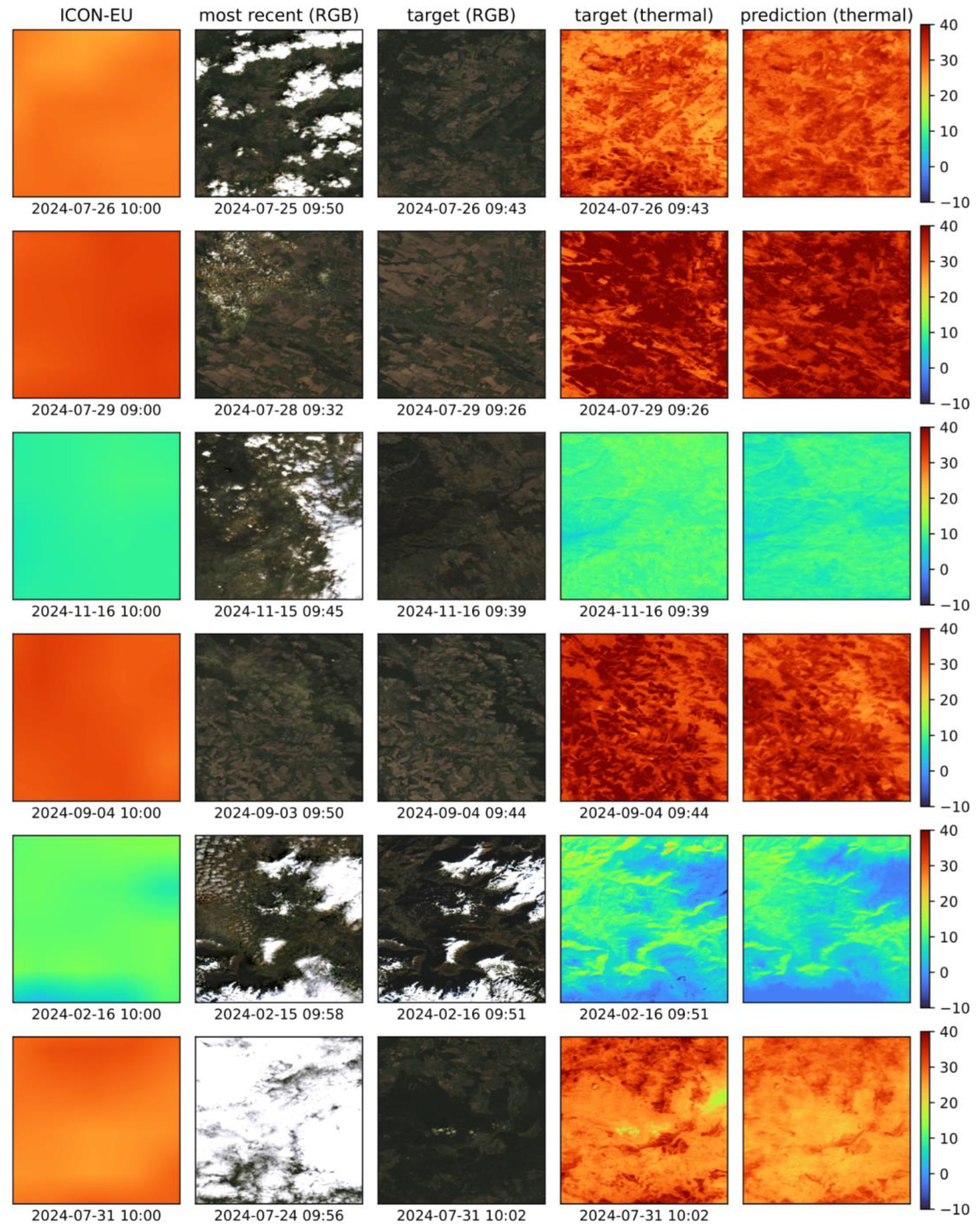
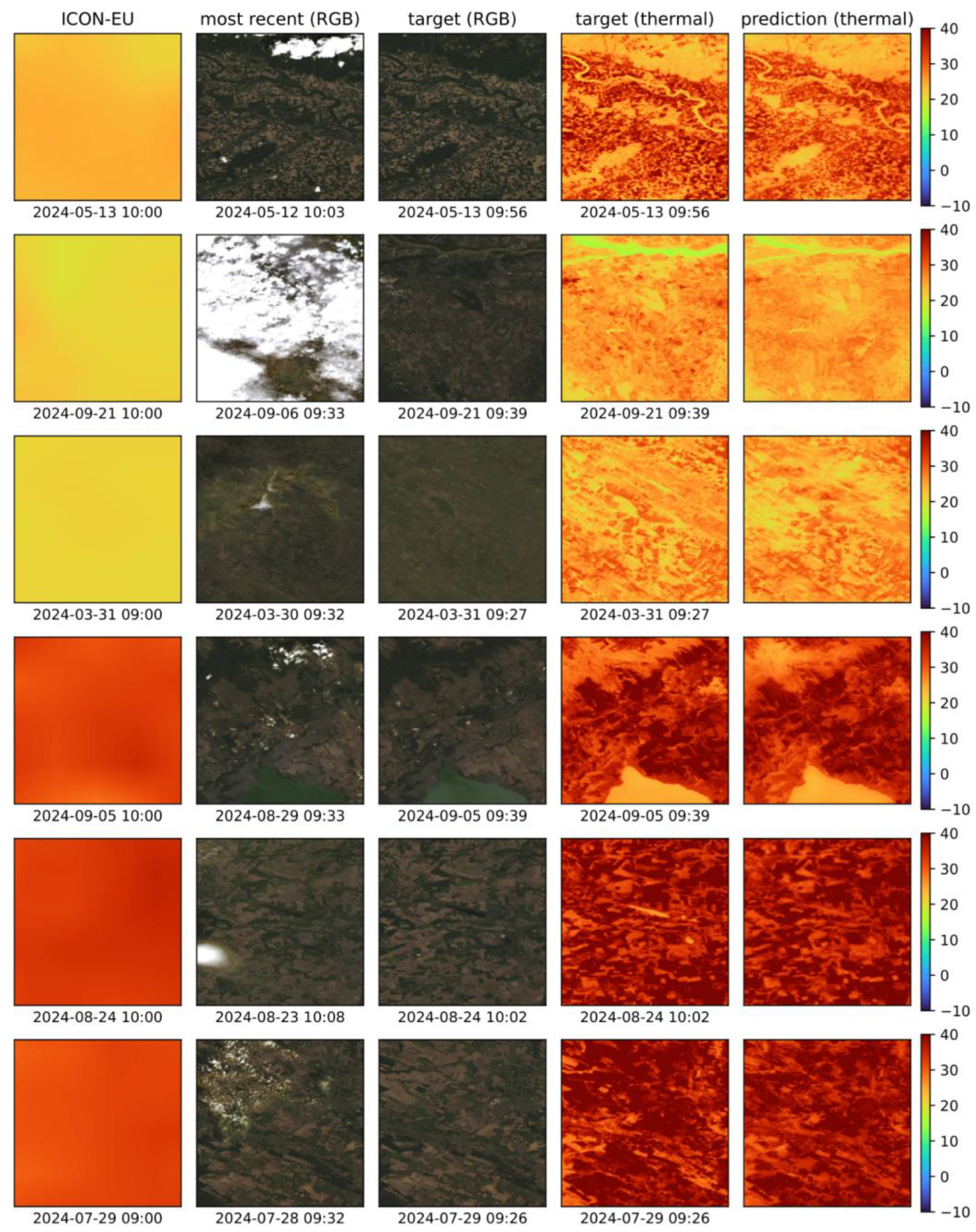
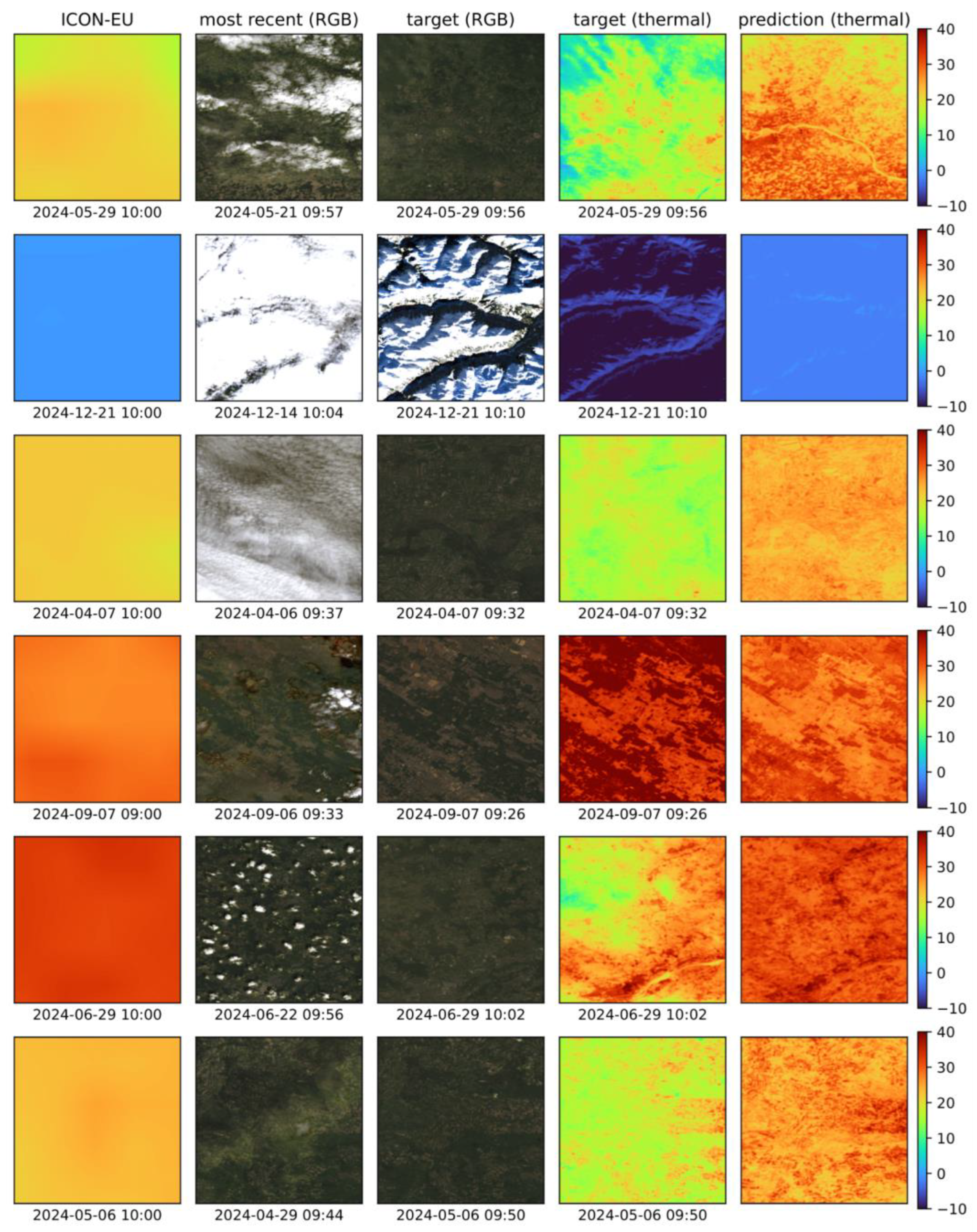
Figure 3 and
Figure 4 show randomly selected validation samples. Each row corresponds to one sample. Columns are: (i) ICON-EU soil_temperature_0cm resampled to Landsat grid, (ii) most recent Landsat RGB image before the target date, (iii) target RGB Landsat image (only shown for reference, not actually used in our method), (iv) target clear-sky Landsat thermal LST, and (v) U-Net predicted LST. The thermal color scale spans −10 to 40 °C.
Description: The examples cover spring, summer, autumn, and winter conditions. Several rows include partial cloud in the most recent RGB input. The U-Net output reproduces field-scale and forest-edge thermal texture visible in the target thermal panel. ICON-EU fields are spatially smooth. The fused product retains ICON-EU large-scale temperature level while adding fine gradients aligned with land-cover structure.
Description: The set emphasizes warm-season surfaces and mixed cloud histories. In rows with strong insolation and high target LST, ICON-EU under-represents local maxima. The U-Net reconstructs sharper thermal edges, including within agricultural mosaics and along linear landscape features. In colder cases, the model reproduces broad cooling patterns without introducing artificial warm spots.
3.3. Best-Case Improvements
Figure 5 presents samples with the largest MAE improvement over ICON-EU. These are typically warm-season scenes with high surface heterogeneity.
Description: Hot surfaces approaching 35–40 °C are systematically underpredicted by ICON-EU. The U-Net corrects this bias and restores locally amplified heating patterns. The improvement is visible as higher thermal contrast and better delineation of hot pixels that correspond to bare soil, sparse vegetation, or built structures. This reflects learning of sub-grid temperature amplification that is not resolved by the NWP model.
3.4. Worst-Case Samples and Error Modes
Figure 6 shows validation patches with the highest prediction MAE. Two error modes dominate.
Description: First, abrupt local thermal transitions are poorly represented. These cases often show strong within-patch contrasts in the target thermal panel. The U-Net output is smoother and can under- or overshoot extrema. Second, some samples show thin cloud or cirrus signatures in RGB panels. Such contamination may remain undetected by QA_PIXEL, biasing the reference Landsat LST low and inflating apparent network error.
Table 6 isolates the contribution of each input component. It tests whether adding temporal Landsat context and ICON-EU predictors yields measurable performance gains for LST
gap reconstruction (cloud removal), while clear-sky screening is treated only as a fixed preprocessing step to define reference pixels for training and validation (i.e., no cloud-masking method is evaluated).
4. Discussion
The baseline U-Net fusion model improves reconstruction of Landsat-scale LST relative to direct ICON-EU upscaling. On the independent validation year (2024), the fusion model reaches MAE = 2.55 °C and RMSE = 3.50 °C, compared with MAE = 3.24 °C and RMSE = 4.48 °C for bilinear ICON-EU resampling. This corresponds to an error reduction of 0.69 °C (MAE) and 0.98 °C (RMSE). The qualitative examples are consistent with these aggregates: the fused fields preserve the large-scale temperature level inherited from ICON-EU while recovering sub-tile thermal texture aligned with land-cover boundaries, which is expected for encoder–decoder architectures with skip connections used for dense regression.
In the context of prior LST fusion and model–satellite coupling studies, the obtained error levels fall within the range typically reported for evaluations against clear-sky thermal references. The relevant distinction of the presented framework is operational: inference does not require contemporaneous clear-sky thermal observations on the target day. Instead, the model uses the temporally matched NWP predictor and recent Landsat context to generate daily high-resolution LST estimates, thereby addressing the dominant limitation of Landsat TIR products—persistent cloud-induced gaps—at the LST product level (gap reconstruction/cloud removal).
Stratified results further indicate that the gain is not uniform across regimes. Seasonally, the largest improvements occur in the warm season, where ICON-EU smoothing and bias are most pronounced: in JJA, MAE decreases from 4.01 °C (ICON-EU linear) to 2.77 °C (U-Net), and in MAM from 3.49 °C to 2.69 °C. In DJF, MAE increases slightly (2.16 °C to 2.36 °C) while RMSE decreases marginally (3.22 °C to 3.12 °C), suggesting that winter performance is influenced by regime-specific factors (e.g., snow/ice presence, reduced thermal contrast, and reference uncertainty) that are not explicitly encoded in the baseline.
Land-cover stratification supports the interpretation that the network primarily adds value where sub-grid heterogeneity is high: built-up areas improve from MAE 4.76 °C to 2.85 °C, and cropland from 3.98 °C to 2.78 °C, whereas tree cover shows a smaller change (2.37 °C to 2.29 °C). Snow/ice remains the most difficult class (9.11 °C to 7.54 °C), consistent with known challenges of winter emissivity/energy-balance variability and potential residual screening errors.
Error stratification by temperature regime confirms that improvements concentrate in hot extremes, which are critical for heat-risk and drought monitoring. In the upper quartile (75–100%), MAE decreases from 5.56 °C (ICON-EU linear) to 3.13 °C (U-Net). In contrast, the lowest quartile (0–25%) shows a small degradation (2.23 °C to 2.48 °C), indicating that in cold conditions the baseline may overcorrect, or that remaining reference uncertainty (including thin-cloud/cirrus contamination not captured by QA_PIXEL) becomes a larger fraction of the apparent error budget. Robustness to limited clear-sky availability is reflected by the cloud-fraction stratification: U-Net MAE increases only moderately from 2.38 °C (0–20% cloud fraction bin) to 2.69 °C (80–100% bin), implying that the reconstruction remains usable even when the tile-level cloudiness is high and recent Landsat information is sparse.
The input ablation study clarifies which components drive performance. Using ICON-EU alone yields MAE 2.91 °C / RMSE 3.95 °C, while adding only a single-step Landsat history reduces error to MAE 2.59 °C / RMSE 3.56 °C. Extending the history to five steps yields MAE 2.55 °C / RMSE 3.50 °C, indicating diminishing returns beyond the most recent acquisition but a consistent benefit from multi-date Landsat context. This is aligned with the working hypothesis that the satellite history supplies high-resolution spatial structure and land-surface state cues that are not resolved by the NWP grid.
Several limitations follow from the experimental design and evaluation protocol. First, the model is trained and validated for the ~10:00 UTC overpass window only; transfer to other times of day is not demonstrated. Second, only 0 h lead-time ICON-EU fields are used, which prioritizes state coincidence but does not quantify performance for longer forecast horizons. Third, validation is necessarily anchored to clear-sky Landsat LST; therefore, accuracy under fully cloudy conditions cannot be directly observed and remaining thin-cloud contamination may inflate apparent errors in some worst-case samples. Finally, the study evaluates a single baseline architecture; attention-based fusion, explicit temporal encoding, uncertainty-aware losses, and geographically adaptive objectives remain to be benchmarked under the same protocol.
Future work should address these constraints by (i) extending validation across the diurnal cycle using additional thermal sources or in situ constraints, (ii) evaluating multi-lead ICON-EU predictors and quantifying error versus forecast horizon, (iii) incorporating explicit snow/ice state features or regime-aware conditioning to stabilize winter performance, and (iv) benchmarking alternative fusion/superresolution baselines (Table 7) under identical masking and sampling rules to isolate methodological gains.
5. Conclusions
This study presents a framework for gap reconstruction (cloud removal) of high-resolution land surface temperature (LST) by coupling temporally dense numerical weather prediction (NWP) output with sporadic high-resolution satellite thermal information. We implement an end-to-end pipeline from data acquisition and temporal matching to model training and validation, bridging the spatial–temporal resolution gap between ICON-EU soil temperature at 0 cm and Landsat 8/9 thermal LST. Model training (year 2023) and independent validation (year 2024) are conducted against clear-sky Landsat LST reference pixels; clear-sky screening is treated strictly as a fixed preprocessing step for reference selection and is not introduced or evaluated as a methodological contribution.
Quantitatively, the baseline U-Net fusion model improves Landsat-scale LST reconstruction relative to direct ICON-EU upscaling. On the 2024 validation dataset, the U-Net achieves MAE = 2.55 °C and RMSE = 3.50 °C, compared with MAE = 3.24 °C and RMSE = 4.48 °C for bilinear ICON-EU resampling (and similar performance for nearest-neighbor resampling). This corresponds to a reduction of 0.69 °C in MAE and 0.98 °C in RMSE, indicating that the fusion network transfers fine-scale thermal structure from Landsat context while maintaining the large-scale temperature level provided by the NWP driver.
Stratified evaluations show that performance gains concentrate in regimes of high operational relevance. Improvements are strongest in warm-season conditions and for hot extremes (e.g., in the 75–100% LST quantile, MAE decreases from 5.56 °C to 3.13 °C), and the model provides particularly large benefits over heterogeneous surfaces such as built-up areas (MAE decreases from 4.76 °C to 2.85 °C) and cropland (from 3.98 °C to 2.78 °C). Robustness to limited clear-sky availability is reflected by only moderate degradation across tile cloud-fraction bins (U-Net MAE from 2.38 °C at 0–20% to 2.69 °C at 80–100%). The input ablation further indicates that temporal Landsat context is a main driver of accuracy: ICON-EU-only yields MAE = 2.91 °C, adding a 1-step Landsat history reduces MAE to 2.59 °C, and a 5-step history yields 2.55 °C, with diminishing returns beyond the most recent acquisition.
The released data-preparation pipeline and scripts enable reproducible benchmarking for NWP–satellite LST fusion and systematic comparison of alternative models under identical sampling and evaluation rules. Future work should (i) extend validation across the diurnal cycle beyond the ~10:00 UTC overpass window, (ii) quantify performance for multi-lead ICON-EU forecasts to support genuine forward-looking operation, and (iii) benchmark advanced spatiotemporal fusion architectures and uncertainty-aware objectives in regimes where errors remain elevated (notably winter and snow/ice cases).
Author Contributions
The research was designed by Karel Charvát and Jiří Pihrt. Jiří Pihrt was responsible for the development and implementation of the deep learning model, including model training, testing, and visualization, and led the software and technical experimentation. The research and experiments were carried out by Jiří Pihrt and Alexander Kovalenko. Alexander Kovalenko also supported data preparation, geospatial preprocessing, and contributed to the model training pipeline as well as testing and validation. Data analysis was performed by Jiří Pihrt, Alexander Kovalenko, and Karel Charvát. Karel Charvát contributed remote sensing domain expertise, conceptual design, and supervised and coordinated the project. Šárka Horáková contributed to reviewing and editing the manuscript. All authors have read and agreed to the published version of the manuscript.
Funding
Work is also contributed with support from the following projects: ALIANCE – Using AI to integrate satellite and climate data with weather forecasts and sensor measurements to better adapt agriculture to climate change, reducing economic costs and negative environmental impacts (Project ID: FW10010449), funded by the Technology Agency of the Czech Republic (TA ČR) under the TREND programme; FOCAL – Efficient Exploration of Climate Data Locally (Grant agreement ID: 101137787); BioClima – Improving Monitoring for Better Integrated Climate and Biodiversity Approaches, Using Environmental and Earth Observations (Grant agreement ID: 101181408).
Acknowledgments
The authors would like to thank the teams from Help Service – Remote Sensing, the Czech Technical University in Prague (CTU), and LESPROJEKT-SLUŽBY s.r.o. for technical and infrastructural support during data acquisition and pre-processing. We also acknowledge the administrative assistance provided by the project management staff involved in the ALIANCE, FOCAL, and BioClima projects. During the preparation of this manuscript, the authors used ChatGPT-5 (OpenAI) for editing, language refinement, and formatting suggestions, and Elicit (Ought) for identifying and exploring relevant scientific literature. The authors have critically reviewed and edited all AI-assisted outputs and take full responsibility for the content of this publication.
Conflicts of Interest
The authors declare no conflicts of interest.
Abbreviations
The following abbreviations are used in this manuscript:
| Mask / Fmas |
Cloud and shadow detection algorithms for Landsat imagery (CFMask is the C implementation of Fmask) |
| DJF |
December–January–February (winter season) |
| ESA |
European Space Agency |
| ICON-EU |
ICOsahedral Nonhydrostatic Model – European Domain |
| JJA |
June–July–August (summer season) |
| LST |
Land Surface Temperature |
| MAE |
Mean Absolute Error |
| MAM |
March–April–May (spring season) |
| NWP |
Numerical Weather Prediction |
| PMW |
Passive Microwave |
| QA |
Quality Assessment |
| RGB |
Red, Green, Blue (color image channels) |
| RMSE |
Root Mean Square Error |
| SON |
September–October–November (autumn season) |
| TIR |
Thermal Infrared |
| U-Net |
A convolutional neural network with a U-shaped architecture, commonly used for image segmentation tasks |
| UTC |
Coordinated Universal Time |
References
- Pierce, F.J.; Nowak, P. Aspects of Precision Agriculture. Adv. Agron. 1999, 67, 1–85. [CrossRef]
- Dalezios, N.R.; Dercas, N.; Spyropoulos, N.V.; Psomiadis, E. Remotely sensed methodologies for crop water availability and requirements in precision farming of vulnerable agriculture. Water Resour. Manag. 2019, 33, 1499–1519. [CrossRef]
- Meroni, M.; Waldner, F.; Seguini, L.; Kerdiles, H.; Rembold, F. Yield forecasting with machine learning and small data: What gains for grains? Agric. For. Meteorol. 2021, 308, 108555. [CrossRef]
- Koutenský, F.; Pihrt, J.; Cepek, M.; Rybář, V.; Šimánek, P.; Kepka, M.; Jedlička, K.; Charvát, K. Combining Local and Global Weather Data to Improve Forecast Accuracy for Agriculture. Manuscript, ALIANCE project output.
- Segarra, E.L.; Bellmunt, J.; Grau, A.; Montero, J.; Guinea, D.; Pinyol, X.; Tobella, J.; Escalona, I.; Fàbregas, X. Methodology for Quantification of the Impact of Weather Forecast on Predictive Simulation Models of Distribution Networks. Energies. 2019; 12, 1309. [CrossRef]
- Hegedus, P.B.; Maxwell, B.; Sheppard, J.; Loewen, S.; Duff, H.; Morales-Luna, G.; Peerlinck, A. Towards a Low-Cost Comprehensive Process for On-Farm Precision Experimentation and Analysis. Agriculture 2023, 13, 524. [CrossRef]
- Schauwecker, S.; et al. Anticipating cascading effects of extreme precipitation with pathway schemes - Three case studies from Europe. Environ Int. 2019 Jun;127:291-304. Epub 2019 Apr 2. PMID: 30951945. [CrossRef]
- Shi, W.; Song, Z.; Li, H.; Xu, T.; Zhou, W.; Shi, X. All-Weather Land Surface Temperature Recovery with Deep In-painting and Empirical Orthogonal Function Decomposition. Front. Environ. Sci. 2024, 12, 1287594.
- Hersbach, H.; Bell, B.; Berrisford, P.; et al. The ERA5 global reanalysis. Q. J. R. Meteorol. Soc. 2020, 146, 1999–2049. [CrossRef]
- Muñoz-Sabater, J.; Dutra, E.; Agustí-Panareda, A.; et al. ERA5-Land: A state-of-the-art global reanalysis dataset for land applications. Earth Syst. Sci. Data 2021, 13, 4349–4383. [CrossRef]
- Williams, D.L.; Goward, S.N.; Arvidson, T. Landsat Mission Operations: Strategy and Observations. Remote Sens. Environ. 2006, 102, 27–55.
- Dowling, T.P.F.; Jonas, T.; Riffler, M.; et al. Gap-filling of Landsat land surface temperature by data fusion with all-weather MODIS land surface temperature for an alpine region. Remote Sens. Environ. 2021, 267, 112730.
- Zhu, Z.; Wang, S.; Woodcock, C.E. Improvement and expansion of the Fmask algorithm: Cloud, cloud shadow, and snow detection for Landsats 4–7, 8, and Sentinel-2 images. Remote Sens. Environ. 2015, 159, 269–277. [CrossRef]
- Pihrt, J.; Šimánek, P.; Kovalenko, A.; Kvapil, J.; Charvát, K. (2024). AI-Based Spatiotemporal Crop Monitoring by Cloud Removal in Satellite Images. Manuscript, ALIANCE project output. 485-492. 10.15439/2024F5446.
- Xu, S.; Cheng, J.; Zhang, Q. A Random Forest Based Data Fusion for All-Weather Land Surface Temperature with High Spatial Resolution. Remote Sensing. 13. [CrossRef]
- Zhong, T.; Ma, M.; Zhong, X.; et al. Combining MODIS and AMSR2 to Generate All-Weather Land Surface Temperature for the Tibetan Plateau. Remote Sens. Environ. 2021, 269, 112800.
- Zhang, S.; Li, X.; Jia, K.; et al. All-Weather Land Surface Temperature Product by Merging Reanalysis and Thermal Infrared Data Using a Radiative Transfer Model. Remote Sens. Environ. 2021, 264, 112608.
- Rolland, I.; Selvakumaran, S.; Shaikh, S.F.E.; Hamel, P.; Marinoni, A. Improving Land Surface Temperature Estimation in Cloud Cover Scenarios Using Graph-Based Propagation. Geophys. Res. Lett. 2024, 51, e2024GL108263. [CrossRef]
- Wang, T.; Shi, J.; Ma, Y.; et al. Recovering land surface temperature under cloudy skies considering the solar–cloud–satellite geometry: Application to MODIS and Landsat-8 data. J. Geophys. Res. Atmos. 2019, 124, 3296–3315.
- Huang, C.; Duan, S.B.; Jiang, X.; et al. A physically based algorithm for retrieving cloudy land surface temperature from AMSR2 brightness temperatures. Int. J. Remote Sens. 2018, 40, 1–14. [CrossRef]
- Bisquert, M.; Sánchez, J.M.; López-Urrea, R.; Caselles, V. Evaluation of disaggregation methods for downscaling MODIS land surface temperature to Landsat resolution. IEEE J. Sel. Top. Appl. Earth Obs. Remote Sens. 2016, 9, 1434–1445. [CrossRef]
- Zhao, D.; Huang, H.; Wu, G.; et al. A data fusion modeling framework for generating high spatiotemporal land surface temperature from Landsat-8 and MODIS. Remote Sens. Environ. 2020, 248, 111978.
- Xia, H.; Chen, Y.; Li, J.; et al. A local temperature unmixing-based spatiotemporal fusion model for generating cloud-free land surface temperature images. Remote Sens. Environ. 2024, 305, 114088.
- Duan, S.B.; Li, Z.L. Spatial downscaling of MODIS land surface temperatures using geographically weighted regression: case study in northern China. Remote Sens. Environ. 2016, 192, 55–74. [CrossRef]
- Li, D.; Li, Z.L.; Tang, R.; et al. Evaluation of six machine-learning algorithms for downscaling MODIS land surface temperature over the Tibetan Plateau. Remote Sens. Environ. 2019, 211, 1–16.
- Li, X.; Shi, C.; Xiong, C.; et al. A robust framework combining spatial downscaling and spatiotemporal fusion to obtain high-resolution LST. Remote Sens. 2023, 15, 3193.
- Yu, Y.; Li, Z.L.; Tang, R.; et al. A daily 100-m land surface temperature product for the Chinese landmass from 2003–2019 based on spatiotemporal fusion. Remote Sens. Environ. 2023, 285, 113381.
- Tang, R.; Li, Z.L.; Jia, Y.; et al. Generating high spatiotemporal land surface temperature images based on spatiotemporal fusion. ISPRS J. Photogramm. Remote Sens. 2024, 217, 155–171.
- Ronneberger, O.; Fischer, P.; Brox, T. U-Net: Convolutional Networks for Biomedical Image Segmentation. LNCS. 9351. 234-241. [CrossRef]
|
Disclaimer/Publisher’s Note: The statements, opinions and data contained in all publications are solely those of the individual author(s) and contributor(s) and not of MDPI and/or the editor(s). MDPI and/or the editor(s) disclaim responsibility for any injury to people or property resulting from any ideas, methods, instructions or products referred to in the content. |
© 2025 by the authors. Licensee MDPI, Basel, Switzerland. This article is an open access article distributed under the terms and conditions of the Creative Commons Attribution (CC BY) license (http://creativecommons.org/licenses/by/4.0/).