
Submitted:
11 December 2025
Posted:
12 December 2025
You are already at the latest version
Abstract
Against the backdrop of global energy transition and carbon emission reduction, the scientific siting of electric vehicle (EV) charging stations has become a key issue constraining the sustainable development of the industry. To address the common shortcomings of existing research, such as single-objective bias and the tendency of traditional optimization algorithms to fall into local optima, this paper proposes a multi-objective siting optimization method that couples an improved NSGA-II algorithm with an improved TOPSIS model. First, a charging station location model is established with the dual objectives of minimizing total operator costs and maximizing user satisfaction, where user satisfaction comprehensively incorporates factors such as charging distance and queuing time. Second, at the algorithmic level, chaotic mapping, opposition-based learning, and adaptive crossover–mutation operators are introduced to enhance global search capability and solution diversity. Then, an improved entropy-weighted TOPSIS model is used to select the optimal compromise solution from the Pareto set, achieving objective weight determination and stabilized ranking outcomes. Finally, simulation experiments show that the proposed method outperforms the standard NSGA-II algorithm in both operating cost reduction and user satisfaction improvement, while also exhibiting superior performance in hypervolume (HV), inverted generational distance (IGD), and diversity metrics. The results verify that the integrated improved NSGA-II–TOPSIS framework provides an efficient, scientific, and interpretable decision-support tool for the planning of EV charging infrastructure.
Keywords:
electric vehicle charging station
; multi-objective optimization
; operator cost
; user satisfaction
; improved NSGA-II algorithm
; improved TOPSIS model
1. Introduction
Energy serves as the cornerstone of social development. However, the reserves of non-renewable energy sources, primarily fossil fuels, are limited and increasingly depleted. In recent years, the global energy crisis has become severe, with imbalances between supply and demand and environmental degradation emerging as major international concerns. Against this backdrop, the rise of the sustainable development concept has created significant opportunities for the new energy vehicle industry. New energy vehicles, which utilize electric drive systems to replace traditional internal combustion engines, significantly reduce carbon emissions during operation [1] and effectively decrease dependence on petroleum resources. Consequently, new energy vehicles represent not only a crucial pathway for achieving energy savings and emissions reduction in the transportation sector but are also poised to become the mainstream direction for the future development of the automotive industry. Given the inherent limitation of the driving range of electric vehicles, the scientific planning of charging infrastructure locations within road networks is essential for ensuring their energy supply. Research on charging station siting not only helps operators achieve a balance between economic benefits and user charging experience but can also effectively drive the sustainable development of the electric vehicle industry. Therefore, investigating the issue of electric vehicle charging station location holds significant theoretical and practical value.
This field has become an active area of research, attracting considerable attention from scholars.Huang et al. [2] A novel data-driven approach is adopted to develop effective routing strategies for electric vehicles to charging stations and determine their optimal locations.Yi et al. [3] The proposed location model is structured around the core of user satisfaction, which is framed by three critical factors: charging convenience, time, and cost, collectively forming a multifaceted objective for decision-making.Zhou et al. [4] A genetic algorithm-based optimization model for EV charging station siting is proposed to solve the problem defined by multiple constraints, including station depreciation period, vehicle energy consumption per unit distance, and user charging demand distribution, with the objective of minimizing overall facility layout and operational costs.Kadri et al. [5] employed the Benders decomposition algorithm to address the electric vehicle charging station location problem under demand uncertainty, modeling it as a multi-stage stochastic optimization problem. Compared to traditional standalone mathematical programming solvers, the Benders decomposition algorithm demonstrates superior performance and computational efficiency, enabling more effective handling of complex stochastic optimization problems. However, this algorithm struggles to directly solve more complicated scenarios that incorporate charging station capacity constraints and congestion effects. Sun et al. [6] modeled the charging station location problem as a monotone submodular maximization problem. They employed a greedy-based algorithm to solve it and, through a case study in Haikou city, demonstrated the effectiveness of the approach in promoting electric vehicle adoption under a limited budget.In solving various location models, in addition to the algorithms mentioned above, a variety of other optimization algorithms have been widely adopted in existing studies for the charging station location problem, such as Particle Swarm Optimization [7], Cuckoo Search Algorithm [8], Genetic Algorithm [9], and their hybrid strategies [10].
The site selection of electric vehicle (EV) charging stations is a complex decision-making problem involving multiple factors; therefore, multi-objective optimization models have become a research hotspot in this field. However, existing models often fail to effectively balance the relationship between the operator’s economic cost and user satisfaction. The Non-dominated Sorting Genetic Algorithm II (NSGA-II) is an effective tool for solving such multi-objective optimization problems, but it still suffers from shortcomings such as high computational complexity, a tendency to fall into local optima, and limitations in crowding distance calculation. To address these issues, this paper proposes a multi-objective site selection method for EV charging stations based on an improved NSGA-II algorithm. First, a multi-objective optimization model is constructed with the goal of minimizing the operator’s total cost—including construction, operation, and maintenance costs—while maximizing user satisfaction, which comprehensively considers charging waiting time and distance satisfaction. Then, to overcome the deficiencies of the traditional NSGA-II algorithm, chaotic mapping and opposition-based learning mechanisms are introduced to optimize population initialization, and adaptive crossover and mutation operators are designed to dynamically balance the algorithm’s exploration and exploitation capabilities, thereby enhancing its global search ability and convergence performance. Finally, a case-based simulation analysis is conducted to verify the effectiveness and superiority of the proposed model and algorithm.
2. Modeling Framework and Optimization Methods
2.1. Modeling of Charging Station Siting Problem
This subsection establishes the mathematical framework for the siting optimization problem, including assumptions, objectives, and constraints.
2.1.1. Problem Assumptions
To effectively address the construction needs of electric vehicle charging stations while balancing the perspectives of both operators and users, this paper establishes the following assumptions for the charging station siting problem:
(1) Each charging pile can only serve one electric vehicle at a time; simultaneous charging of multiple vehicles by a single pile is not considered.
(2) All charging piles are of the same specification, meaning that their construction costs as well as the proportions of operation and maintenance costs are identical.
(3) All users are restricted to selecting the nearest charging station for service.
(4) The energy consumption of users during travel is solely related to the distance traveled, independent of other external factors.
2.1.2. Establishment of Multi-Objective Functions
2.1.2.1 Objective Function I: Total Operator Cost Minimization Function: The total operator cost minimization function comprises the construction cost, operation cost, and maintenance cost of the charging stations.
In the process of establishing electric vehicle charging stations, it is essential to consider not only the construction cost C1 but also the operation and maintenance cost C2. The mathematical expression is presented as follows:
Among them, represents the fixed investment cost, including construction and capital investment costs; denotes the unit price of the charging pile; is the equivalent investment coefficient associated with the construction of charging stations and the procurement of related equipment; and refers to the discount rate. indicates the number of charging piles configured at station j. The operation and maintenance cost of an electric vehicle charging station is assumed to be proportional to its construction cost [11]. Therefore, the expression for the operation and maintenance cost C2 can be formulated as follows:
Here, represents the proportional coefficient. In summary, the objective function for minimizing the total operating cost of electric vehicle (EV) charging stations can be expressed as follows:
2.1.2.2 Objective Function II: Maximization of User Satisfaction.The objective function for maximizing user satisfaction consists of two components: the satisfaction function of charging waiting time and the satisfaction function of charging distance.
User satisfaction with the layout of charging facilities is significantly influenced by the geographical accessibility of charging stations, which shows a negative correlation with the distance to the station — the shorter the distance, the higher the user satisfaction; conversely, as the distance increases, satisfaction decreases accordingly. Therefore, to quantitatively describe this relationship, the user satisfaction function is expressed as follows [12]:
Where represents the user’s distance satisfaction, and denotes the spatial distance between demand point i and candidate charging station j. Among them, and refer to the minimum acceptable distance threshold and the maximum tolerable distance threshold of users, respectively. Charging waiting time also significantly affects users’ charging experience. Excessive waiting time may directly reduce overall satisfaction and lead to negative perceptions. Therefore, the satisfaction function of charging waiting time is expressed as follows:
Where denotes the user’s satisfaction with waiting time, and represents the expected waiting time of users at candidate station j. The acceptable waiting time range for users is defined by the lower bound and the upper bound . Considering the randomness of electric vehicle charging demand and the variability of charging duration, users often experience queuing when charging resources are limited. Therefore, this queuing process is suitably modeled using the M/M/C queuing theory model [13].
Where A represents the number of electric vehicles entering the charging station per hour, denotes the service rate of candidate charging station j, represents the probability that the charging station is idle, and refers to the average number of electric vehicles arriving at the charging station per hour. In summary, the objective function for maximizing electric vehicle user satisfaction is expressed as follows:
Where represents user satisfaction, considering the set of demand points I. For each demand point I, the charging demand is denoted by . The model introduces a binary decision variable to indicate the charging allocation relationship: when demand point i is assigned to candidate charging station j for charging, =1; otherwise, =0.
2.1.3. Related Constraints
In the planning of electric vehicle charging infrastructure, site selection decisions must satisfy multiple dimensional constraints to construct a feasible solution space. The constraint condition indicates that the number of charging piles at each charging station j is subject to practical limitations—it cannot fall below a minimum threshold nor exceed a maximum threshold . The constraint specifies that the total number of charging stations JJ in the planning area is restricted by budget, land availability, and other resources, and must lie between a minimum and a maximum . The constraint =1,, ensures that each demand point i is assigned to exactly one charging station J for service. The conditions and respectively require that the distance from demand point ii to charging station j does not exceed a maximum acceptable distance , and the service time at station j does not exceed a maximum acceptable service time . Finally, the binary variable {0, 1} indicates whether a charging station is constructed at candidate location j (1 if constructed, 0 otherwise).
2.2. Improved NSGA-II Algorithm and TOPSIS-Based Decision-Making Method
In the multi-objective siting study of electric vehicle charging and battery-swapping stations, the performance of the optimization algorithm and the rationality of the decision-making method directly determine the scientific validity of the results. Traditional NSGA-II algorithms are prone to local optima when addressing complex nonlinear problems, while conventional TOPSIS methods are highly sensitive to weight assignment and distance measurement, making it difficult to accurately evaluate the superiority of alternative solutions. Therefore, this study introduces improvements to both methods to enhance the global search capability of the optimization process and the reliability of the final decision outcomes.
2.2.1. Improved NSGA-II Algorithm
In this study, the traditional NSGA-II algorithm is enhanced by optimizing both the population initialization strategy and the evolutionary mechanism. The improvement aims to overcome the issues of local convergence and insufficient population diversity, thereby generating a high-quality Pareto solution set to support the subsequent decision-making model.
2.2.1.1. Enhanced Chaotic Initialization Mapping
In this study, an enhanced chaotic mapping initialization approach is introduced, in which multiple chaotic maps—Logistic, Tent, Circle, Gauss, and Henon—are employed to replace the conventional random initialization method [14]. The parameters of these mappings are determined based on chaotic dynamics theory to ensure that the system operates within a chaotic state. By leveraging the sensitivity to initial conditions and ergodicity inherent in chaotic systems, this method effectively generates a high-quality and highly diverse initial population for the optimization process.
The solution space mapping formula is:
where xi′ is the value mapped to the actual solution space, Li and are the lower and upper bounds of the dimension, respectively, and xi is the dimension normalized value generated by the chaotic map within the interval [0, 1].
This strategy incorporates three types of solutions: coverage-oriented solutions, random feasible solutions, and chaotic mapping solutions, ensuring uniform spatial distribution of the initial solutions.
2.2.1.2. Introduction of an Intelligent Opposition-Based Learning Strategy [15]
In this study, a periodic (every five generations) population enhancement mechanism is proposed. For feasible solutions, corresponding opposite solutions are generated and evaluated, while infeasible solutions are repaired through a corrective strategy. Furthermore, elite individuals are selected based on the diversity of the objective space to maintain population balance and enhance the overall search performance.
Here, represents the generated opposite solution. The number L is assumed to denote the lower bound of the solution space, U is supposed to signify the upper bound of the solution space, and stands for the current solution. By using this formula, we can explore solutions that are opposite to the current solution within the solution space, thus potentially discovering better solutions and improving the algorithm’s performance.
2.2.1.3. Adaptive Hybrid Mutation Operator
The core of this study lies in the construction of an adaptive dynamic adjustment mechanism, through which a hybrid mutation operator is introduced to coordinate four types of mutation strategies: Gaussian, chaotic, uniform, and boundary mutations. The parameter settings follow conventional domain guidelines, with the simulated binary crossover distribution index set to η=20 and the elite retention threshold set to 0.7. This mechanism adaptively adjusts the selection probability and mutation intensity of operators in real time, intelligently balancing global exploration and local exploitation throughout the optimization process.
Gaussian Mutation:Gaussian mutation introduces random perturbations following a normal distribution, and is expressed as follows:
where denotes a normally distributed random variable with a mean of 0 and a variance of ; represents the variable value before mutation, and represents the resulting value after mutation.
Chaotic Mutation: Mutation values are generated by utilizing the ergodicity of the chaotic map. The formula is as follows:
Wherein, Li denotes the lower bound of the dimension in the solution space, represents the upper bound of the dimension in the solution space, and stands for the chaotic mapping function.
Uniform Mutation: This operation is implemented by generating a stochastic perturbation that follows a uniform distribution across the entire search space, wherein the new value is sampled between the defined lower and upper bounds for each variable. The formula is given by:
where denotes a random number uniformly distributed over the interval [].
Boundary Mutation: This operator sets a variable to either its lower or upper bound with equal probability. The formula is as follows:
The offspring are generated using simulated binary crossover, which begins with the definition of a distribution parameter, denoted as β:
where η=20 is the distribution index, and u∼U(0,1) is a random number from a uniform distribution on the interval [0, 1].
Based on β the offspring W1and W2are calculated as follows:
where p1 and p2 are the parent individuals involved in the crossover.
To preserve high-quality genes, an elite gene transmission mechanism is designed:
Where denotes the gene of the elite individual, and represents the corresponding offspring gene after crossover or mutation.
By leveraging the integrated and synergistic effects of the above-mentioned mutation operators, we have achieved a marked enhancement in both the quality of the solution set and the convergence performance of the algorithm when addressing the charging station location problem.
2.2.2. Improved Entropy-Weighted TOPSIS Decision-Making Model
After the NSGA-II algorithm generates the Pareto optimal solution set, it is necessary to further identify the most representative compromise solution. To address the limitations of the traditional TOPSIS method—such as the subjectivity in weight determination, the simplicity of normalization processing, and the lack of transparency in the decision-making procedure—this study proposes an improved TOPSIS decision-making model based on entropy weight theory.The proposed model introduces an objective weight assignment mechanism, an enhanced indicator normalization method, and a comprehensive decision-tracking process to construct a systematic and interpretable multi-criteria decision-making framework that supports the selection of optimal solutions from the algorithm’s output.To overcome the deficiencies of the traditional TOPSIS method [16] in normalization, weight determination, and result stability, the following improvements are implemented:
2.2.2.1. Differential Ratio Normalization
To enhance the robustness and stability of the normalization process, this study introduces a differential ratio normalization method, incorporating a smoothing factor ε to mitigate numerical instability when the denominator approaches zero. According to the characteristics of the evaluation indicators, the normalization formulas are defined as follows:
For cost-type indicators (e.g., total operator cost, where a smaller value indicates better performance):
For benefit-type indicators (e.g., user satisfaction, where a larger value indicates better performance):
Here, represents the normalized result of cost-type indicators (where smaller values indicate better performance), and represents the normalized result of benefit-type indicators (where larger values indicate better performance). The parameter ϵ= is introduced as a numerical smoothing factor to ensure the numerical stability of the algorithm.
2.2.2.2. Entropy-Based Adaptive Determination of Indicator Weights
To achieve objective and dynamically adaptive weight allocation, this study adopts an entropy-based adaptive weighting method. The fundamental principle is that the greater the degree of dispersion of an indicator among different alternatives, the more information it conveys, and consequently, the greater its influence on the overall evaluation result. Therefore, such indicators should be assigned higher weights.
The calculation procedure is as follows:
First, compute the proportion of each indicator as follows:
Here, denotes the proportion of the alternative under the indicator, represents the normalized value of the indicator, and m is the total number of alternatives.
Next, the information entropy of each indicator is calculated as follows:
Here, represents the information entropy of the indicator, and is a smoothing factor introduced to avoid the occurrence of ln0. A smaller value of indicates a greater degree of variation of the indicator among different alternatives, implying that it carries more information.
Finally, the weight of each indicator is determined according to the degree of dispersion reflected by its information entropy:
Here, denotes the normalized weight of the indicator, and n represents the total number of indicators.
2.2.2.3. Perturbation-Corrected Relative Closeness Calculation
To address the numerical deficiencies in the traditional TOPSIS relative closeness calculation, this study introduces a key optimization strategy by embedding a perturbation factor ε into the computation formula. This modification aims to attenuate sensitivity to extreme values and smooth numerical fluctuations, thereby establishing a more robust decision-making basis for the selection of optimal alternatives. The improved relative closeness calculation formula is expressed as follows:
Here, and represent the Euclidean distances between the alternative and the positive ideal solution and negative ideal solution, respectively. The introduced correction term ensures the stability of the denominator under extremely small distance conditions, thereby avoiding abnormal amplification of the closeness coefficient. This improvement enhances the model’s computational accuracy and stability in distinguishing highly similar alternatives. Moreover, the proposed method maintains reasonable discriminative capability and numerical consistency when dealing with outliers and noisy data, ensuring that the final ranking of alternatives remains more robust and reliable.
3. Case Study and Results Analysis
This section presents the case study and corresponding simulation results based on the proposed modeling and optimization framework. It details the simulation setup, model solution outcomes, and algorithmic performance comparison, followed by a comprehensive discussion of the key findings.
3.1. Test Case
This paper designs a test instance for the electric vehicle charging station location problem. The locations of all demand points are randomly generated within a [0,50] × [0,50] plane. The specific coordinates and charging demands are shown in Table 1, with a total of 45 demand points and 20 candidate stations. Furthermore, in practical charging station location scenarios, in addition to considering user charging demand, corresponding real-world conditions such as the selected location and road network situation should also be taken into account. Therefore, to enhance the realism and reliability of the experiment, 5 unsuitable candidate locations were randomly removed from the initially generated 45 demand points: Site 6 (9.73, 9.80), Site 7 (30.36, 1.34), Site 9 (3.24, 47.74), Site 20 (38.21, 46.10), and Site 33 (36.02, 31.60). The coordinate positions of the candidate points are listed in Table 2. Figure 1 shows the simulated layout for the EV charging station location planning after removing the unsuitable candidate sites.
The relevant parameter settings in this study refer to references [17,18,19], and are set as follows: The population size is 100, the crossover probability is 0.9, and the mutation probability is 0.3.The fixed investment cost is 1 million CNY, the unit price of a charging pile is 0.1 million CNY per unit, and the equivalent investment coefficient is 0.02 million CNY per unit.The proportional coefficient β is 0.1.The maximum user satisfaction distance is 15 km, and the minimum satisfaction distance is 1 km.The number of charging piles constructed at each station ranges from a minimum = 4 to a maximum = 20.The minimum waiting time is 0.2 h, and the maximum waiting time is 0.5 h.The minimum number of charging stations to be constructed is 5, and the maximum number is 15.The discount rate to is 0.05, and the depreciation period n is 20 years.
3.2. Solution Results
As illustrated in Figure 2 and Figure 3, the Pareto optimal solution set obtained in this study contains twenty-seven non-dominated solutions. The solutions within this set exhibit minimal objective conflict and are clearly distinguishable from the dominated alternatives, thereby providing decision-makers with a set of representative and well-balanced optimal options. The detailed numerical values of the corresponding Pareto optimal solutions are presented in Table 3.
The numerical results of the corresponding Pareto optimal solution set are presented in Table 3, which includes detailed information on Objective Function I and Objective Function II, as well as the number of charging stations and charging piles to be constructed.
According to Table 3, Scheme 2 achieves the highest performance in terms of user satisfaction; however, its total life-cycle cost—including construction, operation, and maintenance—ranks first among all candidate solutions. This significant cost disparity indicates that the siting decision of Scheme 2 primarily focuses on meeting user-side demand, while the consideration of economic efficiency from the operator’s perspective is relatively insufficient, leading to a certain degree of bias. In contrast, Scheme 3 exhibits the lowest overall cost in terms of construction, operation, and maintenance. Nevertheless, it also results in the lowest level of user satisfaction. This finding suggests that Scheme 3 may overly emphasize cost minimization for the operator, while neglecting the core needs of users during the siting decision process.These results highlight that a strategy solely pursuing cost reduction may compromise the user service experience in the planning of EV charging stations. Therefore, it is essential to strike an effective balance between minimizing operator costs and enhancing user satisfaction. Based on this consideration, the improved TOPSIS method is adopted in this study to perform a comprehensive ranking of all candidate solutions.
3.3. Comprehensive Ranking and Optimal Scheme Determination Based on the Improved TOPSIS Model
To scientifically evaluate and compare the performance of different siting schemes, this study employs an improved Technique for Order Preference by Similarity to Ideal Solution (TOPSIS) model to conduct a comprehensive assessment and ranking of the 26 candidate schemes obtained after preliminary screening. The evaluation framework focuses on two core dimensions: operator cost and user satisfaction.By calculating the relative closeness of each scheme to the ideal best and worst solutions, the improved TOPSIS method enables an objective and quantitative prioritization of multiple alternatives. This approach effectively balances cost control and user experience, thereby providing a more rational and persuasive basis for final decision-making. The calculated ranking results are presented as follows:

Table 4.
Ranking Results Based on Evaluation Scores.
| Solution ID | Score | Rank | Solution ID | Score | Rank |
|---|---|---|---|---|---|
| 13 | 0.7003 | 1 | 1 | 0.6135 | 14 |
| 25 | 0.6798 | 2 | 11 | 0.6083 | 15 |
| 18 | 0.6794 | 3 | 9 | 0.6061 | 16 |
| 16 | 0.6765 | 4 | 19 | 0.5948 | 17 |
| 7 | 0.6743 | 5 | 4 | 0.5767 | 18 |
| 10 | 0.6615 | 6 | 8 | 0.5625 | 19 |
| 24 | 0.6557 | 7 | 2 | 0.5512 | 20 |
| 21 | 0.6498 | 8 | 5 | 0.4790 | 21 |
| 15 | 0.6465 | 9 | 17 | 0.4780 | 22 |
| 6 | 0.6358 | 10 | 23 | 0.4682 | 23 |
| 26 | 0.6230 | 11 | 22 | 0.4645 | 24 |
| 14 | 0.6192 | 12 | 12 | 0.4580 | 25 |
| 20 | 0.6174 | 13 | 3 | 0.4488 | 26 |
The evaluation scores obtained from the improved TOPSIS model all fall within the threshold range of [0,1], and a higher score corresponds to a higher ranking. Based on the quantitative analysis and ranking of the candidate siting schemes using the improved TOPSIS model, the results indicate that Scheme 13 is identified as the optimal siting solution (as shown in Figure 4). Under this evaluation framework, the selected candidate sites are Stations 3, 6, 8, 11, and 12, with the corresponding numbers of charging piles planned for construction being 20, 16, 20, 8, and 9, respectively.It is noteworthy that Scheme 3, which primarily emphasizes operator cost reduction (Figure 5), and Scheme 2, which focuses on maximizing user satisfaction (Figure 6), rank 26th and 20th, respectively, in the comprehensive evaluation. It should be emphasized that the results derived from the improved TOPSIS model do not represent an absolute optimal solution; rather, they provide a relative optimum achieved by balancing operator cost efficiency and user demand satisfaction.Furthermore, the regional level of economic development and residents’ consumption capacity play a decisive role in shaping the investment strategy for charging infrastructure. In regions with higher economic development, service quality centered on user experience should be prioritized. Conversely, in moderately developed regions, construction and operation cost control should take precedence to achieve optimal resource allocation—wherein focusing on cost minimization may, in fact, represent the most practical and effective solution.
3.4. Comparative Analysis of Algorithm Performance and Decision Effectiveness of the Improved TOPSIS Model
To comprehensively verify the superiority of the proposed improved NSGA-II algorithm, this section conducts a comparative analysis from two perspectives: algorithmic search performance and decision-support effectiveness of the improved TOPSIS model. The proposed method is compared against the standard NSGA-II algorithm under identical parameter settings, and all experimental results are statistically reported and analyzed.
3.4.1. Comparison of Algorithmic Search Performance
The search performance of an algorithm determines its ability to identify high-quality solutions. In this study, several key performance metrics—Hypervolume (HV), Inverted Generational Distance (IGD), Diversity, and Run Time—are adopted to evaluate and compare the optimization capabilities of the algorithms. The corresponding results are summarized in Table 5.
According to the results presented in Table 5, the improved NSGA-II algorithm achieves a higher Hypervolume (HV) value and a lower Inverted Generational Distance (IGD) value, indicating that the obtained Pareto front is closer to the true Pareto frontier and exhibits better convergence performance. Furthermore, the higher Diversity metric demonstrates that the solutions derived from the improved NSGA-II algorithm are more uniformly distributed across the objective space, thereby providing decision-makers with a wider range of alternative solutions.Although the improved NSGA-II algorithm shows a slightly longer Run Time, this increase is a reasonable outcome of introducing advanced search mechanisms and diversity-preserving strategies. These mechanisms substantially enhance the quality of the solution set, enabling the algorithm to identify superior and more diverse Pareto-optimal solutions. Therefore, the marginal increase in computational time does not undermine the overall effectiveness of the proposed approach; rather, it reflects a well-balanced trade-off between search efficiency and solution quality.
3.4.2. Comparative Analysis of Ranking Results Based on the Improved TOPSIS Model
To further validate the superiority of the improved NSGA-II algorithm in generating high-quality Pareto-optimal solution sets, this section presents a comparative analysis of the ranking results obtained by applying the improved TOPSIS model to the Pareto fronts generated by both algorithms. The comparison covers key performance indicators, including the comprehensive evaluation score, operator cost, user satisfaction, and charging station configuration schemes. The detailed results are summarized in Table 6.
According to the analysis of Table 6, the improved NSGA-II algorithm achieves a higher TOPSIS score(0.7003)compared with the standard NSGA-II algorithm (0.6928), indicating that its Pareto solution set is closer to the ideal solution in the dual-objective trade-off. Although the standard NSGA-II algorithm yields a slightly higher value in terms of the single user satisfaction indicator, it incurs a higher total cost and requires the construction of more charging stations, reflecting lower resource allocation efficiency.In contrast, the improved NSGA-II algorithm significantly reduces construction and operation costs while maintaining comparable user satisfaction, demonstrating superior economic efficiency and practical applicability. Overall, the five charging stations and their corresponding charging pile configurations selected by the improved NSGA-II algorithm (Stations 6, 8, 11, 12, and 3) exhibit a more balanced spatial distribution and service capability, effectively avoiding resource redundancy and waste. The siting results obtained by the standard NSGA-II algorithm based on the improved TOPSIS ranking are illustrated in Figure 7.
4. Conclusion and Outlook
This study focuses on the site selection of urban electric vehicle (EV) charging stations and verifies the effectiveness of the proposed model and algorithm through simulation analysis. To address the limitations of traditional studies that are often single-objective and suffer from insufficient algorithmic performance, a multi-objective optimization model considering both operator cost and user satisfaction is developed. An improved NSGA-II algorithm combined with an entropy-weighted TOPSIS decision model is introduced to achieve a dynamic balance between economic efficiency and service quality. The proposed framework provides a quantitative and practical basis for the scientific planning of urban charging infrastructure, offering significant implications for improving energy utilization efficiency and promoting sustainable urban transportation.The research framework consists of three main components. First, in terms of model construction, a multi-objective site selection framework is established from the dual perspectives of operators and users, comprehensively balancing economic and service-oriented objectives to overcome the limitations of traditional single-target approaches. Second, in algorithm design, an improved NSGA-II algorithm integrated with the entropy-weighted TOPSIS method is employed for multi-objective optimization. Techniques such as chaotic initialization, opposition-based learning, and adaptive hybrid mutation are incorporated to enhance convergence efficiency and solution diversity. Finally, in model validation, case analyses are conducted to verify the applicability of the proposed approach, providing practical guidance for optimizing urban charging infrastructure layout.In the empirical analysis, an actual urban scenario is considered, generating 40 valid demand points and 20 candidate sites. The improved NSGA-II algorithm yields 26 sets of Pareto-optimal solutions, which are further ranked using the entropy-weighted TOPSIS method. The optimal scheme selects candidate sites 3, 6, 8, 11, and 12, with 20, 16, 20, 8, and 9 chargers respectively. The results demonstrate that the proposed model and algorithm achieve high optimization efficiency, effectively improving the coordination between user satisfaction and operator profitability, and providing robust support for complex urban charging demand planning.However, certain limitations remain. The model assumptions do not fully account for practical factors such as multi-vehicle sharing of chargers, heterogeneous charging power levels, and users’ stochastic charging behaviors, which may cause deviations from real-world conditions. Moreover, external variables such as weather variations, dynamic traffic flow, and policy incentives are not yet incorporated, limiting the model’s adaptability and generality. Future research may incorporate dynamic queuing models and heterogeneous charger configurations to better capture realistic charging behaviors, while integrating multidimensional factors—such as traffic dynamics, extreme weather, and policy stimuli—through real-time data interfaces to enhance environmental adaptability.In summary, this study provides a novel framework and methodological reference for the scientific planning and optimization of urban EV charging infrastructure, contributing valuable theoretical and practical insights toward the advancement of intelligent transportation and low-carbon mobility systems.
Author Contributions
Conceptualization, X.L., H.G. and D.Y.; methodology, H.G.; software, H.G. and H.C.; validation, H.G. and Y.W.; formal analysis, Y.W.; investigation, H.G.; resources, X.L. and H.G; data curation, H.G.; writing—original draft preparation, H.G.; writing—review and editing, X.L., H.G. and D.Y.; visualization, H.G.; supervision, X.L. and D.Y.; project administration, X.L.; funding acquisition, X.L. All authors have read and agreed to the published version of the manuscript.
Funding
This research was funded the Enhancing Industrial Chain Resilience of New Energy Vehicles in Fujian Province: A Study under New Quality Productivity (Project No. 2024R0124).
Institutional Review Board Statement
Not applicable.
Informed Consent Statement
Not applicable.
Data Availability Statement
Data are contained within the article.
Conflicts of Interest
The authors declare no conflicts of interest.
References
- Wolfram, P.; Weber, S.; Gillingham, K.; Hertwich, E.G. Pricing indirect emissions accelerates low-carbon transition of US light vehicle sector. Nat. Commun. 2021, 12, 7121. [Google Scholar] [CrossRef] [PubMed]
- Hung, Y.-C.; Michailidis, G. A novel data-driven approach for solving the electric vehicle charging station location-routing problem. IEEE Trans. Intell. Transp. Syst. 2022, 23, 23858–23868. [Google Scholar] [CrossRef]
- Yi, T.; Cheng, X.B.; Zheng, H.; et al. Research on location and capacity optimization method for electric vehicle charging stations considering user’s comprehensive satisfaction. Energies 2019, 12, 1915. [Google Scholar] [CrossRef]
- Zhou, G.Y.; Zhu, Z.W.; Luo, S.M. Location optimization of electric vehicle charging stations: Based on cost model and genetic algorithm. Energy 2022, 247, 123437. [Google Scholar] [CrossRef]
- Kadri, A.A.; Perrouault, R.; Boujelben, M.K.; Gicquel, C. A multi-stage stochastic integer programming approach for locating electric vehicle charging stations. Comput. Oper. Res. 2020, 117, 104888. [Google Scholar] [CrossRef]
- Sun, C.; Li, T.; Tang, X. Data-driven electric vehicle charging station placement for incentivizing potential demand. In Proceedings of the 2021 IEEE International Conference on Communications, Control, and Computing Technologies for Smart Grids (SmartGridComm), Aachen, Germany, 25–28 October 2021; pp. 27–32. [Google Scholar]
- Silapan, S.; Patchanee, S.; Kaewdornhan, N.; Somchit, S.; Chatthaworn, R. Optimal sizing and locations of fast charging stations for electric vehicles considering power system constraints. IEEE Access 2024, 12, 139620–139631. [Google Scholar] [CrossRef]
- Kumar, B.V.; Chitkara, M.; Kumar, S. Optimizing EV Charging Stations and Capacitors with the Cuckoo Search Algorithm for Reduced Energy Loss in Distribution Networks. In Proceedings of the IEEE NKCon 2024, Nagpur, India, 27–28 September 2024; pp. 45–50. [Google Scholar]
- Li, J.; Liu, Z.; Wang, X. Public charging station localization and route planning of electric vehicles considering the operational strategy: A bi-level optimizing approach. Sustain. Cities Soc. 2022, 87, 104153. [Google Scholar] [CrossRef]
- Li, Y.; Zhang, H.; Wang, X. Hybrid genetic algorithm–simulated annealing based electric vehicle charging station placement for optimizing distribution network resilience. Energy Rep. 2024, 10, 1125–1138. [Google Scholar] [CrossRef]
- Yu, N.; Feng, X.; Tang, A.; et al. Electric Vehicle Charging Station Location Method Based on an Improved NSGA-II Algorithm. In Journal of Zhengzhou University (Science Edition); (in Chinese). 2025; pp. 1–6. [Google Scholar]
- Jia, Y.; Xing, F. Electric Vehicle Charging Station Location Based on Satisfaction Optimization. Journal of Donghua University (Natural Science Edition) (in Chinese). 2017, 43, 739–745, 770. [Google Scholar]
- Zhang, Y.; Wang, J. Planning of electric vehicle charging stations: An integrated deep learning and queueing theory approach. Appl. Energy 2023, 347, 121438. [Google Scholar] [CrossRef]
- Aydemir, S.B. A novel arithmetic optimization algorithm based on chaotic maps for global optimization. Evol. Intel. 2023, 16, 981–996. [Google Scholar] [CrossRef]
- Rahnamayan, S.; Tizhoosh, H.R.; Salama, M.M.A. Opposition-Based Differential Evolution. IEEE Trans. Evol. Comput. 2008, 12, 64–79. [Google Scholar] [CrossRef]
- Thunuguntla, V.K.; Maineni, V.; Injeti, S.K.; Kumar, P.P.; Nuvvula, R.S.S.; Dhanamjayulu, C.; Rahaman, M.; Khan, B.A. A TOPSIS-based multi-objective optimal deployment of solar PV and BESS units in power distribution system electric vehicles load demand. Sci. Rep. 2024, 14, 29688. [Google Scholar] [CrossRef] [PubMed]
- Ai, X.; Li, Y.; Wang, K.; et al. Electric Vehicle Charging Station Location and Capacity Determination Based on a Chaos Simulated Annealing Particle Swarm Optimization Algorithm. Electric Power Automation Equipment (in Chinese). 2018, 38, 9–14. [Google Scholar] [CrossRef]
- Jiang, X.; Feng, Y.; Xiong, H.; et al. Electric Vehicle Charging Station Planning Based on a Travel Probability Matrix. Transactions of China Electrotechnical Society (in Chinese). 2019, 34, 2719. [Google Scholar]
- Wang, Z. Research on the Location of Urban Public Electric Vehicle Charging Stations Based on a Multi-Objective Programming Model. Master’s Thesis, (in Chinese). Henan University, Kaifeng, China, 2023. [Google Scholar]
Figure 1.
Simulation diagram of electric vehicle charging station location planning.
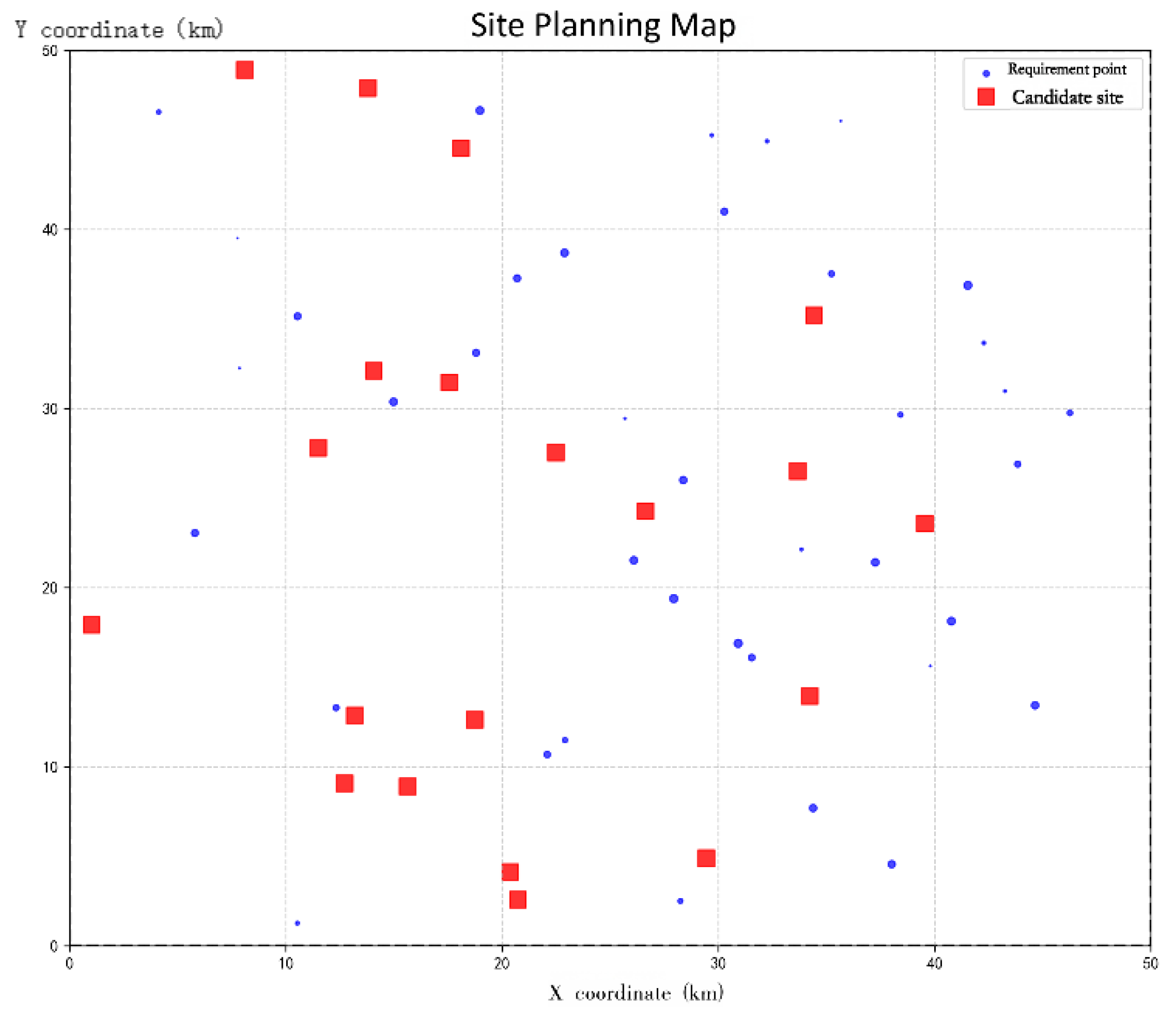
Figure 2.
The number of solutions for different sequences.
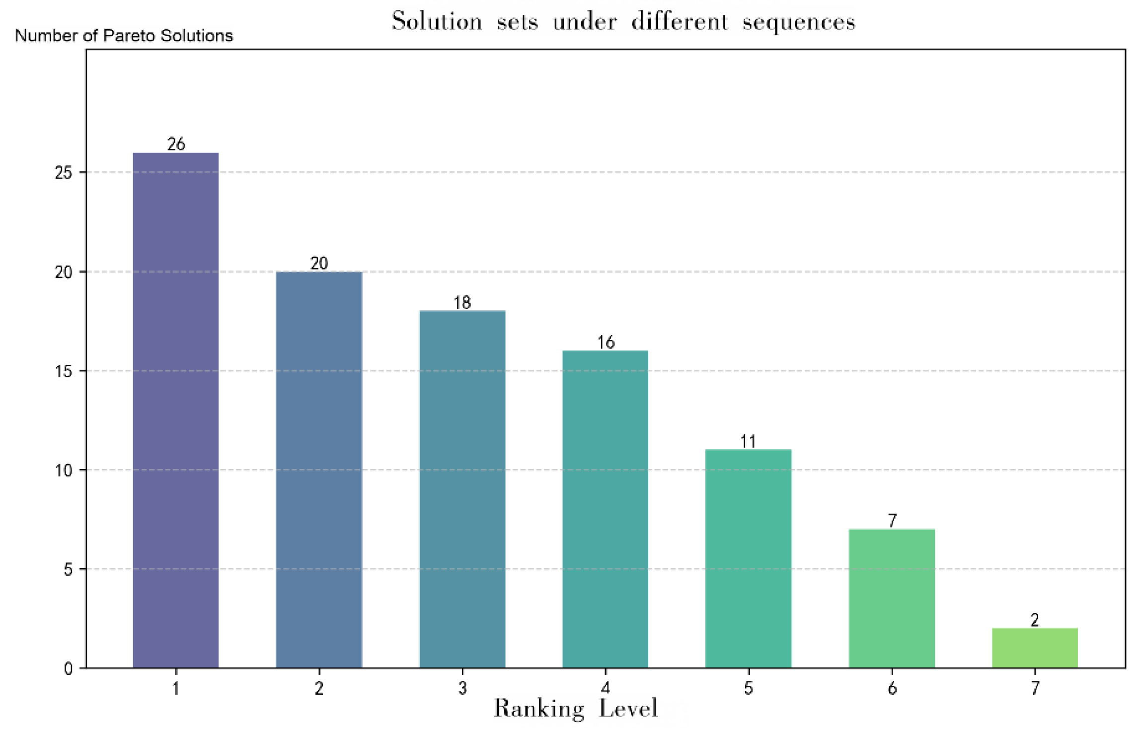
Figure 3.
The Pareto front solution set.
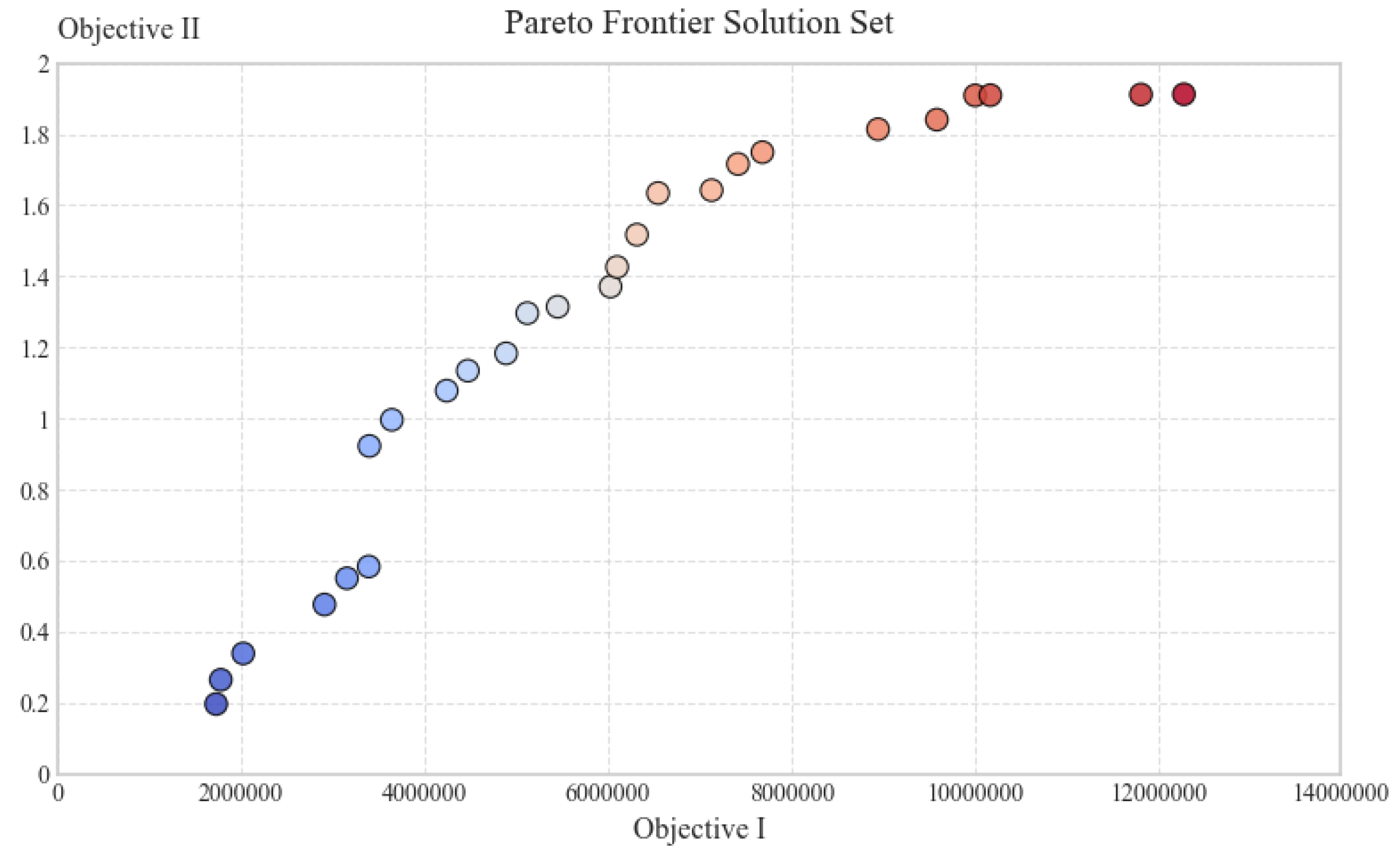
Figure 4.
Optimal site selection scheme based on the improved TOPSIS model.
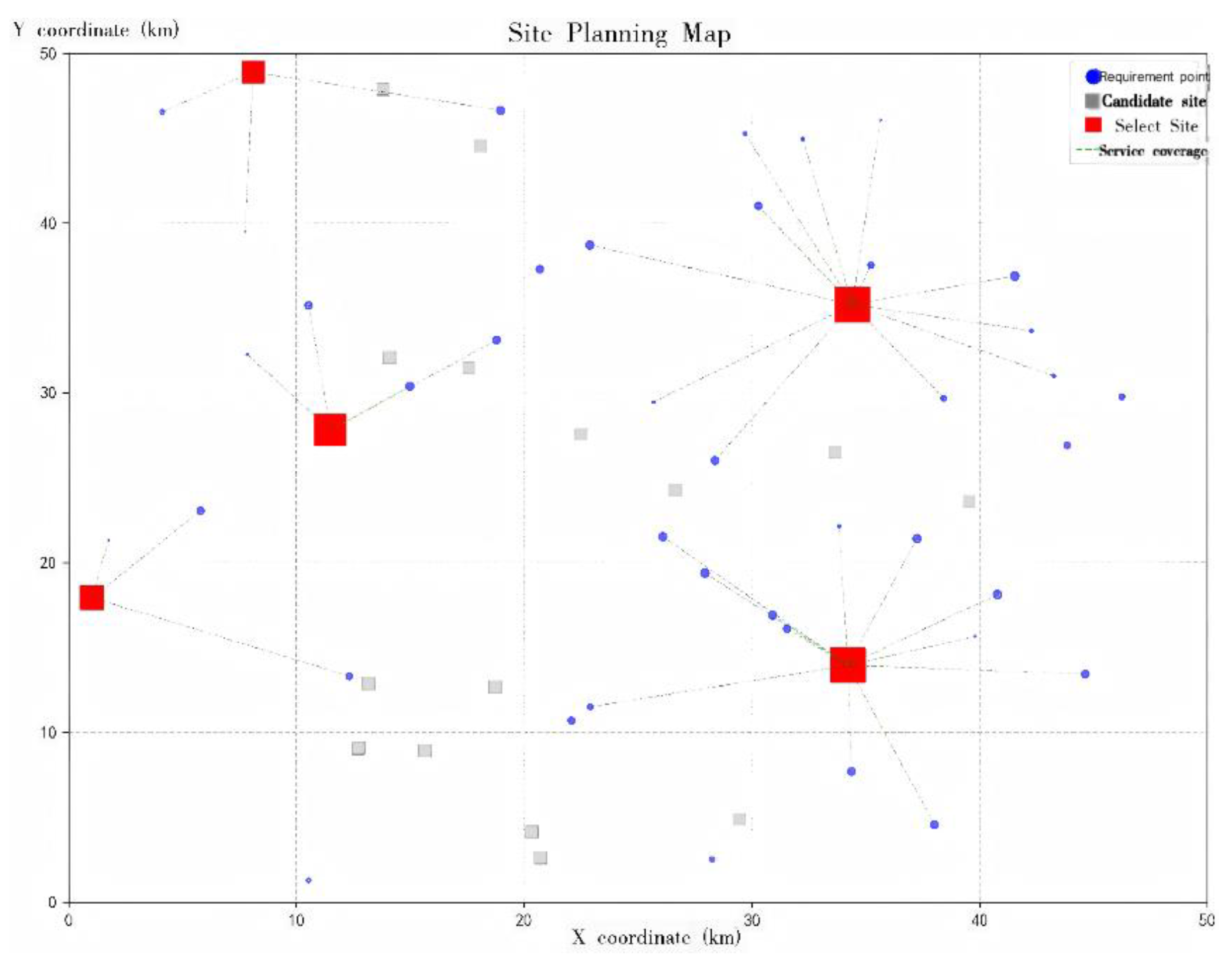
Figure 5.
Site selection scheme emphasizing operator cost minimization.
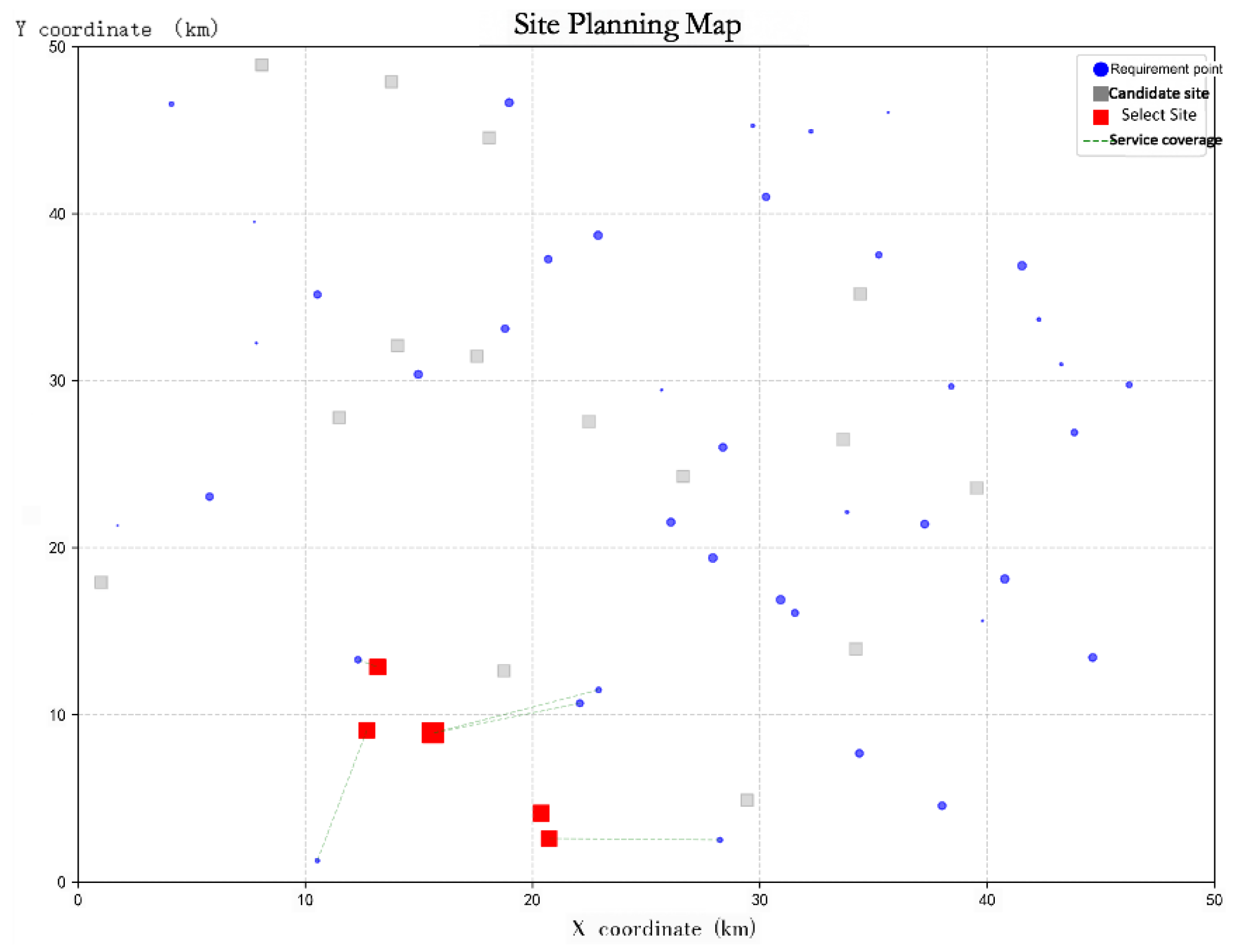
Figure 6.
Site selection scheme focusing on user satisfaction optimization.
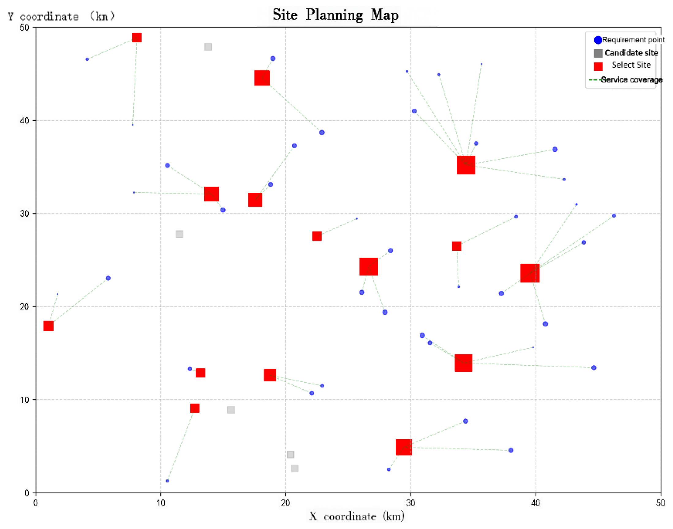
Figure 7.
Optimal site selection scheme based on the improved TOPSIS model.
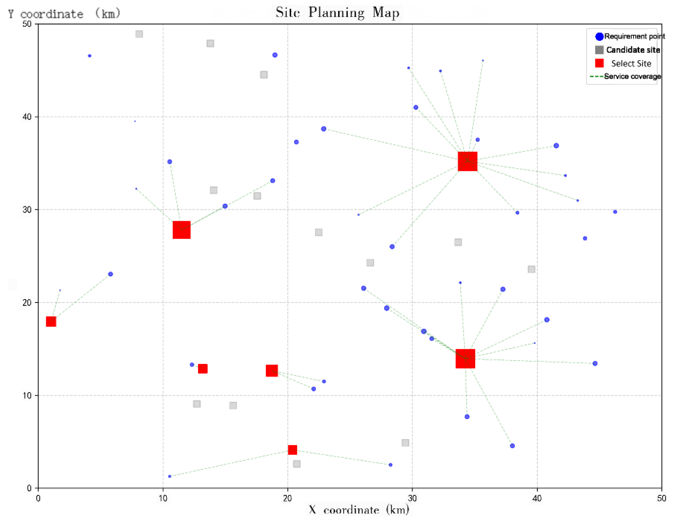
Table 1.
Demand and Coordinate Data of Demand Points.
| Numbering | X/km | y/km | Vehicle Demand/Vehicles | Numbering | X/km | y/km | Vehicle Demand/Vehicles |
|---|---|---|---|---|---|---|---|
| 1 | 18.98 | 46.63 | 43 | 26 | 1.75 | 21.32 | 1 |
| 2 | 38.43 | 29.65 | 19 | 27 | 10.54 | 1.27 | 11 |
| 3 | 5.80 | 23.04 | 36 | 28 | 10.54 | 35.14 | 35 |
| 4 | 7.86 | 32.24 | 2 | 29 | 38.02 | 4.55 | 39 |
| 5 | 35.66 | 46.05 | 2 | 30 | 32.25 | 44.92 | 9 |
| 6 | 9.73 | 9.80 | 12 | 31 | 30.92 | 16.88 | 48 |
| 7 8 9 10 11 12 13 14 15 16 17 18 19 20 21 22 23 24 25 |
30.36 14.98 3.24 22.89 25.68 42.28 4.12 39.80 33.84 30.28 44.65 37.26 28.25 38.21 29.70 28.38 41.54 40.78 7.76 |
1.34 30.37 47.74 38.69 29.44 33.65 46.55 15.62 22.13 40.99 13.42 21.41 2.50 46.10 45.25 26.00 36.87 18.12 39.50 |
25 42 15 44 3 9 14 2 7 35 40 42 18 36 8 40 47 45 1 |
32 33 34 35 36 37 38 39 40 41 42 43 44 45 |
18.80 36.02 27.94 35.24 12.33 26.09 22.09 31.55 34.38 20.70 46.26 43.26 22.91 43.84 |
33.10 31.60 19.38 37.52 13.29 21.52 10.68 16.09 7.69 37.27 29.75 30.97 11.49 26.89 |
37 47 27 26 27 42 32 32 39 26 22 6 20 8 |
Table 2.
Coordinate Locations of Candidate Sites.
| Numbering | X/km | y/km | Numbering | X/km | y/km |
|---|---|---|---|---|---|
| 1 | 18.10 | 44.53 | 11 | 34.42 | 35.19 |
| 2 | 14.06 | 32.09 | 12 | 8.11 | 48.89 |
| 3 | 1.02 | 17.92 | 13 | 13.81 | 47.88 |
| 4 | 15.63 | 8.90 | 14 | 20.73 | 2.59 |
| 5 | 26.64 | 24.27 | 15 | 17.56 | 31.45 |
| 6 | 34.24 | 13.93 | 16 | 33.67 | 26.48 |
| 7 8 9 10 |
12.72 11.50 20.38 13.19 |
9.08 27.79 4.11 12.85 |
17 18 19 20 |
22.49 29.45 18.74 39.55 |
27.54 4.88 12.62 23.57 |
Table 3.
Numerical Values of the Pareto Solution Set.
| Solution | Candidate Site Number | Number of Charging Piles | Objective Function I | Objective Function II |
|---|---|---|---|---|
| 1 |
2,6,8,9,10,11,12 | 20,20,6,4,4,20,8,7,20 | 10007068.4408 | 1.9092 |
| 2 | 1,2,3,5,6,7,10,11,12, 15,16,17,18,19,20 |
12,11,5,17,16,4,4,18, 4,10,4,4,13,7,9 |
12285334.7429 | 1.9124 |
| 3 |
4,7,9,10,14 | 7,4,4,4,4 | 1723119.1335 | 0.1961 |
| 4 |
4,10,14,16,19 | 4,4,4,7,20 | 3395770.3427 | 0.9224 |
| 5 |
3,7,8,9,13 | 5,5,16,10,18 | 3388560.6392 | 0.5831 |
| 6 |
1,3,6,7,8,9,11,12,13 | 17,5,20,5,16,10,20, 4,4 |
8947242.0281 | 1.8140 |
| 7 |
3,6,7,8,9,10,11,12,14 | 5,20,4,16,7,4,20,8, 4 |
7685543.9178 | 1.7492 |
| 8 |
19,11,8,10,7,12,15,1, 3,2,18,5,20,9,14 |
7,18,4,4,4,4,10,12,5, 11,13,20,20,4,4 |
11816704.0162 | 1.9117 |
| 9 |
3,6,7,9,10,12 | 5,20,4,10,4,18 | 4239305.6507 | 1.0781 |
| 10 |
3,4,6,7,9,11,14,19 | 11,5,20,4,20,8,4,16, 7,20 |
6099409.1505 | 1.4262 |
| 11 |
2,3,6,10,11,12,14,15, 19,20 |
11,5,20,4,20,8,4,16, 7,20 |
10172891.6210 | 1.9098 |
| 12 |
3,4,7,9,10 | 5,7,4,4,4 | 1773587.0580 | 0.2644 |
| 13 |
6,8,11,12,3 | 20,16,20,8,9 | 6546410.7668 | 1.6342 |
| 14 |
3,7,10,14,16,18 | 5,4,4,7,20,13 | 4470016.1623 | 1.1344 |
| 15 |
1,3,6,7,9,12,13 | 20,5,20,5,10,4,4 | 6027312.1157 | 1.3709 |
| 16 |
3,4,6,7,8,10,11,14 | 5,7,20,4,16,4,20,4 | 7130396.7493 | 1.6423 |
| 17 |
4,7,13,3,8 | 7,5,8,5,16 | 3150640.4241 | 0.5501 |
| 18 |
6,8,10,11,12 | 20,20,12,20,8 | 7418784.8888 | 1.7160 |
| 19 |
4,7,10,13,16 | 7,4,4,8,20 | 3640900.2613 | 0.9961 |
| 20 |
2,6,10,11,12,14,19,20 | 20,20,4,20,8,4,7,20 | 9588905.6385 | 1.8409 |
| 21 |
1,3,6,7,10 | 20,5,20,4,11 | 5450535.8366 | 1.3143 |
| 22 | 3,4,7,10,13 | 5,7,4,4,8 | 2018716.9765 | 0.3385 |
| 23 |
3,4,7,8,9 | 5,7,5,16,4 | 2905510.5055 | 0.4761 |
| 24 |
1,4,9,16,19 | 20,5,4,20,7 | 5118889.4762 | 1.2962 |
| 25 |
3,6,9,12,13,15 | 5,20,15,4,6,20 | 6315700.2552 | 1.5171 |
| 26 |
3,6,7,8,9,19 | 5,20,5,16,4,7 | 4888178.9646 | 1.1831 |
Table 5.
Comparison of Algorithm Search Performance.
| Performance Indicator | Enhanced NSGA-II | Standard NSGA-II | Performance Gain |
|---|---|---|---|
| Hypervolume | 16326381.9343 | 15665000.3202 | 4.222% |
| Inverted Generational Distance | 0.0245 | 0.0269 | 8.8652% |
| Diversity | 1.4630 | 1.0984 | 33.1887% |
| Runtime/s | 45.1924 | 38.9006 | -16.1741% |
Table 6.
Comparison of Ranking Results.
| Algorithm Type | Rank | TOPSIS Score | Total Operator Cost (10k CNY) | User Satisfaction | Candidate Site ID | Number of Charging Piles |
|---|---|---|---|---|---|---|
| Enhanced NSGA-II | 1 | 0.7003 | 6546410.7668 | 1.6342 | 6,8,11,12,3 | 20,16,20,8,9 |
| Standard NSGA-II | 1 | 0.6928 | 6820379.4993 |
1.6426 |
2,5,7,8,9,10, 18 |
5,20,16,4,4,20, 7 |
Disclaimer/Publisher’s Note: The statements, opinions and data contained in all publications are solely those of the individual author(s) and contributor(s) and not of MDPI and/or the editor(s). MDPI and/or the editor(s) disclaim responsibility for any injury to people or property resulting from any ideas, methods, instructions or products referred to in the content. |
© 2025 by the authors. Licensee MDPI, Basel, Switzerland. This article is an open access article distributed under the terms and conditions of the Creative Commons Attribution (CC BY) license (https://creativecommons.org/licenses/by/4.0/).
Copyright: This open access article is published under a Creative Commons CC BY 4.0 license, which permit the free download, distribution, and reuse, provided that the author and preprint are cited in any reuse.


