Submitted:
11 December 2025
Posted:
12 December 2025
You are already at the latest version
Abstract
For the hierarchical normal and normal-inverse-gamma model, we derive the Bayesian estimator of the variance parameter in the normal distribution under Stein's loss function---a penalty function that treats gross overestimation and underestimation equally---and compute the associated Posterior Expected Stein's Loss (PESL). Additionally, we determine the Bayesian estimator of the same variance parameter under the squared error loss function, along with its corresponding PESL. We further develop empirical Bayes estimators for the variance parameter using a conjugate normal-inverse-gamma prior, employing both the method of moments and Maximum Likelihood Estimation (MLE). Through numerical simulations, we examine five key aspects: (1) the consistency of moment-based and MLE-based hyperparameter estimators; (2) the influence of κ₀ on quantities of interest as functions of the most recent observation; (3) two inequalities involving the Bayesian estimators and their respective PESL values; (4) the model's goodness-of-fit to simulated data; and (5) graphical representations of marginal densities under different hyperparameter settings. The simulation results demonstrate that MLEs outperform moment estimators in estimating hyperparameters, particularly with respect to consistency and model fit. Finally, we apply our methodology to real-world data on poverty levels---specifically, the percentage of individuals living below the poverty line---to validate and illustrate our theoretical findings.
Keywords:
empirical bayes estimators
; hierarchical normal and normal-inverse-gamma model
; maximum likelihood estimation (MLE) method
; moment method
; stein’s loss function
MSC: 62C12; 62F10; 62F15
1. Introduction
The empirical Bayes method depends on a conjugate prior modeling, where the hyperparameters are estimated from the observations and the “estimated prior" is then used as a regular prior in the subsequent inference. See [1,2,3] and the references therein. The empirical Bayes method is introduced in [4,5,6]. From Bayesian perspective, it means that the sampling distribution is known, but the prior distribution is not. The marginal distribution is then used to restore the prior distribution from the observations. More literature on empirical Bayes method can be found, for instance, in [7,8,9,10,11,12,13,14,15,16,17,18,19,20,21,22,23,24].
The motivations of this paper are summarized as follows. Example 1.5.1 (p.20) of [25], Part I (pp.69-70) of [26], and [19] have considered the following hierarchical normal and normal-inverse-gamma model:
where , , , and are known hyperparameters, and iid means independent and identically distributed. The distribution is a joint conjugate prior for of the normal distribution , so that the posterior distribution of is an distribution with updated hyperparameters. However, in reality, the hyperparameters are unknown. [19] have estimated the hyperparameters of the model (1) by the moment method and the Maximum Likelihood Estimation (MLE) method. Moreover, they obtained the Bayes estimators of the mean and variance parameters of the model (1) under the squared error loss function. Finally, they obtained the empirical Bayes estimators of the mean and variance parameters of the model (1) under the squared error loss function by the moment method and the MLE method. However, in their empirical Bayes estimators, the sample have been used twice. First, the sample are utilized to estimate the hyperparameters , , , and . Second, the sample are used to obtain the Bayes estimators. To avoid using the sample twice, and to be compatible with the usual empirical Bayes analysis, we will use the following hierarchical normal and normal-inverse-gamma model in this paper:
where , , , and are hyperparameters to be determined, and are the unknown parameters of interest, is a normal distribution with an unknown mean and an unknown variance , the conditional conjugate prior distribution of given is which is a normal distribution with mean and an unknown variance , the marginal conjugate prior distribution of is which is an inverse gamma distribution with shape parameter and scale parameter . Note that the joint conjugate prior is a normal-inverse-gamma distribution. As described in [7], the statistician observes data and wishes to make an inference about and . Therefore, provides direct information about the parameters and , while supplementary information is also available. The connection between the prime data and the supplementary information is provided by the common distributions , , and . Moreover, since the variance parameter of the normal distribution is a positive restricted parameter, the squared error loss function is not appropriate. In contrast, we will choose Stein’s loss function because it penalizes gross overestimation and gross underestimation equally, that is, an action a will incur an infinite loss when it tends to 0 or ∞. Note that the squared error loss function does not have this property. For more literature on Stein’s loss function, we refer readers to [20,27,28,29,30].
The key contributions of this work are outlined below. For the hierarchical normal and normal-inverse-gamma (N-NIG) framework (2), we begin by deriving the posterior distributions and marginal density, as stated in Theorem 1. Subsequently, we derive Bayes estimators for the variance parameter of the normal distribution under two loss criteria: Stein’s loss and the squared error loss. We further compute the corresponding Posterior Expected Stein’s Losses (PESLs) associated with these two estimators. It is shown that the two Bayes estimators and their respective PESLs satisfy specific inequalities, namely (15) and (16). Additionally, we derive moment-based estimators for the hyperparameters of the N-NIG model (2) and establish their consistency in Theorem 2. Similarly, Maximum Likelihood Estimators (MLEs) for the same hyperparameters are derived, and their consistency is proven in Theorem 3. Building on these results, we construct empirical Bayes estimators for the variance parameter under Stein’s loss using both the method of moments and MLE, as presented in Theorem 4. The theoretical findings are supported by numerical experiments and an application to real-world data.
Comparing models (1) and (2) carefully, we find that the samples and generated from the two models are iid from different distributions. On the one hand, the sample generated from (1) are iid from . Although the marginal densities of are , and thus can be thought to be from the t distribution. However, are not iid from the t distribution. In other words, are dependent from the t distribution. On the other hand, the sample generated from (2) are iid from the t distribution. That is, are independent and identically distributed from the t distribution. The sample can be used to estimate the parameters and from , while the sample can be used to estimate the hyperparameters , , and from , where .
The structure of this paper is outlined as follows. Section 2 begins with the derivation of posterior distributions and the marginal likelihood for the hierarchical normal and normal-inverse-gamma model. Subsequently, we derive the corresponding Bayes estimators and PESLs, which are shown to fulfill two key inequalities: (15) and (16). Additionally, Theorem 4 presents the empirical Bayes estimators for the model’s variance component under Stein’s loss function, obtained via both the method of moments and MLE. In Section 3, we conduct numerical experiments from five different perspectives to evaluate performance. Section 4 illustrates the methodology using real-world data, specifically poverty rate data reflecting the proportion of individuals living below the poverty line. Finally, Section 5 offers concluding remarks and a discussion of the findings.
2. Theoretical Results
Suppose that and . The probability density functions (pdfs) of X and Y are respectively given by
It is easy to calculate and , for and .
2.1. The Bayes Estimators and the PESLs
For the hierarchical normal and normal-inverse-gamma model (2), we have the following theorem which calculates the posterior densities , , , , and the marginal density . The proof of the theorem can be found in the Appendix A.
Theorem 1.
For the hierarchical normal and normal-inverse-gamma model (2), the joint posterior density of is
the marginal posterior density of is
the marginal posterior density of is
the conditional posterior density of is
where
and
Moreover, the marginal density of is given by
with probability density function (pdf) given by
for , , , , and .
In the following, we will calculate the Bayes estimator of under Stein’s loss function , the Bayes estimator of under the usual squared error loss function , and the PESLs at and ( and ).
To calculate the two Bayes estimators and the two PESLs, it remains to calculate
Similar to [28], it can be shown that
by exploiting Jensen’s inequality. Moreover,
which is a direct consequence of the general methodology for finding a Bayes estimator. According to construction, minimizes the Posterior Expected Stein’s Loss (PESL).
Now let us analytically calculate the Bayes estimators and , and the PESLs and under the hierarchical normal and normal-inverse-gamma model (2) from (7), (8), (9), and (10). The three expectations are calculated as
for , where and are given by (4) and (5). From (7), the Bayes estimator of under Stein’s loss function is given by
From (8), the Bayes estimator of under the usual squared error loss function is given by
for . It is easy to show that
which exemplifies the theoretical study of (11). Furthermore, from (9) and (10), the PESL at and are respectively given by
and
where
is the digamma function. It can be shown that
which exemplifies the theoretical study of (12). It is worth noting that the PESLs and depend only on , but not on . Therefore, the PESLs depend only on , but not on , , , and .
2.2. The Empirical Bayes Estimators of
The hyperparameters of model (2) are , , , and . However, we can not directly obtain the estimators of the four hyperparameters of model (2) by the moment method. Let
Since and appear together in , we can not directly obtain the estimators of and by the moment method. In other words, and are unidentifiable. In the empirical Bayesian statistical literature, common approaches to addressing the issue of unidentifiability of hyperparameters include the following two. One is to estimate the prior distribution through non-parametric or semi-parametric methods, avoiding strong assumptions about the functional form of the prior distribution, thereby circumventing the problem of unidentifiability of hyperparameters ([31,32]). The other is to use auxiliary data, model structure constraints, or specific assumptions (such as sparsity, spatial correlation) to provide additional information, making the unidentifiable hyperparameters identifiable ([33,34,35]). We adopt the second approach to make hyperparameters ( and ) identifiable. More specifically, when is fixed to be a known constant (our recommendation is , which will be made clear later in this subsection), then and are identifiable. Otherwise, and are unidentifiable.
However, we can obtain the estimator of by the moment method. In the following, we are interested in the hyperparameters , , and . Using hyperparameters , , and , the marginal density (6) changes to
The moment-based estimators for the hyperparameters , , and in model (2), denoted as , , and , along with their consistency properties, are presented in the subsequent theorem. The proof of this theorem is provided in the Appendix A.
Theorem 2.
The estimators of the hyperparameters , , and of model (2) by the moment method are
where
is the sample kth moment of X. Moreover, the moment estimators are consistent estimators of the hyperparameters.
We remark that the moment estimators , , and in Theorem 2 are the same as those in Theorem 2 in [19]. The reason for the same moment estimators is that for the two hierarchical normal and normal-inverse-gamma models (1) and (2), the marginal distributions are the same, and the population moments of X are the same. Moreover, in Theorem 2 of this paper, we have shown that the moment estimators are consistent estimators of the hyperparameters, and this result has not been derived in [19].
The MLE method is used to derive estimators for the hyperparameters , , and of the model (2), denoted as , , and , respectively. The consistency properties of these estimators are presented in the subsequent theorem, with the detailed proof provided in the Appendix A.
Theorem 3.
The estimators of the hyperparameters , , and of the model (2) by the MLE method , , and are the solutions to the following equations:
Moreover, the MLEs are consistent estimators of the hyperparameters.
The MLEs of the hyperparameters , , and cannot be derived analytically by solving equations (19), (20), and (21). As a result, numerical methods must be employed. Newton’s method can be applied to solve these equations and thereby obtain the MLEs of the hyperparameters. It should be emphasized that the accuracy of the resulting MLEs is highly sensitive to the choice of initial values, and moment-based estimators have generally been found to serve as effective starting points.
Finally, the empirical Bayes estimates of the model (2)’s variance parameter under Stein’s loss function, derived using the method of moments and the MLE, are presented in the subsequent theorem.
Theorem 4.
The empirical Bayes estimator of the variance parameter of the model (2) under Stein’s loss function by the moment method is given by (13) with the hyperparameters estimated by in Theorem 2. Alternatively, the empirical Bayes estimator of the variance parameter of the model (2) under Stein’s loss function by the MLE method is given by (13) with the hyperparameters estimated by numerically determined in Theorem 3.
Now let us discuss the selection of . We recommend choosing , and the reason is given as follows. From (13), (4), and (5), we have
It is easy to show that the factor
for . Because we have little information about , we will choose
which is in the middle of the above range. Hence,
Therefore, (22) reduces to
which can then be estimated once the hyperparameters are estimated. From (17) and (23), we have
which can then be estimated once the hyperparameter is estimated.
Another reason to choose is given below. Since , the squared error loss function is appropriate. The Bayes estimator of under the squared error loss function is given by
In (24), represents a strength of belief on . If one harbors no belief on , then , and thus , which depends only on the datum . In contrast, if one harbors complete belief on , then , and thus , which depends only on . However, if one believes that and are equally important, then is a reasonable choice, and thus , which is a balanced combination of and .
We remark that and affect , , , and , and they do not affect , , and .
3. Simulations
This section presents numerical simulations for the hierarchical normal and normal-inverse-gamma model (2). We examine five key aspects: the consistency of moment estimators and MLEs, the influence of on quantities of interest as functions of , the validity of two inequalities concerning Bayes estimators and PESLs, the model’s goodness-of-fit to the generated data, and the marginal density distributions of the model parameters.
The simulated data are generated according to the hierarchical normal and normal-inverse-gamma model (2) with the hyperparameters specified by , , , and . The reason why we choose these values is that , , , and . Moreover, is required in moment estimations of the hyperparameters. Additional numerical values for the hyperparameters can likewise be defined.
3.1. Consistencies of the Moment Estimators and the MLEs
Currently, both the moment estimators and the MLEs serve as consistent estimates for the hyperparameters of the hierarchical normal and normal-inverse-gamma model (2). The purpose of this subsection is to emphasize that, as established in Theorems 2 and 3, we have rigorously proven the consistency of both the moment-based and MLE-based estimators with respect to the true hyperparameters. It should be noted that all analyses here are based solely on the observed data .
First, we will numerically exemplify that the sample generated from the model (1) can not be used to estimate the hyperparameters , while the sample generated from the model (2) can be used to estimate the hyperparameters , where . Moreover, we will exemplify that the moment estimators and the MLEs of can correctly estimate the true hyperparameter regardless of the and values.
The histograms of the samples and their density curves are plotted in Figure 1. From the figure, we observe the following facts.
- Plot (a): the sample generated from (1) are iid from with and .
The moment estimators and the MLEs of the hyperparameters for the samples , , and are summarized in Table 1. From the table, we observe the following facts.
- The moment estimators of the hyperparameters for sample are far away from the true hyperparameters , and thus the samples generated from the model (1) can not be used to estimate the hyperparameters .
- For , since the moment estimator of is which is negative, the MLE method fails to iterate, and thus the MLEs of the hyperparameters are equal to the moment estimators.
- For and , the moment estimators and the MLEs of the hyperparameters are close to the true hyperparameters , and thus the samples generated from the model (2) can be used to estimate the hyperparameters .
- For and , the MLEs are closer to the true hyperparameters than the moment estimators for this simulation.
Following the approach in [21], let represent one of the hyperparameters , , or . Consistency is defined as the property that
for , where corresponds to the moment estimator and to the MLE, with denoting convergence in probability and n being the sample size. Equivalently, consistency can be expressed as
for any and for all . These probabilities are estimated using empirical frequencies from simulations:
where is the indicator function taking value 1 if event A occurs and 0 otherwise, and M denotes the number of simulation replications. Hence, a decreasing trend in the simulated frequencies toward zero as n increases provides empirical evidence of estimator consistency, for both estimation methods () and across all hyperparameters .
We now demonstrate that the moment estimators and the MLEs are consistent estimators of the hyperparameters . Table 2 presents the frequency distributions of these estimators for both moment-based and MLE for varying sample sizes n, under settings where , , and . The simulated data are generated from the hierarchical normal and normal-inverse-gamma model (2), with hyperparameter values set to and . While other configurations of these hyperparameters could also be considered, the current choice serves to illustrate the behavior effectively. Analysis of the table reveals several key observations.
- With , , or , the frequencies of the estimators approach zero as n tends to infinity, indicating that both the moment estimators and the MLEs are consistent for estimating the hyperparameters. In the case of , the frequencies of and remain relatively high (at least across all scenarios). Nevertheless, a decreasing trend toward zero is evident as n grows large, suggesting eventual convergence.
- By comparing the frequencies corresponding to , , and , we find that as decreases, the frequencies generally increase. This occurs because the constraintsbecome easier to satisfy when is smaller.
- When comparing the moment estimators with the MLEs of the hyperparameters , , and , it is observed that for large sample sizes n, the MLEs exhibit smaller values than the moment estimators. This indicates that, in terms of consistency, the MLEs perform more reliably in estimating the hyperparameters.
3.2. The Effect of for Quantities of Interest as Functions of
In this subsection, we will investigate the effect of for quantities of interest (, , , , , , and ) as functions of . The motivation of this subsection is that is unidentifiable, and we want to know whether using (our recommendation) for the computation will overestimate or underestimate quantities of interest as functions of when the true (e.g., 2 or ) is different from .
Quantities of interest as functions of for in the simulations are plotted in Figure 2. In all the plots, is fixed. From the figure, we observe the following facts.
- From the left column of the figure, we see that , , , and are affected by . Moreover, , , and are quadratic functions of (note that their y ranges are different), while is a linear function of .
- For plot (a), we observe that when using will underestimate when using , and it will overestimate when using . In other words, is an increasing function of for a fixed . Similar phenomena are observed for (plot (c)) and (plot (e)).
- For (plot (g)), we observe an interesting phenomenon that when ( in the simulation), when using will underestimate that when using , and it will overestimate that when using . In other words, is an increasing function of when . However, when , we observe a reversed phenomenon that when using will overestimate that when using , and it will underestimate that when using . In other words, is a decreasing function of when . The phenomena can be explained by the theoretical analysis of
- From the right column of the figure, we see that , , and are not affected by . Moreover, they also do not depend on .
3.3. Two Inequalities of the Bayes Estimators and the PESLs
This subsection aims to provide numerical illustrations of the two inequalities related to the Bayes estimators and the PESLs—specifically, (15) and (16)—under the oracle scenario where the hyperparameters are known. The rationale for this section lies in the theoretical foundation established by these two inequalities, which we seek to validate through numerical examples.
First, we fix , , , and . Then we set a seed number 1 in R software and draw from . Next, we draw from . After that, we draw from . Figure 3 shows the histogram of and the density estimation curve of . It is that we find to minimize the PESL. Numerical results show that
and
which exemplify the theoretical studies of (15) and (16).
We now consider the scenario where one of the five parameters—, , , , and —is allowed to vary while the others remain constant. Specifically, our focus lies on conducting a sensitivity analysis of the Bayes estimators and the PESLs with respect to these five parameters.
Figure 4 illustrates the Bayes estimators and the PESLs as varying with . As shown in the left panel, the Bayes estimators exhibit dependence on , demonstrating the validity of inequality (15). Specifically, increases as increases, whereas decreases with rising . The right panel reveals that the PESLs are also influenced by , supporting the inequality (16), and both PESLs decrease monotonically as grows. Additionally, numerical values corresponding to these quantities are provided in Table 3, which aligns with the graphical representation in Figure 4. Overall, both the figure and the table confirm the two theoretical inequalities: (15) and (16).
Figure 5 shows the Bayes estimators and the PESLs as functions of , , , and . We see from the left plots of the figure that the Bayes estimators depend on , , , and , and (15) is exemplified. Moreover, the Bayes estimators are first decreasing and then increasing functions of and , and they are increasing functions of and . The right plots of the figure exhibit that the PESLs do not depend on , , , and , and (16) is exemplified. Furthermore, Table 4, Table 5, Table 6 and Table 7 display the numerical values of the Bayes estimators and the PESLs in Figure 5. In summary, the results of Figure 5 and Table 4, Table 5, Table 6 and Table 7 exemplify the two inequalities (15) and (16).
In brief, the results of Figure 4 and Figure 5 exemplify that the PESLs depend only on , but not on , , , and .
Since the estimators and , along with their corresponding PESLs— and —are functions of the parameters and , where and , we visualize their behavior across the domain using the persp3d() function from the R package rgl (refer to [20,21,36,37]). A key advantage of persp3d() over the standard persp() function in the graphics package is its ability to overlay multiple surfaces within the same plot and enable interactive rotation of 3D visualizations, thereby offering greater flexibility in graphical analysis. The resulting surface plots for the estimators, the PESLs, and their pairwise differences are displayed in Figure 6. As shown in the two leftmost panels, consistently exceeds across all values of , providing empirical support for the inequality stated in (15). Similarly, the rightmost panels indicate that remains greater than throughout D, which visually confirms the theoretical result in (16). Overall, the numerical illustrations in the figure corroborate the analytical findings presented in (15) and (16).
3.4. Goodness-of-Fit of the Model: KS Test
This section focuses on evaluating the goodness-of-fit of the hierarchical normal and normal-inverse-gamma model (2) to the generated synthetic data. The primary objective is to assess how well the marginal distribution of the N-NIG model captures the characteristics of the simulated dataset. It should be noted that the analysis here is based solely on the observed data points .
The Kolmogorov-Smirnov (KS) statistic measures the maximum discrepancy, denoted as D, between the empirical cumulative distribution function (cdf), , and the theoretical population cdf, . Mathematically, this is expressed as
In R, the KS test can be carried out using the built-in function ks.test() (refer to [38,39,40]). While the standard KS test is primarily designed for one-dimensional continuous distributions, various adaptations known as KS-type tests have also been proposed in the literature for handling discrete data ([41,42,43]).
The R function ks.test() performs the KS test, and its return value is a list containing the components statistic (the value of the test statistic, or the D value) and p.value (the p-value of the test). In the literature, it is well known that a smaller D value or a larger p-value indicates a better fit of the model to the simulated data. Based on and inspired by the D value and p-value, [21] propose five indices (, , , , ) to compare the three methods, that is, the oracle method, the moment method, and the MLE method in simulations. is the average D values (25) of M simulations (the smaller the better). is the average p-values of M simulations (the larger the better). is the percentage of M simulations which attain the minimum D value in the three methods (the larger the better). The three values should sum to 1. is the percentage of M simulations which attain the maximum p-value in the three methods (the larger the better). The three values should sum to 1. is the percentage of accepting (defined as p-value ) in M simulations for each method (the larger the better). Each value should between .
In our problem, the null hypothesis specifies that
where is the marginal distribution of the hierarchical normal and normal-inverse-gamma model (2). The marginal density of the distribution is given by (18) which is obviously one-dimensional and continuous. Therefore, the KS test can serve as an indicator of how well the model fits the data.
It should be noted that the data presented in this section are generated based on the hierarchical normal and normal-inverse-gamma model (2), where the hyperparameters are set to and . Alternative values for these hyperparameters may also be chosen depending on the context.
Table 8 presents the goodness-of-fit results from the KS test for model (2) applied to simulated data. The simulations are based on a sample size of and repeated times. Hyperparameter estimation for , , and is conducted using three distinct approaches. The first is the oracle method, which assumes prior knowledge of the true values: , , and . The second approach employs the method of moments, utilizing moment estimators derived in Theorem 2. The third approach relies on MLE, where the hyperparameters are numerically computed using the MLEs provided in Theorem 3.
As shown in Table 8, the following observations can be made.
- The values corresponding to the three approaches are , , and , respectively. This indicates that the MLE method performs best, followed by the moment method, while the oracle method yields the least satisfactory results. A plausible explanation for this outcome is that, as shown in (25), the empirical cdf relies on observed data, and similarly, the theoretical cdf used in both the moment and MLE methods are derived from data. In contrast, the associated with the oracle method does not depend on actual data.
- The corresponding to the three methods are , , and , respectively, indicating that the MLE method performs best, followed by the moment method, with the oracle method ranking last. A plausible explanation for this outcome is provided in the preceding paragraph.
- The values for the three approaches are , , and , respectively. For the MLE method, the value exceeds half of the M simulations. In terms of performance ranking, the methods are ordered as follows: MLE method, oracle method, and moment method.
- The three methods yield values of , , and , respectively. Since a lower D value is associated with a higher p-value, the method producing the minimum D value will also produce the maximum p-value. As a result, the and values are identical across the three approaches. Based on performance, the methods can be ranked in descending order of preference as follows: MLE method, oracle method, and moment method.
- The values for the three methods are , , and , respectively, indicating that these values are close to . This suggests that all three methods exhibit strong performance in terms of model fit.
- To summarize, the MLE method consistently achieves the top ranking across all five evaluation metrics—, , , , and . When comparing the moment method with the MLE method, the results indicate that the MLE method outperforms the moment method on each of these five criteria.
Figure 7 presents the boxplots of the D values and p-values obtained from the three methods. The following observations can be made based on this figure.
- The D values obtained by the oracle method are higher than those of the other two approaches. Since lower D values indicate better performance, the preferred ranking of the three methods is as follows: MLE method, moment method, and then the oracle method.
- The oracle method yields the lowest p-values compared to the other two approaches. Since higher p-values are preferable, the methods can be ranked in descending order of preference as follows: MLE method, moment method, and finally the oracle method.
- Large D values are associated with small p-values, whereas small D values are linked to large p-values.
- Based on the D values and p-values, the MLE method outperforms the method of moments.
3.5. Marginal Densities for Various Hyperparameters
This subsection presents the marginal density plots of the hierarchical normal and normal-inverse-gamma model (2) under different settings of the hyperparameters , , , and . The primary objective is to investigate the types of data distributions that can be captured by this hierarchical model. Recall that the marginal density of X is defined by equation (6), which depends on four hyperparameters: (ranging over the real line), , , and . Our analysis focuses on how variations in these hyperparameters affect the shape of the marginal density, using the baseline configuration , , , and as a reference point. Alternative values for the hyperparameters may also be considered to further explore the model’s flexibility.
Figure 8 displays the marginal density functions under different values of , with , , and held constant. It can be observed that as increases, the entire distribution shifts rightward without altering its shape, indicating that acts as a location parameter. Furthermore, each marginal density is symmetric around its corresponding mean value .
Figure 9 illustrates the marginal density functions under different values of , with , , and held constant. It can be observed that as grows larger, the peak of the marginal density becomes more pronounced, indicating a reduction in its spread. This is consistent with the theoretical expression for the variance of X, given by
which decreases as increases. Additionally, each marginal density remains symmetric around the common mean .
Figure 10 displays the marginal density functions under different values of , with , , and held constant. It can be observed that as grows larger, the height of the density peak rises, indicating a reduction in the spread of the distribution. This is consistent with (26), which shows that the variance of the marginal density decreases as increases. Additionally, each marginal density exhibits symmetry around the common mean .
Figure 11 displays the marginal density functions under different values of , with , , and held constant. As observed in the plot, an increase in leads to a reduction in the height of the density peak, indicating a broader distribution. This reflects a larger variance in the marginal density, which aligns with (26) showing that variance increases with . Additionally, each marginal density remains symmetric around the mean value .
4. A Real Data Example
In this section, we exploit the poverty level data. The data represent percentages of all persons below the poverty level. The sample is from a random collection of cities in the Western U.S. Source: County and City Data Book 12th edition, U.S. Department of Commerce. The data can be downloaded from
under section title “Poverty Level". Note that there is an “_" between understandable and statistics.
The histogram of the sample and its density estimation curveis depicted in Figure 12. From the figure, we see that the data are roughly symmetric about .
The estimators of the hyperparameters , , and , the goodness-of-fit of the model, the empirical Bayes estimators of the variance parameter of the normal distribution with a conjugate normal-inverse-gamma prior and the PESLs, and the mean and variance of the real data by the moment method and the MLE method are summarized in Table 9. From the table, we observe the following facts.
- The moment estimator of the hyperparameter is equal to the sample mean of the first n observations. It is worth noting that the MLE of the hyperparameter is equal to , which is very close to the moment estimator of the hyperparameter . Furthermore, the moment estimator and the MLE of the hyperparameter are also very similar, and they are close to . However, the moment estimator and the MLE of the hyperparameter are quite different. This does not mean that the moment estimator and the MLE are not consistent estimators of the hyperparameter , nor mean that the hierarchical normal and normal-inverse-gamma model (2) does not fit the real data. For the big difference between the two estimators, the reason is that the sample size is small. Certainly, the MLE of the hyperparameter is more reliable, as guaranteed from the previous figures and tables in the simulations section.
- The KS test is used as a measure of the goodness-of-fit. The p-value of the moment method is , which implies that the distribution with , , and estimated by their moment estimators fits the sample well. Moreover, the p-value of the MLE method is , which implies that the distribution with , , and estimated by their MLEs fits the sample even better. Comparing the moment method and the MLE method, we observe that the D value of the MLEs is smaller, and the p-value of the MLEs is larger, which means that the distribution with the hyperparameters , , and estimated by the MLEs has a better fit to the sample than that estimated by the moment estimators.
-
When the hyperparameters are estimated by the MLE method, we see thatand
- The mean of X (the poverty level data) is estimated by . The variance of X is estimated by . It is useful to note that the mean and variance of X by the two methods are very similar, although the estimators of the hyperparameters are very different. Moreover, it is worth mentioning thatfor the MLE method. For the moment method, the mean and variance of X are similar. Hence, the variance of X is very small, not large!
5. Conclusions and Discussions
For the hierarchical normal and normal-inverse-gamma (2) framework, we begin by deriving the posterior distributions , , , and , along with the marginal distribution , as presented in Theorem 1. Subsequently, we obtain the Bayes estimators and , as well as the corresponding PESLs, denoted by and . These quantities fulfill two key inequalities, given in (15) and (16). Additionally, Theorem 2 provides the moment-based estimates for the model’s hyperparameters—specifically , , and . In parallel, Theorem 3 summarizes the MLEs of the same hyperparameters, namely , , and . Lastly, Theorem 4 compiles the empirical Bayes estimators for the model’s variance component under Stein’s loss function, derived using both estimation approaches.
In the simulation study, we conduct numerical experiments on the hierarchical normal and normal-inverse-gamma model (2) from five perspectives: the consistency of moment estimators and MLEs, the influence of on quantities of interest as functions of , the validation of two inequalities related to Bayes estimators and PESLs, the model’s goodness-of-fit to the generated data, and the examination of the model’s marginal density distributions.
In the real data analysis, we utilize poverty level data reflecting the proportion of individuals living below the poverty threshold. Table 9 presents a summary of several key results: estimates of the hyperparameters , , and ; model goodness-of-fit measures; empirical Bayes estimates for the variance parameter under a normal distribution with a conjugate normal-inverse-gamma prior; PESL values; as well as the mean and variance estimates of the poverty data computed via both the method of moments and MLE. The MLE-based estimates demonstrate a superior fit to the observed sample compared to moment-based estimates, as evidenced by a smaller D statistic and a higher corresponding p-value, indicating that the distribution using MLE-derived hyperparameters better captures the characteristics of the data.
In empirical Bayes approaches, hyperparameters are treated as unknown quantities, and their estimation relies on the marginal distribution derived from observed data. Two widely used techniques for this purpose are the method of moments and MLE. This study applies both methods to estimate the hyperparameters within a hierarchical normal and normal-inverse-gamma model (2).
The simulation results presented in the preceding figures and tables demonstrate that MLEs outperform moment-based estimators in estimating the hyperparameters , , and , particularly with respect to consistency and model fit. Nevertheless, these advantages come at a cost. Unlike moment estimators, MLEs are prone to numerical instability, impose higher computational demands, necessitate the constraints and throughout all iterations, and lack closed-form solutions. Importantly, the performance of MLEs is highly sensitive to the choice of initial values, and moment estimators have been empirically shown to serve as reliable starting points. Furthermore, in scenarios where MLEs fail to converge or do not exist, moment estimators provide a justifiable and robust alternative.
Finally, we outline potential directions for future research. One possible extension involves adapting the hierarchical normal and normal-inverse-gamma model (2) to accommodate various non-conjugate prior distributions for the parameters of the normal distribution (refer to [1,44,45] and related works). In these cases, closed-form solutions may not be feasible, necessitating the development of numerical methods to compute the corresponding estimators.
Funding
This study was funded by the National Natural Science Foundation of China (Grant No. 12461051).
Conflicts of Interest
The author declares no conflict of interest.
Appendix A. Proofs of Theorems
In the appendix, we will provide some proofs of the theorems.
Appendix A.1. The Proof of Theorem 1
Let be the hyperparameters. The marginal distribution of in model (2) is
To lighten notations, the will be dropped in the densities. Some of the following derivations are quoted from Example 1.5.1 (p.20) of [25] and [19].
For the random variables, parameters, and hyperparameters, their domains are respectively given by
and
By the Bayes Theorem, the joint posterior distribution of and is
The joint conjugate prior distribution of and is decomposed as
which is a normal-inverse-gamma distribution. Hence,
It is easy to see that
and
Therefore,
Let
Then (A1) reduces to
It is shown that is a normal-inverse-gamma distribution as follows. The joint posterior distribution can be written as , where
That is,
Therefore, the joint posterior distribution is
The joint prior distribution is
Comparing (A4) and (A3), we find that the normal-inverse-gamma distribution is a conjugate prior for of .
Now let us derive the marginal posterior density of . We have
by noting that the integrand of the above integral is the kernel of an inverse gamma distribution with
Therefore,
Now let us calculate
The proof of the theorem is complete. □
Appendix A.2. The Proof of Theorem 2
The hyperparameters of model (2) are , , , and . By Theorem 1, we know that the marginal distribution of X in model (2) is a non-standardized student-t distribution, that is,
Since there are four hyperparameters, if we want to obtain the estimators of the hyperparameters of model (2) by the moment method, we need to calculate the first four moments of X at least. By Lemma 4 in [19], we obtain the first six population moments of X as follows. Furthermore, letting the population moments be equal to the sample moments, we obtain
From the first moment of X, we obtain the moment estimator of as
Let
From the second moment of X, we obtain the moment estimator of as
From the third moment of X, we obtain the moment estimator of as
Obviously, the two moment estimators of are not equal. Therefore, we choose one of them as the moment estimator of . For simplicity, we use the moment estimator of calculated from , and ignore the third equation involving . Similarly, the equations involving and both have and . For simplicity, we use the equation involving , and ignore the equation involving . To have four equations, we will use the equation involving . Therefore, the moment equations become
Solving the above moment equations, we obtain
Let
Since and appear together in , we can not directly obtain the estimators of and by the moment method. But we can obtain the estimator of by the moment method. In the following, we are interested in obtaining the moment estimators of , , and . The moment equations involving , , and become
Since there are three equations and only two parameters and , for simplicity, we will only use the first two equations, and ignore the third equation. Solving the above first two equations for and , we obtain the moment estimators of and as
Substituting the expressions of and , and after some algebra, we obtain the expressions of and in terms of as
Now let us show that the moment estimators are consistent estimators of the hyperparameters. It is easy to show that
for , where means convergence in probability. Hence,
Therefore,
and
The proof of the theorem is complete. □
Appendix A.3. The Proof of Theorem 3
Now we derive the Maximum Likelihood Estimators (MLEs) of , , and . By Theorem 1, we know that the marginal distribution of X of the model (2) is
for ,, , and . Then the likelihood function of , , and is
Consequently, the log-likelihood function of , , and is
Taking partial derivatives with respect to , , and and setting them to zeros, we obtain
and
where
which can be directly calculated in R software by digamma(x) ([46]). Let
Thus,
After some algebra, the above equations reduce to
The MLEs of the hyperparameters , , and are the solutions to the equations (A9), (A10), and (A11). The analytical calculations of the MLEs of , , and by solving the above equations are impossible, and thus we have to resort to numerical solutions. We can exploit Newton’s method to solve the above equations and to obtain the MLEs of , , and . The iterative scheme of Newton’s method is
where is the Jacobian matrix of and . Note that the MLEs of , , and are very sensitive to the initial estimators, and the moment estimators are usually proved to be good initial estimators. The Jacobian matrix of , , and is given by
where
where
Note that
which can be directly calculated in R software by trigamma(x) ([46]). In , the expressions involving are used for simplifying the R coding.
Now let us show that the MLEs are consistent estimators of the hyperparameters. From Theorem 10.1.6 in [47], we know that the MLEs are consistent estimators of the hyperparameters under some regularity conditions in Miscellanea 10.6.2 in [47]. The regularity conditions are listed below:
- (C1).
- We observe , where are iid.
- (C2).
- The parameter is identifiable; that is, if , then .
- (C3).
- The densities have common support, and is differentiable in , , and .
- (C4).
- The parameter space contains an open set of which the true parameter value is an interior point.
It remains to show that the marginal distribution satisfies all the regularity conditions. Let be the support set of .
First, (C1) is satisfied, as is a random sample from .
Second, let us show that (C2) is satisfied. The parameter is identifiable
We have
Note that
and thus
Therefore, (A13) is equivalent to
which implies
where is a constant which does not depend on x but may depend on , , , , , and . From (A14), we obtain
and
Therefore,
Consequently, (A12) is correct, and (C2) is satisfied.
Third, (C3) is satisfied, as the densities have common support , and is differentiable in , , and .
Finally, (C4) is satisfied, as the true parameter value
which is an open set.
Therefore, the marginal densities satisfy all the regularity conditions, and the MLEs are consistent estimators of the hyperparameters.
The proof of the theorem is complete. □
References
- Berger, JO. Statistical Decision Theory and Bayesian Analysis, 2nd edition; Springer: New York, 1985. [Google Scholar]
- Maritz, JS; Lwin, T. Empirical Bayes Methods, 2nd edition; Chapman & Hall: London, 1989. [Google Scholar]
- Carlin, BP; Louis, A. Bayes and Empirical Bayes Methods for Data Analysis, 2nd edition; Chapman & Hall: London, 2000. [Google Scholar]
- Robbins, H. An empirical bayes approach to statistics. Proceedings of Third Berkeley Symposium on Mathematical Statistics and Probability, vol. 1, University of California Press, 1955.
- Robbins, H. The empirical bayes approach to statistical decision problems. Annals of Mathematical Statistics 1964, 35, 1–20. [Google Scholar] [CrossRef]
- Robbins, H. Some thoughts on empirical bayes estimation. Annals of Statistics 1983, 1, 713–723. [Google Scholar] [CrossRef]
- Deely, JJ; Lindley, DV. Bayes empirical bayes. Journal of the American Statistical Association 1981, 76, 833–841. [Google Scholar] [CrossRef]
- Morris, C. Parametric empirical bayes inference: Theory and applications. Journal of the American Statistical Association 1983, 78, 47–65. [Google Scholar] [CrossRef]
- Maritz, JS; Lwin, T. Assessing the performance of empirical bayes estimators. Annals of the Institute of Statistical Mathematics 1992, 44, 641–657. [Google Scholar] [CrossRef]
- Carlin, BP; Louis, A. Empirical bayes: Past, present and future. Journal of the American Statistical Association 2000, 95, 1286–1290. [Google Scholar] [CrossRef]
- Pensky, M. Locally adaptive wavelet empirical bayes estimation of a location parameter. Annals of the Institute of Statistical Mathematics 2002, 54, 83–99. [Google Scholar] [CrossRef]
- Coram, M; Tang, H. Improving population-specific allele frequency estimates by adapting supplemental data: An empirical bayes approach. The Annals of Applied Statistics 2007, 1, 459–479. [Google Scholar] [CrossRef]
- Efron, B. Tweedie’s formula and selection bias. Journal of the American Statistical Association 2011, 106, 1602–1614. [Google Scholar] [CrossRef] [PubMed]
- van Houwelingen, HC. The role of empirical bayes methodology as a leading principle in modern medical statistics. Biometrical Journal 2014, 56, 919–932. [Google Scholar] [CrossRef]
- Ghosh, M; Kubokawa, T; Kawakubo, Y. Benchmarked empirical bayes methods in multiplicative area-level models with risk evaluation. Biometrika 2015, 102, 647–659. [Google Scholar] [CrossRef]
- Satagopan, JM; Sen, A; Zhou, Q; Lan, Q; Rothman, N; Langseth, H; Engel, LS. Bayes and empirical bayes methods for reduced rank regression models in matched case-control studies. Biometrics 2016, 72, 584–595. [Google Scholar] [CrossRef]
- Martin, R; Mess, R; Walker, SG. Empirical bayes posterior concentration in sparse high-dimensional linear models. Bernoulli 2017, 23, 1822–1847. [Google Scholar] [CrossRef]
- Mikulich-Gilbertson, SK; Wagner, BD; Grunwald, GK; Riggs, PD; Zerbe, GO. Using empirical bayes predictors from generalized linear mixed models to test and visualize associations among longitudinal outcomes. Statistical Methods in Medical Research 2018. [Google Scholar] [CrossRef]
- Zhang, YY; Rong, TZ; Li, MM. The empirical bayes estimators of the mean and variance parameters of the normal distribution with a conjugate normal-inverse-gamma prior by the moment method and the mle method. Communications in Statistics-Theory and Methods 2019, 48, 2286–2304. [Google Scholar] [CrossRef]
- Zhang, YY; Wang, ZY; Duan, ZM; Mi, W. The empirical bayes estimators of the parameter of the poisson distribution with a conjugate gamma prior under stein’s loss function. Journal of Statistical Computation and Simulation 2019, 89, 3061–3074. [Google Scholar] [CrossRef]
- Sun, J; Zhang, YY; Sun, Y. The empirical bayes estimators of the rate parameter of the inverse gamma distribution with a conjugate inverse gamma prior under stein’s loss function. Journal of Statistical Computation and Simulation 2021, 91, 1504–1523. [Google Scholar] [CrossRef]
- Zhou, MQ; Zhang, YY; Sun, Y; Sun, J; Rong, TZ; Li, MM. The empirical bayes estimators of the probability parameter of the beta-negative binomial model under zhang’s loss function. Chinese Journal of Applied Probability and Statistics 2021, 37, 478–494. [Google Scholar]
- Sun, Y; Zhang, YY; Sun, J. The empirical bayes estimators of the parameter of the uniform distribution with an inverse gamma prior under stein’s loss function. Communications in Statistics-Simulation and Computation 2024. [Google Scholar] [CrossRef]
- Zhang, YY; Zhang, YY; Wang, ZY; Sun, Y; Sun, J. The empirical bayes estimators of the variance parameter of the normal distribution with a conjugate inverse gamma prior under stein’s loss function. Communications in Statistics-Theory and Methods 2024, 53, 170–200. [Google Scholar] [CrossRef]
- Mao, SS; Tang, YC. Bayesian Statistics, 2nd edition; China Statistics Press: Beijing, 2012. [Google Scholar]
- Chen, MH. Bayesian Statistics Lecture. Statistics Graduate Summer School, School of Mathematics and Statistics, Northeast Normal University, Changchun, China July 2014.
- James, W; Stein, C. Estimation with quadratic loss. Proceedings of the Fourth Berkeley Symposium on Mathematical Statistics and Probability 1961, 1, 361–380. [Google Scholar]
- Zhang, YY. The bayes rule of the variance parameter of the hierarchical normal and inverse gamma model under stein’s loss. Communications in Statistics-Theory and Methods 2017, 46, 7125–7133. [Google Scholar] [CrossRef]
- Xie, YH; Song, WH; Zhou, MQ; Zhang, YY. The bayes posterior estimator of the variance parameter of the normal distribution with a normal-inverse-gamma prior under stein’s loss. Chinese Journal of Applied Probability and Statistics 2018, 34, 551–564. [Google Scholar]
- Zhang, YY; Xie, YH; Song, WH; Zhou, MQ. Three strings of inequalities among six bayes estimators. Communications in Statistics-Theory and Methods 2018, 47, 1953–1961. [Google Scholar] [CrossRef]
- Good, IJ. Turing’s anticipation of empirical bayes in connection with the cryptanalysis of the naval enigma. Journal of Statistical Computation and Simulation 2000, 66(2), 101–111. [Google Scholar] [CrossRef]
- Noma, H; Matsui, S. Empirical bayes ranking and selection methods via semiparametric hierarchical mixture models in microarray studies. Statistics in Medicine 2013, 32(11), 1904–1916. [Google Scholar] [CrossRef] [PubMed]
- Pan, W; Jeong, KS; Xie, Y; Khodursky, A. A nonparametric empirical bayes approach to joint modeling of multiple sources of genomic data. Statistica Sinica 2008, 18(2), 709–729. [Google Scholar]
- Zhang, Q; Xu, Z; Lai, Y. An empirical bayes approach for the identification of long-range chromosomal interaction from hi-c data. Statistical Applications in Genetics and Molecular Biology 2021, 20(1), 1–15. [Google Scholar] [CrossRef]
- Soloff, JA; Guntuboyina, A; Sen, B. Multivariate, heteroscedastic empirical bayes via nonparametric maximum likelihood. Journal of the Royal Statistical Society Series B-Statistical Methodology 2024, 87(1), 1–32. [Google Scholar] [CrossRef]
- Adler D, Murdoch D, others. rgl: 3D Visualization Using OpenGL 2017. URL https://CRAN.R-project.org/package=rgl, r package version 0.98.1.
- Zhang, YY; Zhou, MQ; Xie, YH; Song, WH. The bayes rule of the parameter in (0,1) under the power-log loss function with an application to the beta-binomial model. Journal of Statistical Computation and Simulation 2017, 87, 2724–2737. [Google Scholar] [CrossRef]
- Conover, WJ. Pages 295–301 (one-sample kolmogorov test), 309–314 (two-sample smirnov test). In Practical Nonparametric Statistics; John Wiley & Sons: New York, 1971. [Google Scholar]
- Durbin, J. Distribution Theory for Tests Based on the Sample Distribution Function; SIAM: Philadelphia, 1973. [Google Scholar]
- Marsaglia, G; Tsang, WW; Wang, JB. Evaluating kolmogorov’s distribution. Journal of Statistical Software 2003, 8(18). [Google Scholar] [CrossRef]
- Dimitrova, DS; Kaishev, VK; Tan, S. Computing the kolmogorov-smirnov distribution when the underlying cdf is purely discrete, mixed or continuous 2017; City, University of London Institutional Repository.
- Aldirawi, H; Yang, J; Metwally, AA. Identifying appropriate probabilistic models for sparse discrete omics data. In IEEE EMBS International Conference on Biomedical and Health Informatics (BHI); IEEE, 2019. [Google Scholar]
- Santitissadeekorn, N; Lloyd, DJB; Short, MB; Delahaies, S. Approximate filtering of conditional intensity process for poisson count data: Application to urban crime. Computational Statistics & Data Analysis 2020, 144, 1–14, Document Number 106850. [Google Scholar]
- Berger, JO. The case for objective bayesian analysis. Bayesian Analysis 2006, 1, 385–402. [Google Scholar] [CrossRef]
- Berger, JO; Bernardo, JM; Sun, DC. Overall objective priors. Bayesian Analysis 2015, 10, 189–221. [Google Scholar] [CrossRef]
- R Core Team. R: A Language and Environment for Statistical Computing; R Foundation for Statistical Computing: Vienna, Austria, 2024; Available online: http://www.R-project.org/.
- Casella, G; Berger, RL. Statistical Inference, 2nd edition; Pacific Grove: Duxbury, 2002. [Google Scholar]
Figure 1.
The histograms of the samples and their density curves. (a) generated from (1) with and . (b) generated from (2) with and . (c) generated from (2) with and .

Figure 2.
Quantities of interest as functions of for in the simulations. is fixed in all the plots. Left column: , , , and are affected by . Right column: , , and are not affected by .
Figure 2.
Quantities of interest as functions of for in the simulations. is fixed in all the plots. Left column: , , , and are affected by . Right column: , , and are not affected by .
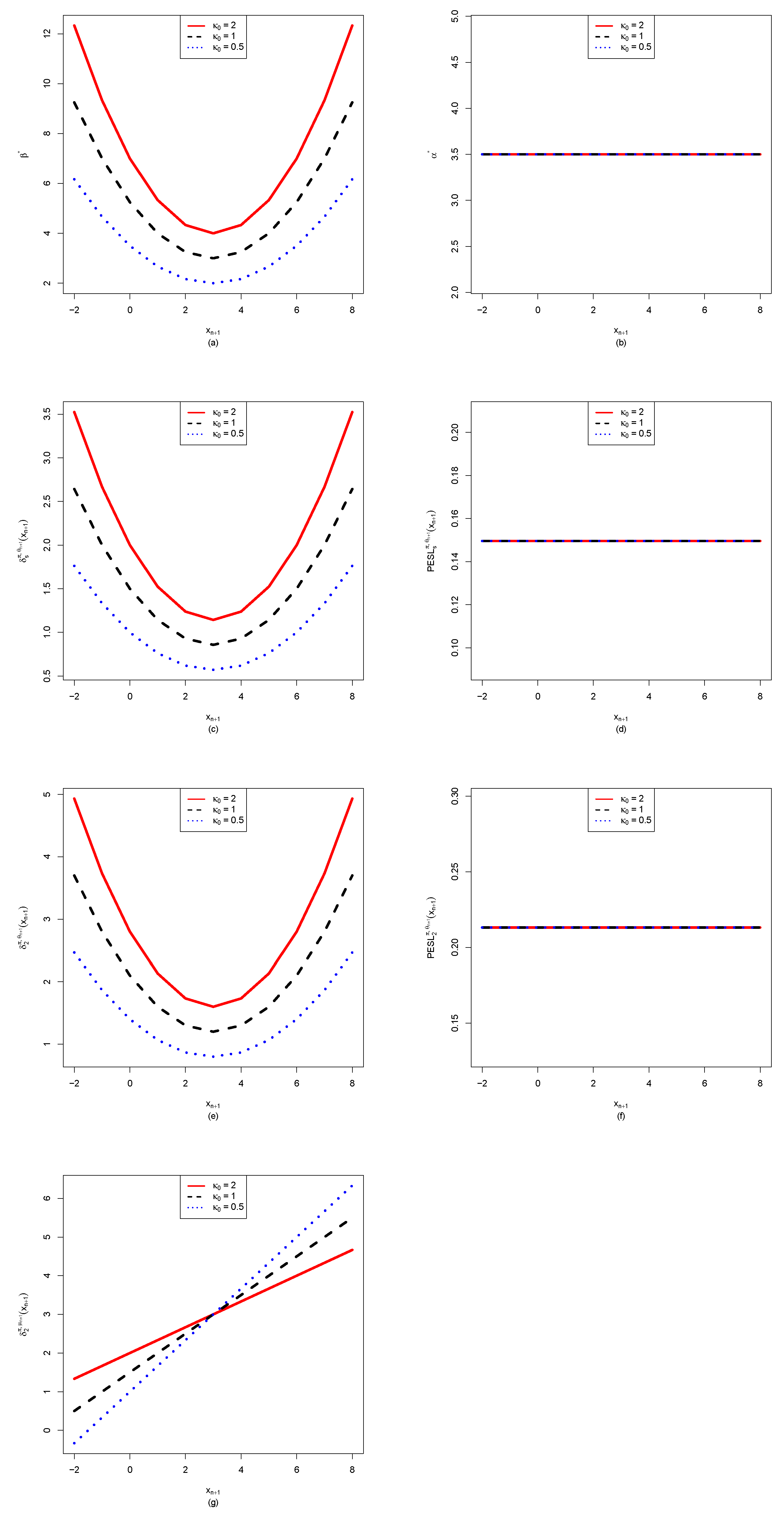
Figure 3.
The histogram of and the density estimation curve of .
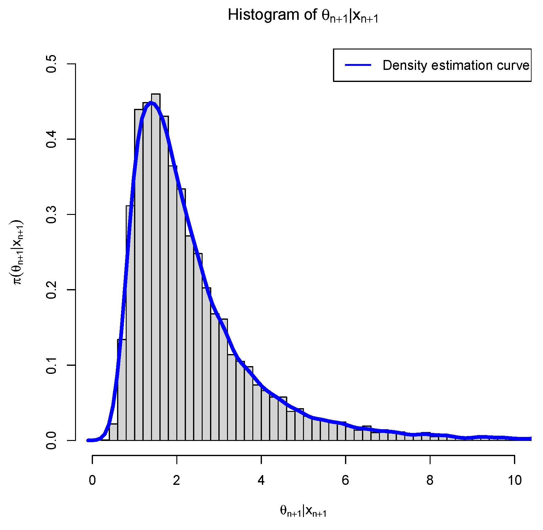
Figure 4.
The Bayes estimators and the PESLs as functions of . (a) Bayes estimators vs . (b) PESLs vs .
Figure 4.
The Bayes estimators and the PESLs as functions of . (a) Bayes estimators vs . (b) PESLs vs .
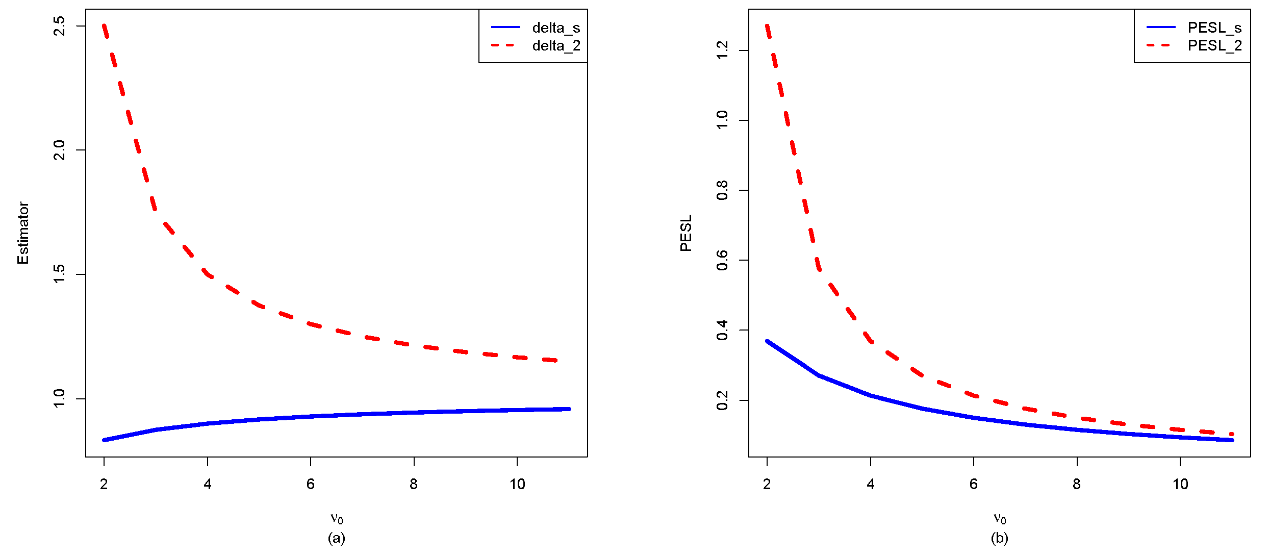
Figure 5.
The Bayes estimators and the PESLs as functions of , , , and . (a), (c), (e), (g) Bayes estimators vs , , , and . (b), (d), (f), (h) PESLs vs , , , and .
Figure 5.
The Bayes estimators and the PESLs as functions of , , , and . (a), (c), (e), (g) Bayes estimators vs , , , and . (b), (d), (f), (h) PESLs vs , , , and .
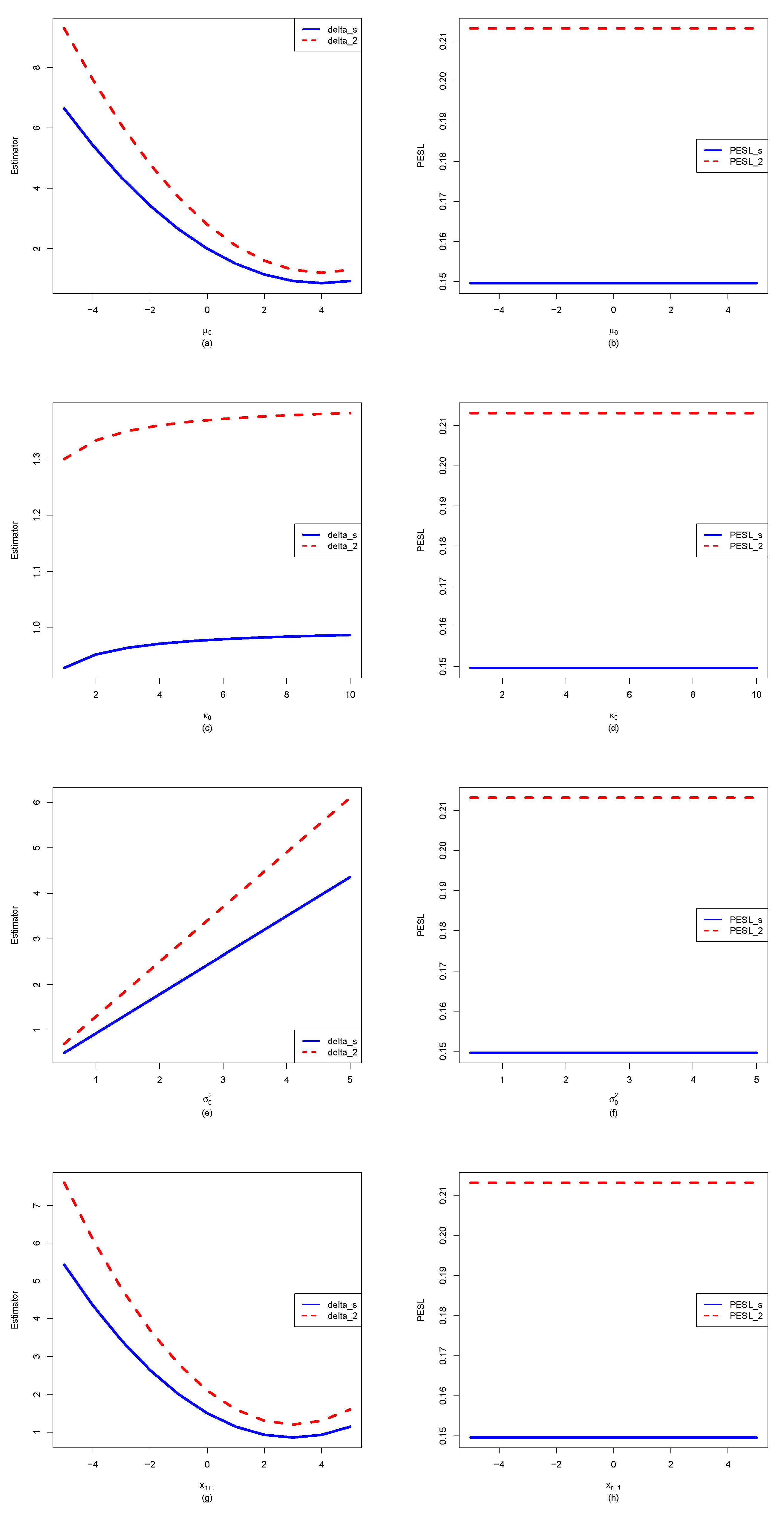
Figure 6.
The domain for is for all the plots. a is for and b is for in the axes of all the plots. The red surface is for and the blue surface is for in the upper two plots. (a) The estimators as functions of and . for all on D. (b) The PESLs as functions of and . for all on D. (c) The surface of which is positive for all on D. (d) The surface of which is also positive for all on D.
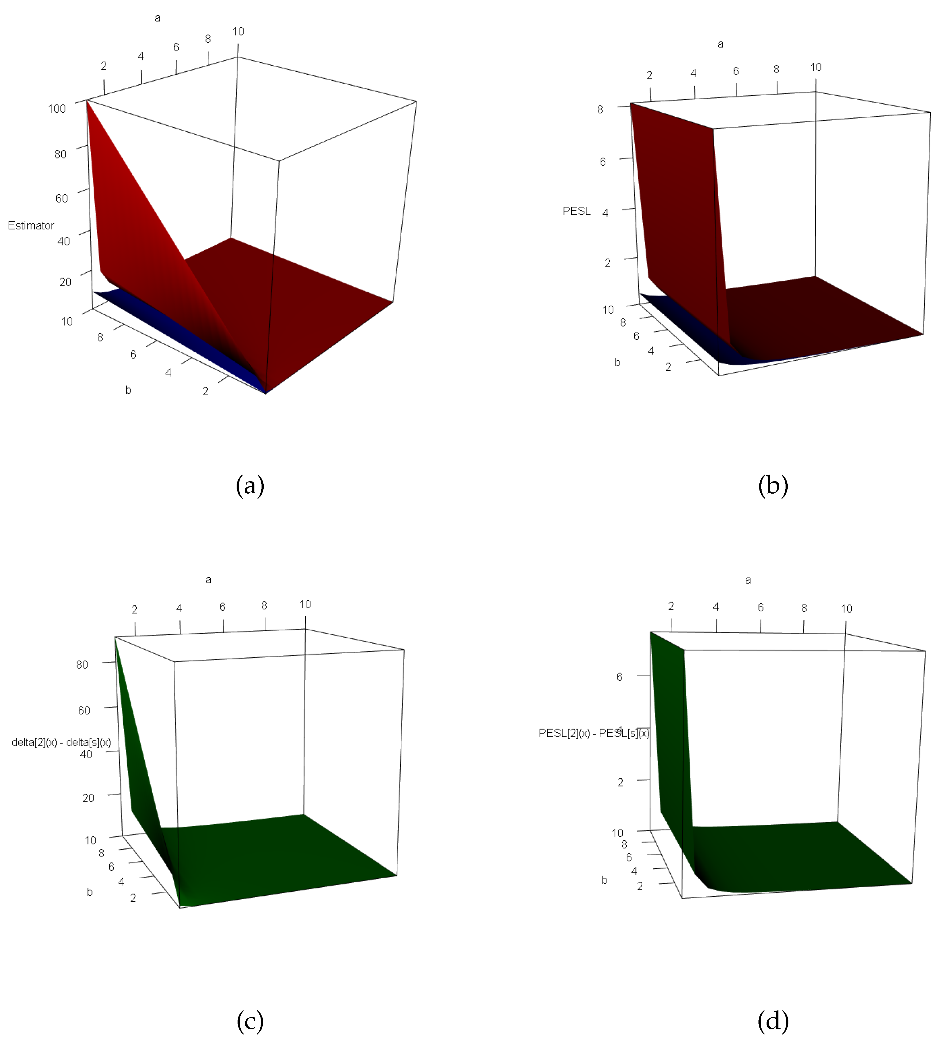
Figure 7.
The boxplots of the D values and the p-values for the three methods. (a) D values. (b) p-values.
Figure 7.
The boxplots of the D values and the p-values for the three methods. (a) D values. (b) p-values.
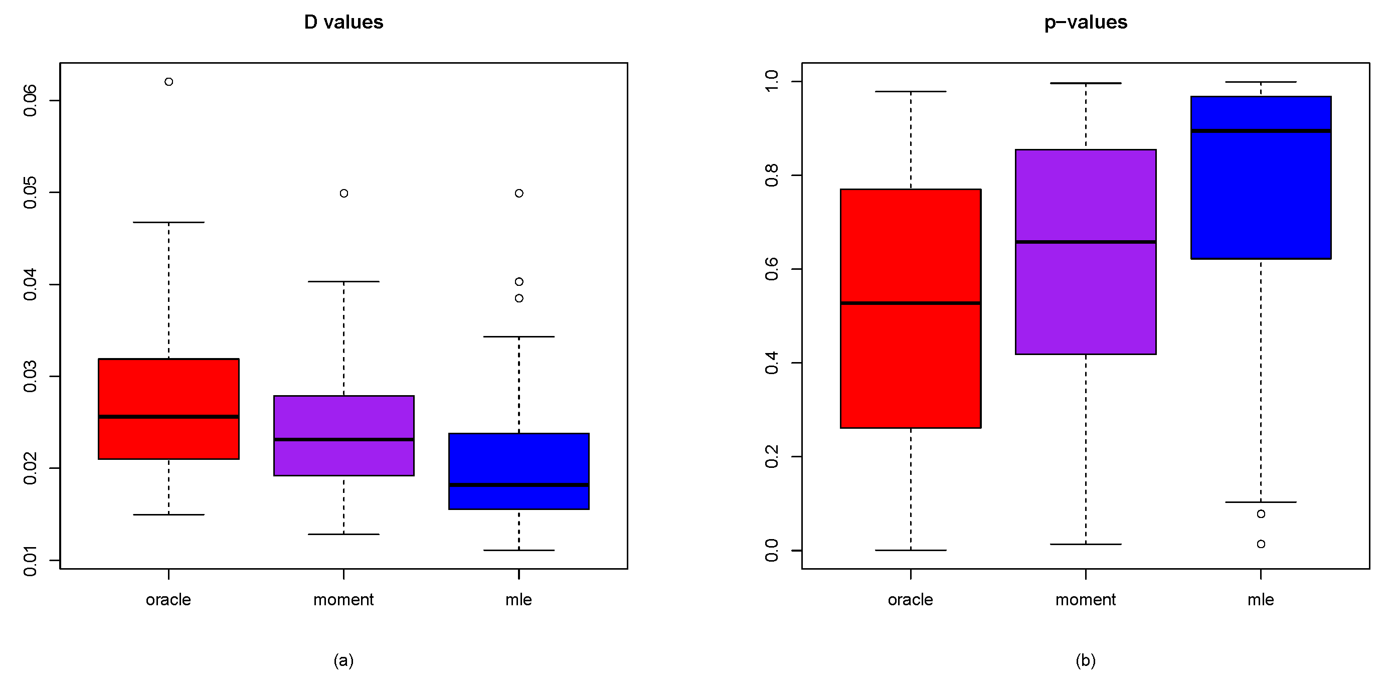
Figure 8.
The marginal densities for varied , holding , , and fixed.
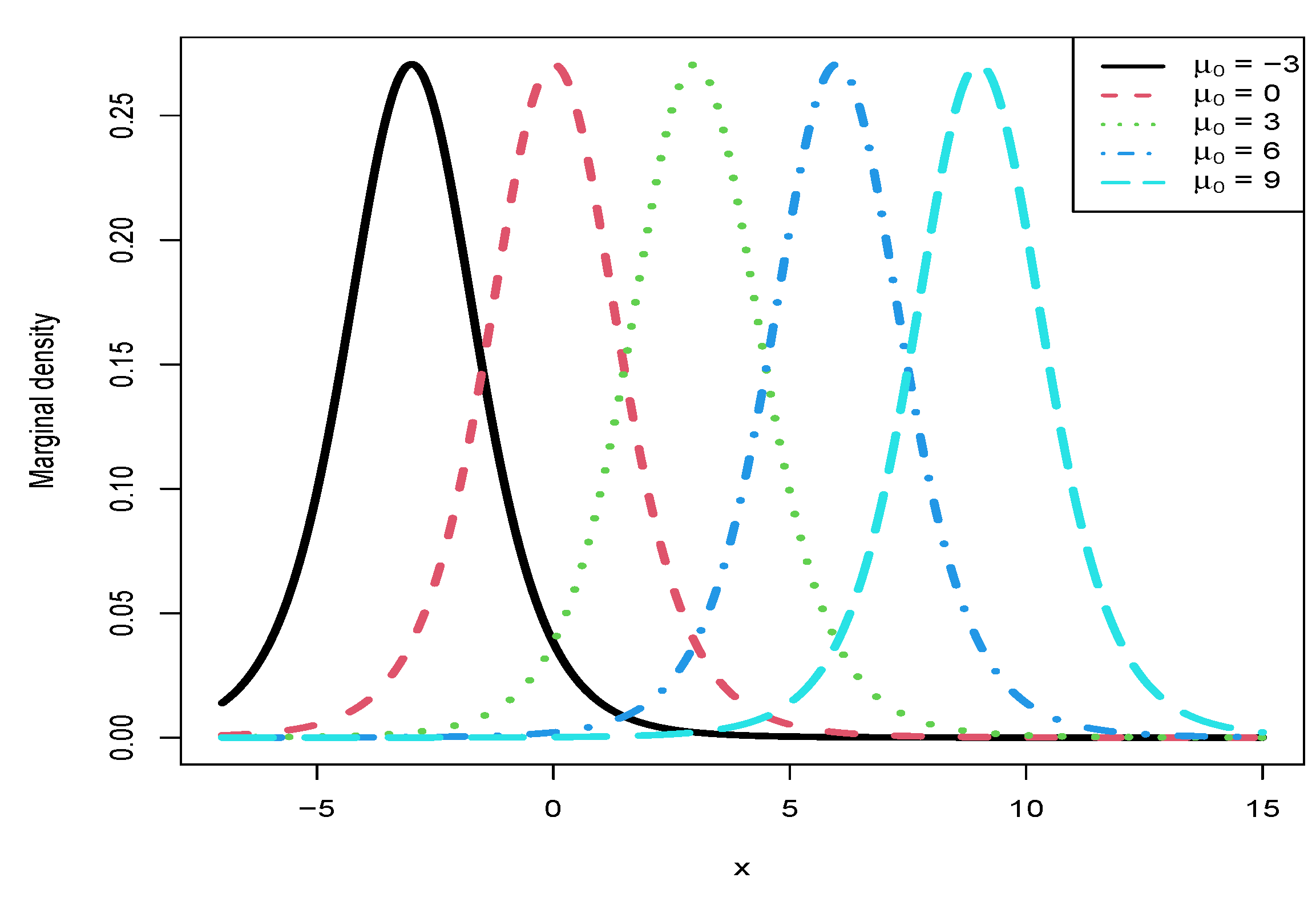
Figure 9.
The marginal densities for varied , holding , , and fixed.

Figure 10.
The marginal densities for varied , holding , , and fixed.
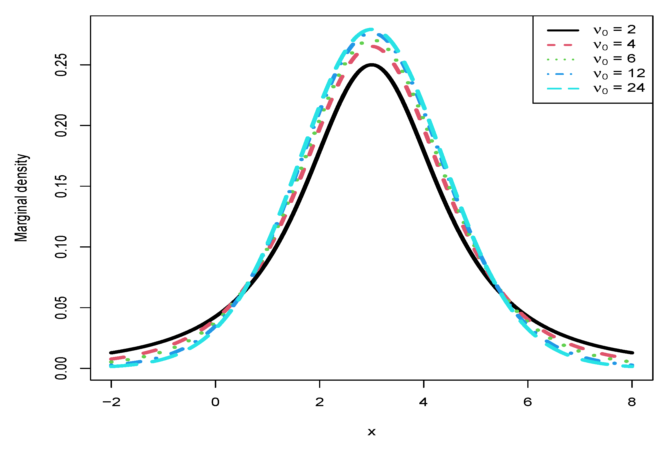
Figure 11.
The marginal densities for varied , holding , , and fixed.
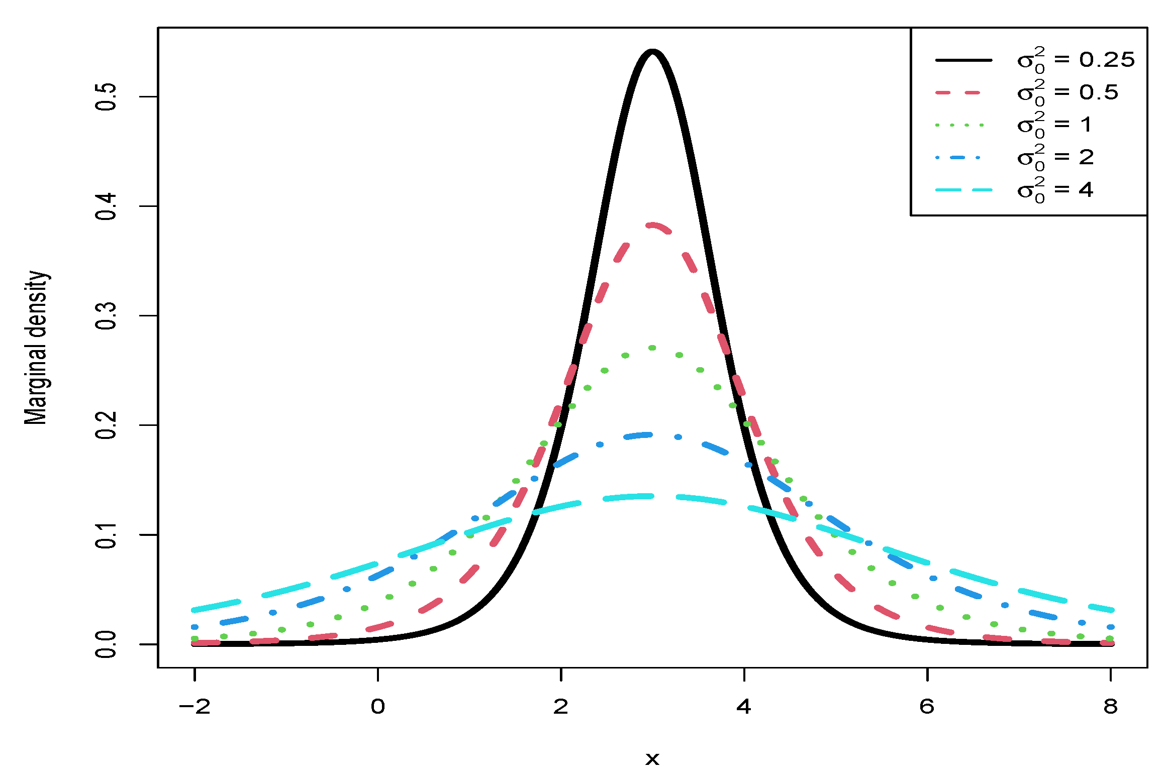
Figure 12.
The histogram of the sample and its density estimation curve.
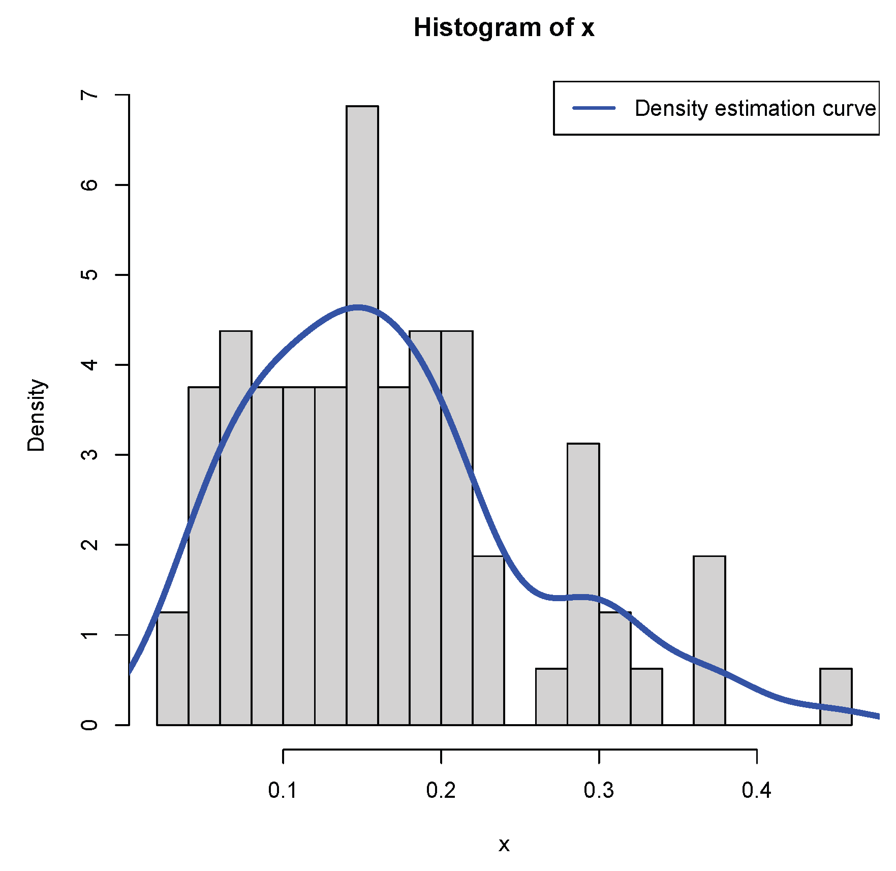

Table 1.
The moment estimators and the MLEs of the hyperparameters for the samples , , and .
| Moment estimators | MLEs | |
Table 2.
The frequencies of the moment estimators and the MLEs of the hyperparameters as n varies for , , and .
Table 2.
The frequencies of the moment estimators and the MLEs of the hyperparameters as n varies for , , and .
| Moment estimators | MLEs | ||||||
| n | |||||||
| 1e4 | |||||||
| 2e4 | |||||||
| 4e4 | |||||||
| 8e4 | |||||||
| 16e4 | |||||||
| 1e4 | |||||||
| 2e4 | |||||||
| 4e4 | |||||||
| 8e4 | |||||||
| 16e4 | |||||||
| 1e4 | |||||||
| 2e4 | |||||||
| 4e4 | |||||||
| 8e4 | |||||||
| 16e4 | |||||||
Table 3.
The numerical values of the Bayes estimators and the PESLs in Figure 4: changes.
Table 3.
The numerical values of the Bayes estimators and the PESLs in Figure 4: changes.
| 2 | 3 | 4 | 5 | 6 | 7 | 8 | 9 | 10 | 11 | |
Table 4.
The numerical values of the Bayes estimators and the PESLs in Figure 5: changes.
Table 4.
The numerical values of the Bayes estimators and the PESLs in Figure 5: changes.
| 0 | 1 | 2 | 3 | 4 | 5 | ||||||
Table 5.
The numerical values of the Bayes estimators and the PESLs in Figure 5: changes.
Table 5.
The numerical values of the Bayes estimators and the PESLs in Figure 5: changes.
| 1 | 2 | 3 | 4 | 5 | 6 | 7 | 8 | 9 | 10 | |
Table 6.
The numerical values of the Bayes estimators and the PESLs in Figure 5: changes.
Table 6.
The numerical values of the Bayes estimators and the PESLs in Figure 5: changes.
| 1 | 2 | 3 | 4 | 5 | ||||||
Table 7.
The numerical values of the Bayes estimators and the PESLs in Figure 5: changes.
Table 7.
The numerical values of the Bayes estimators and the PESLs in Figure 5: changes.
| 0 | 1 | 2 | 3 | 4 | 5 | ||||||
Table 8.
The results of the KS test goodness-of-fit of the model (2) to the simulated data.
Table 8.
The results of the KS test goodness-of-fit of the model (2) to the simulated data.
Table 9.
The estimators of the hyperparameters, the goodness-of-fit of the model, the empirical Bayes estimators of the variance parameter of the normal distribution and the PESLs, and the mean and variance of the real data by the moment method and the MLE method.
Table 9.
The estimators of the hyperparameters, the goodness-of-fit of the model, the empirical Bayes estimators of the variance parameter of the normal distribution and the PESLs, and the mean and variance of the real data by the moment method and the MLE method.
| Moment method | MLE method | ||
| Estimators of | |||
| the hyperparameters | |||
| Goodness-of-fit | D | ||
| of the model | p-value | ||
| Empirical Bayes estimators | |||
| and PESLs | |||
| Mean and variance of | |||
| the poverty level data |
Disclaimer/Publisher’s Note: The statements, opinions and data contained in all publications are solely those of the individual author(s) and contributor(s) and not of MDPI and/or the editor(s). MDPI and/or the editor(s) disclaim responsibility for any injury to people or property resulting from any ideas, methods, instructions or products referred to in the content. |
© 2025 by the author. Licensee MDPI, Basel, Switzerland. This article is an open access article distributed under the terms and conditions of the Creative Commons Attribution (CC BY) license (http://creativecommons.org/licenses/by/4.0/).
Copyright: This open access article is published under a Creative Commons CC BY 4.0 license, which permit the free download, distribution, and reuse, provided that the author and preprint are cited in any reuse.


